Determination of the carrier diffusion length in GaN from cathodoluminescence maps around threading dislocations: fallacies and opportunities
Vladimir M. Kaganer, Jonas L\"ahnemann, Carsten Pf\"uller, Karl K., Sabelfeld, Anastasya E. Kireeva, Oliver Brandt

TL;DR
This study combines theoretical and experimental approaches to analyze exciton behavior around threading dislocations in GaN, revealing that cathodoluminescence energy contrast, not intensity, can be used to determine exciton diffusion length.
Contribution
It demonstrates that cathodoluminescence intensity contrast is not suitable for measuring diffusion length, but energy contrast provides a reliable method for its determination in GaN.
Findings
Cathodoluminescence intensity contrast is weakly affected by exciton diffusion.
Energy contrast in cathodoluminescence maps depends on exciton diffusion length.
Dark spot size around dislocations does not indicate exciton diffusion length.
Abstract
We investigate, both theoretically and experimentally, the drift, diffusion, and recombination of excitons in the strain field of an edge threading dislocation intersecting the GaN{0001} surface. We calculate and measure hyperspectral cathodoluminescence maps around the dislocation outcrop for temperatures between 10 to 200 K. Contrary to common belief, the cathodoluminescence intensity contrast is only weakly affected by exciton diffusion, but is caused primarily by exciton dissociation in the piezoelectric field at the dislocation outcrop. Hence, the extension of the dark spots around dislocations in the luminescence maps cannot be used to determine the exciton diffusion length. However, the cathodoluminescence energy contrast, reflecting the local bandgap variation in the dislocation strain field, does sensitively depend on the exciton diffusion length and hence enables its…
Click any figure to enlarge with its caption.
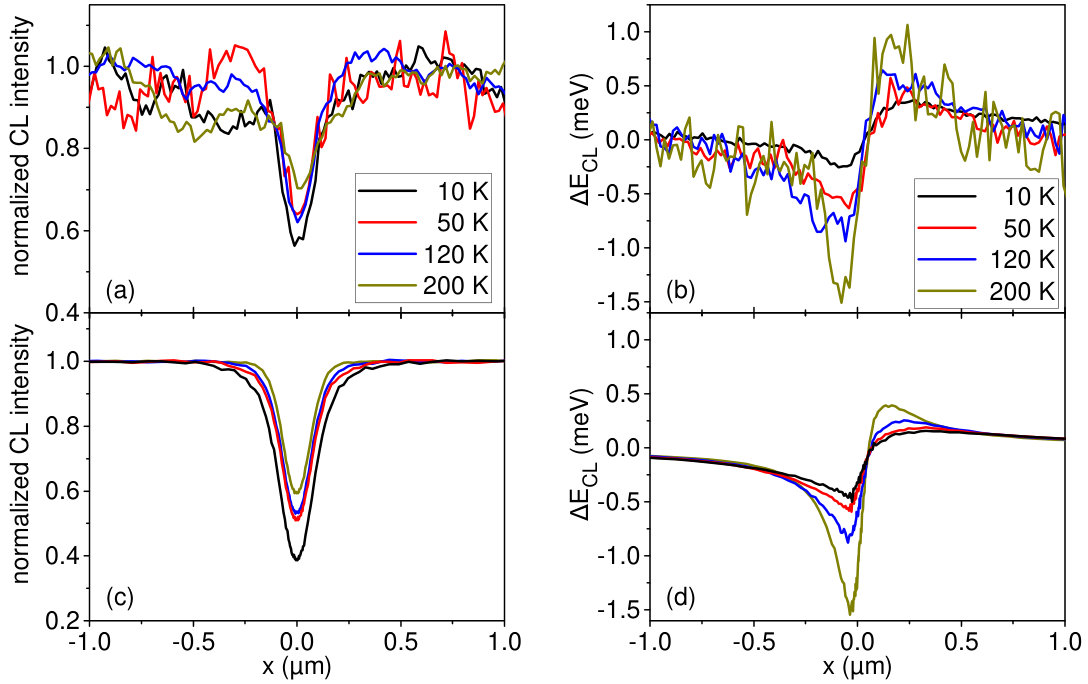 Figure 1
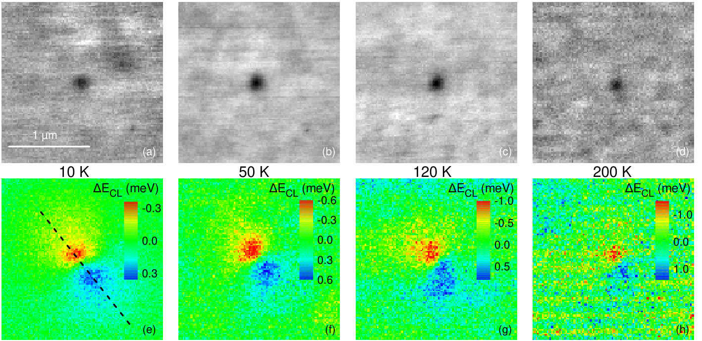 Figure 2
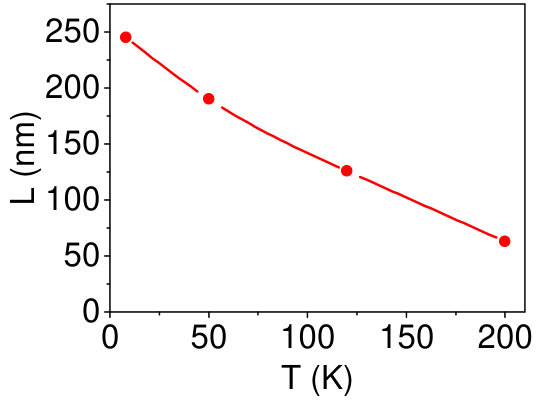 Figure 3
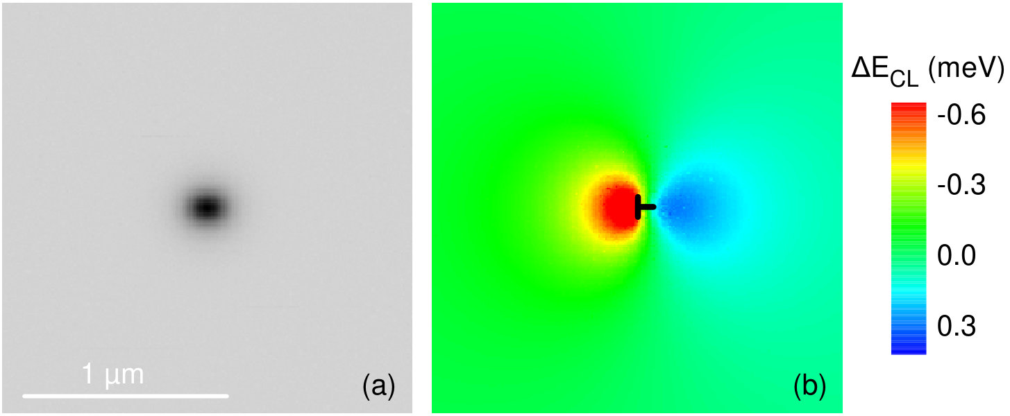 Figure 4
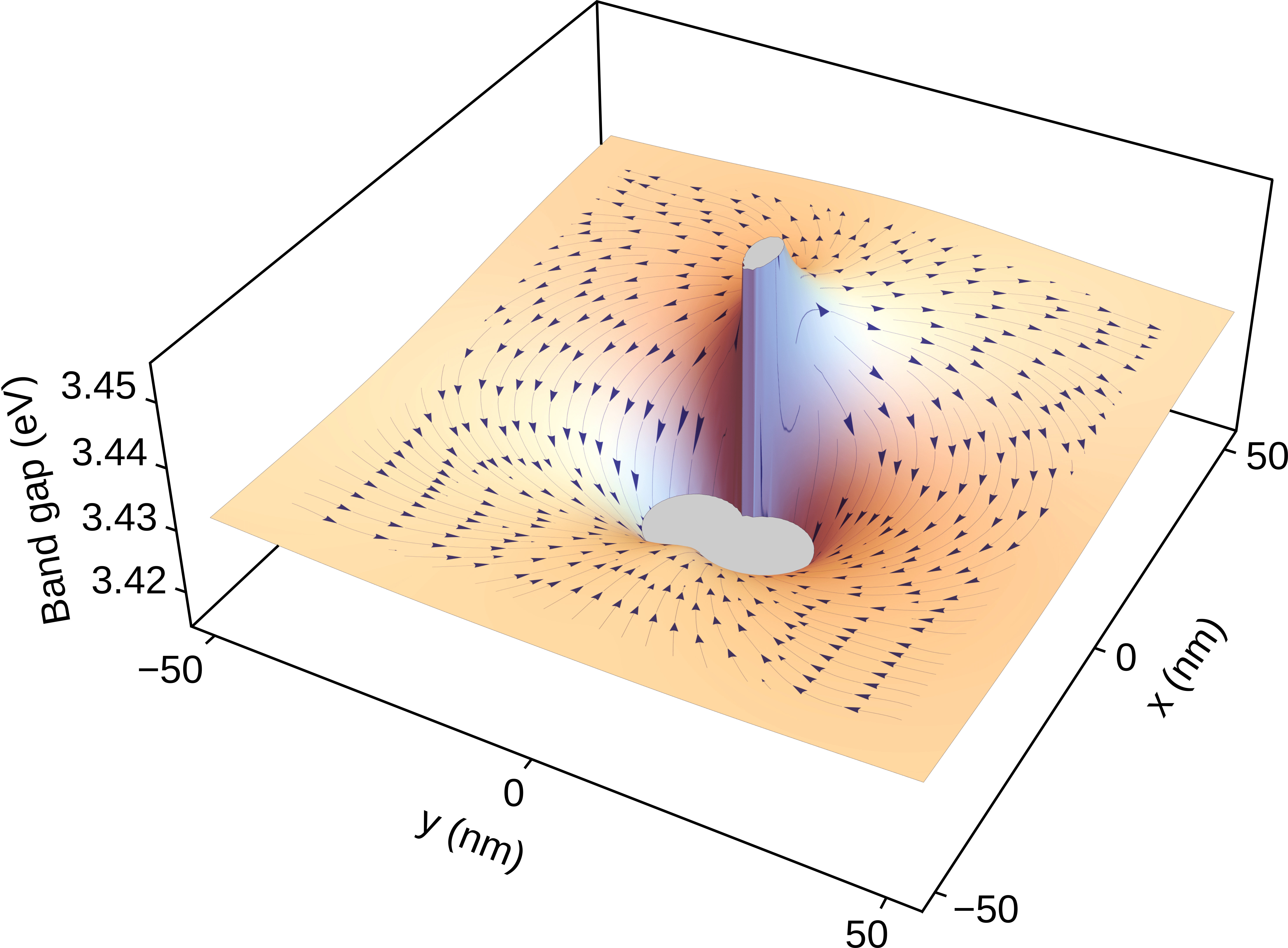 Figure 5
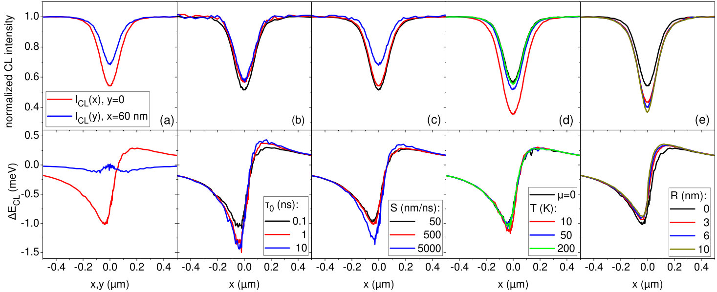 Figure 6
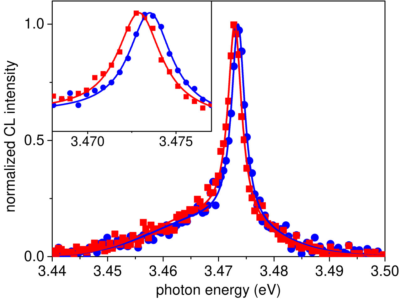 Figure 7
Peer Reviews
No public reviews on file for this paper yet. If you reviewed it on a platform where reviews are public (OpenReview, ICLR, NeurIPS, ICML), you can paste yours below so the community can read it here.
Videos
No videos yet. Explain this paper in a talk, walkthrough, or lecture? Add one.
Determination of the carrier diffusion length in GaN from cathodoluminescence maps around threading dislocations: fallacies and opportunities
Vladimir M. Kaganer
Paul-Drude-Institut für Festkörperelektronik, Leibniz-Institut im Forschungsverbund Berlin e. V., Hausvogteiplatz 5–7, 10117 Berlin, Germany
Jonas Lähnemann
Paul-Drude-Institut für Festkörperelektronik, Leibniz-Institut im Forschungsverbund Berlin e. V., Hausvogteiplatz 5–7, 10117 Berlin, Germany
Carsten Pfüller
Paul-Drude-Institut für Festkörperelektronik, Leibniz-Institut im Forschungsverbund Berlin e. V., Hausvogteiplatz 5–7, 10117 Berlin, Germany
Karl K. Sabelfeld
Institute of Computational Mathematics and Mathematical Geophysics, Russian Academy of Sciences, Lavrentiev Prosp. 6, 630090 Novosibirsk, Russia
Anastasya E. Kireeva
Institute of Computational Mathematics and Mathematical Geophysics, Russian Academy of Sciences, Lavrentiev Prosp. 6, 630090 Novosibirsk, Russia
Oliver Brandt
Paul-Drude-Institut für Festkörperelektronik, Leibniz-Institut im Forschungsverbund Berlin e. V., Hausvogteiplatz 5–7, 10117 Berlin, Germany
Paul-Drude-Institut für Festkörperelektronik, Leibniz-Institut im Forschungsverbund Berlin e. V., Hausvogteiplatz 5–7, 10117 Berlin, Germany
Paul-Drude-Institut für Festkörperelektronik, Leibniz-Institut im Forschungsverbund Berlin e. V., Hausvogteiplatz 5–7, 10117 Berlin, Germany
Paul-Drude-Institut für Festkörperelektronik, Leibniz-Institut im Forschungsverbund Berlin e. V., Hausvogteiplatz 5–7, 10117 Berlin, Germany
Institute of Computational Mathematics and Mathematical Geophysics, Russian Academy of Sciences, Lavrentiev Prosp. 6, 630090 Novosibirsk, Russia
Institute of Computational Mathematics and Mathematical Geophysics, Russian Academy of Sciences, Lavrentiev Prosp. 6, 630090 Novosibirsk, Russia
Paul-Drude-Institut für Festkörperelektronik, Leibniz-Institut im Forschungsverbund Berlin e. V., Hausvogteiplatz 5–7, 10117 Berlin, Germany
Abstract
We investigate, both theoretically and experimentally, the drift, diffusion, and recombination of excitons in the strain field of an edge threading dislocation intersecting the GaN{0001} surface. We calculate and measure hyperspectral cathodoluminescence maps around the dislocation outcrop for temperatures between 10 to 200 K. Contrary to common belief, the cathodoluminescence intensity contrast is only weakly affected by exciton diffusion, but is caused primarily by exciton dissociation in the piezoelectric field at the dislocation outcrop. Hence, the extension of the dark spots around dislocations in the luminescence maps cannot be used to determine the exciton diffusion length. However, the cathodoluminescence energy contrast, reflecting the local bandgap variation in the dislocation strain field, does sensitively depend on the exciton diffusion length and hence enables its experimental determination.
I Introduction
The minority carrier, ambipolar, or exciton diffusion length is the quantity that governs all scenarios where electrons and holes or excitons diffuse and recombine, and is as such one of the crucial parameters that controls the behavior of semiconductor devices. A popular method to experimentally determine the diffusion length relies on the perception that threading dislocations in semiconductors are line defects that act as nonradiative sinks for minority charge carriers. The zone of reduced luminescence intensity around the dislocation is thus related to the carrier or exciton diffusion length [1; 2; 3; 4; 5; 6; 7; 8].
This method has been frequently employed to determine the exciton diffusion length in GaN(0001) films, for which threading dislocations are visible as dark spots in cathodoluminescence (CL) or electron-beam induced current (EBIC) maps [9; 10; 11; 12; 13; 14; 15; 16]. In the majority of previous experimental work, the diffusion length was extracted from the available data in a simple phenomenological fashion that had no sound physical foundation. We have recently derived a rigorous solution for the intensity contrast around threading dislocations in GaN{0001} considering fully three-dimensional generation, diffusion and recombination of excitons in the presence of a surface and a dislocation both possessing finite recombination strengths [17]. Our study has shown that the phenomenological expression adopted in previous work does not represent a sensible approximation of this intensity profile, and in fact leads to a gross underestimation of the diffusion length.
In a subsequent work, we have shown that the relaxation of strain at the outcrop of edge threading dislocations in GaN{0001} gives rise to a piezoelectric field with a strength sufficient to dissociate free excitons and to spatially separate electrons and holes at distances over 100 nm from the dislocation line [18]. The spatial separation inhibits radiative recombination of the electron-hole pairs, and edge threading dislocations hence give rise to dark spots in CL maps very similar to those observed experimentally even in the absence of exciton diffusion. This result raises the question to what extent the intensity contrast is actually still affected by exciton diffusion, if at all.
Moreover, the strain field around a dislocation gives rise to a second effect that so far has not been taken into consideration in the analysis of the intensity contrast. The inhomogeneous strain field of a dislocation [19; 20] induces a change of the band gap around the dislocation via the deformation potential mechanism [21; 22; 23; 24]. The quasi-electric field of the band gap gradient around the dislocation leads in turn to a drift of excitons in the strain field. Consequently, the flux of excitons toward the dislocation, and thus the luminous intensity due to their nonradiative annihilation at the dislocation, is affected not only by diffusion but also by drift in the dislocation strain field. The magnitudes of the drift and diffusion fluxes are connected by the Einstein relation, but their driving forces are distinctly different, and the directions of the fluxes may coincide or oppose each other. In other words, exciton drift may enhance or counteract the effects of exciton diffusion. In general, drift tends to concentrate, whereas diffusion dissolves.
In the present work, we extend our previous theoretical framework [17] and explicitly consider, in addition to exciton diffusion, the effects of the three-dimensional strain distribution associated to an edge threading dislocation at the GaN{0001} surface, i. e., exciton drift in the strain field and exciton dissociation in the piezoelectric field induced by the changes in strain. We solve this complex three-dimensional problem by an advanced Monte Carlo scheme [25; 26]. For comparison with the theoretical predictions, we record hyperspectral CL maps around the outcrop of a threading dislocation of a free-standing GaN(0001) film. To facilitate the clear distinction of the effects of exciton drift and diffusion, these maps are recorded for various temperatures ranging from 10 to 200 K. Our measurements show that the CL intensity profiles do not notably depend on temperature, despite the fact that the diffusion length is known to significantly decrease with increasing temperature. In contrast, the CL energy profile is observed to depend strongly on temperature. These findings are reproduced by our simulations. Our results show that the common understanding of a diffusion-controlled intensity contrast around threading dislocations in GaN{0001} is a misconception. The mechanism dominating the intensity contrast is the piezoelectric field around the dislocation outcrop, and exciton diffusion changes this contrast only marginally. However, the energy contrast turns out to be highly sensitive to the diffusion length, which we thus propose as a new experimental observable for the actual determination of the carrier diffusion length in GaN.
II Methods
The CL experiments were performed on the same free-standing GaN(0001) layer grown by hydride vapor phase epitaxy as used in our previous investigation [17]. The density of threading dislocations reaching the surface of this layer amounts to cm*-2*. CL spectroscopy was carried out using a Zeiss Ultra55 field-emission scanning electron microscope equipped with a Gatan MonoCL4 system and a He-cooling stage. The acceleration voltage was set to 3 kV, and the probe current of the electron beam to 1.1 nA, with the aim to minimize the generation volume of excitons as much as possible. The electron beam diameter was 5 nm, significantly smaller than the step size of 20 nm chosen for recording CL maps. Hyperspectral maps were acquired in the vicinity of isolated threading dislocations for temperatures between 10 and 200 K, using a parabolic mirror to collect the emitted light, a spectrometer for dispersing it with the spectral resolution set to 3 meV, and a charge-coupled device as the detector. Analysis of the CL data was performed using the Python package HyperSpy [27].
The calculations of the CL intensity and energy around an edge threading dislocation were performed using an advanced Monte Carlo scheme developed previously for the solution of the pure diffusion problem [25], but extended to include exciton drift in the strain field of the dislocation [26], and exciton dissociation in the associated electric field [18]. The algorithm is described in detail in the Supplementary Material. The material constants entering the model (particularly the elastic moduli and the piezoelectric coefficients and of GaN) were taken the same as in [18]. The value of the shear piezoelectric coefficient strongly influences the CL intensity profiles [18], and was here assumed to be . The surface recombination velocity is taken to be nm/ns [28]. The diffusion coefficient is assumed to be nm2/ns independent of temperature since its temperature dependence is comparatively weak [29]. Only one quantity entering the model, namely, the exciton lifetime far from the dislocation, is treated as adjustable parameter.
III The drift-diffusion-recombination problem
We consider the generation of electron-hole pairs by an electron beam incident on the surface of a GaN{0001} layer. In a CL or an EBIC experiment, a tightly focused electron beam scans the sample and generates electron-hole pairs. For the electron beam position , the initial density of the electron-hole pairs generated by the electron beam at a point in the sample is described by a three-dimensional generation function . At low temperatures, these electron-hole pairs rapidly bind to form excitons. At higher temperatures, thermal dissociation results in the coexistence of excitons and free carriers, with the ratio of their concentrations being controlled by the Saha equation [30]. Because of the exciton binding energy of 26 meV in GaN, and the comparatively high excitation density in CL, the fraction of excitons remains large in the entire temperature range of our experimental investigations. For simplicity, we therefore refer exclusively to excitons in the following. It is important to note, however, that the formalism we develop applies equally well for minority carrier or ambipolar diffusion of electrons and holes*, *the only difference being the value of the diffusion coefficient. The aim of this section is to formulate the problem of exciton diffusion, drift, and recombination in the half-space containing a dislocation line normal to the surface, with nonradiative annihilation of the excitons at the free surface and in the vicinity of the dislocation line.
Diffusion of excitons gives rise to the diffusional flux , where is the diffusion coefficient and is the three-dimensional distribution of the exciton density for a given position of the exciting electron beam. The spatial variation of the band gap due to the inhomogeneous strain of the dislocation gives rise to the exciton drift velocity , where is the exciton mobility, and to the drift flux . The diffusion coefficient and the mobility are related by the Einstein relation , where is the Boltzmann constant and is the temperature.
The band gap of a strained semiconductor generally depends on all components of the strain tensor [21]. However, the effect of shear strain is notably smaller than that of normal strain. Since screw (-type) threading dislocations induce only shear strain, they have little effect on the band gap. Consequently, we focus in this paper on the effect of the edge component of an edge (-type) or mixed (-type) threading dislocation. Figure 1 shows the variation of the band gap of GaN in the vicinity of an a-type edge dislocation located at together with the respective drift velocity , calculated in the framework of a Bir-Pikus approach [22] taking into account both normal and shear strain components. The shear strain gives rise to an asymmetry between the regions of increased and decreased bandgap. The surface relaxation strain is not included in the calculation here, so that the band gap and the drift velocity shown in Fig. 1 are reached at the distances from the surface large compared to the respective lateral distance. Hence, the whole map corresponds to depths larger than 50 nm (while the central part is not affected by the surface relaxation strain also at smaller depths). The band gap increases in the region of compressive strain at one side and decreases in the region of tensile strain at the other side of the dislocation line. Due to the drift, excitons are hence repelled at one side of the dislocation and attracted at the other side.
The total flux of excitons is the sum of the diffusion and the drift fluxes,
[TABLE]
and the steady-state continuity equation reads
[TABLE]
In this equation, is the exciton lifetime. It contains contributions from the radiative lifetime , the nonradiative lifetime in the crystal far from dislocations, and the position-dependent lifetime describing the rate of the exciton dissociation in the piezoelectric field near the dislocation outcrop [18]. Combining the rates of the two nonradiative processes in one term, , we can represent the total recombination rate as
[TABLE]
The drift-diffusion equation can thus be written as
[TABLE]
Nonradiative exciton annihilation at the planar surface is described by the boundary condition
[TABLE]
where is the surface of the half-infinite crystal, the outward surface normal vector, and the surface recombination velocity. A similar boundary condition, with an analogous recombination velocity, has been written at the dislocation line represented by a thin cylinder [17].
Let us integrate Eq. (2) over the sample volume. In the first term of the equation, we proceed from a volume to a surface integral, yielding the rate of exciton annihilation at the surface ,
[TABLE]
This quantity can be directly measured in EBIC experiments. In the second term of Eq. (2), we separate the radiative and the nonradiative contributions, which gives
[TABLE]
The right hand side of this equation is the total number of excitons generated per unit time. The terms in the left hand side are the flux to the surface and the number of excitons recombining per unit time radiatively and nonradiatively, respectively. The total photon flux
[TABLE]
is the quantity measured in a CL experiment, and our primary aim is its calculation.
An exciton radiatively recombining at some point in the sample produces a photon whose energy is equal to , where is the local bandgap and is the exciton binding energy. Depending on the position of the electron beam with respect to the dislocation, the photons are predominantly generated in the regions of compression or tension in the dislocation strain field, giving rise to blue and red shifts of the exciton line, respectively [31; 32]. The exciton line position is given by averaging the photon energy over the distribution of excitons recombining radiatively. This conditional expectation is
[TABLE]
and it is calculated in the present work together with the CL intensity distribution, and compared with the experimental results.
The drift-diffusion problem could in principle be solved by a direct Monte Carlo modeling of random walks on a grid performed by particles generated from the source, with a finite lifetime and a partial annihilation at the boundaries. Such modeling was performed, for pure diffusion with constant lifetime and neglecting drift, in Refs. [33; 34; 35]. However, a direct modeling of a three-dimensional random walk is extremely time-consuming, since the particle makes many random steps before it annihilates in the bulk or meets a boundary.
An efficient Monte Carlo algorithm developed for the diffusion problem [25] and generalized recently to the drift-diffusion problem [26] replaces the random walk inside a sphere by a single, appropriately modeled, step from the center of the sphere to its surface. The sphere radius can be taken equal to the distance to the nearest surface. The survival probability for the particle to reach the sphere, depending on its finite lifetime, is explicitly calculated. If the particle survives, it jumps to a random point on the sphere, and the next sphere is generated with its radius given by the distance from the new position to the nearest surface. It has been shown that the sequence of spheres converges to the boundary. The mean number of steps required to reach a distance from the boundary is proportional to , so that even for a very small value of the mean number of steps in this process is quite small. The behavior of the particle after it hits the -vicinity of the surface is described separately, in accordance with the given boundary conditions. A detailed account of the Monte Carlo algorithm for the solution of the drift-diffusion problem can be found in the Supplementary Material.
IV Results
For recording hyperspectral maps around the outcrop of threading dislocations, the electron beam was raster-scanned across the sample surface of µm2 containing the dislocation of interest with a sampling step size, i. e., a spatial pixel, of 20 nm. At every step, a full CL spectrum was recorded in the energy range from 3.2 to 3.8 eV, covering all free and bound exciton transitions for our free-standing GaN layer [36]. We have investigated a significant number () of dislocations for this sample, and the results shown below are representative for all dislocations and vary within %.
Figure 2 shows two exemplary CL spectra taken from such a map recorded around a selected threading dislocation at 10 K. The spectra correspond to the points in the maps exhibiting the maximum blue and red shift close to the outcrop of the threading dislocation. Each spectrum was fit by the sum of a Lorentzian and a Gaussian accounting for the dominant high-energy line stemming from donor-bound exciton recombination [37], and the low-energy shoulder originating from acceptor-bound excitons as well as from the two electron satellites of the donor-bound exciton [38], respectively, as shown in Fig. 2 (for maps acquired at 50, 120, and 200 K, no bound exciton transition is observed and the fits to the free A exciton line [39; 40] were done with a single Lorentzian).
The sharp lines in Fig. 2 are resolution limited, with the full width at half maximum (FWHM) of 3 meV. The accuracy of the spectral positions of the lines is governed by statistical fluctuations of the CL intensity and amounts to 0.04 meV, as obtained from the fits shown in Fig. 2. The lines broaden with increasing temperature and reach a FWHM of 25 meV at 200 K. The accuracy than reduces to 0.4 meV, because of larger statistical fluctuations of the intensity. Since the lineshifts in the vicinity of the dislocation also increase with temperature, as it is demonstrated below, the accuracy is still sufficient to systematically study both CL intensity and line positions. However, the measurements at temperatures above 200 K are too noisy for a reliable analysis.
For each temperature, the fits yield maps of the spectrally integrated intensity of the dominant exciton transition and its spectral position, as shown in Figs. 3(a–d) and Figs. 3(e–h), respectively. The maps clearly reveal the reduced CL intensity and the shift of the transition energy at the outcrop of the threading dislocation. Note that the maps were taken from one and the same dislocation for all temperatures.
The red and the blue lobes in the maps in Figs. 3(e–h) correspond to regions of tensile and compressive strain around the dislocation, respectively, and hence demonstrate that this dislocation is of either or type. Since the screw component induces only shear strain with a minor effect on the band gap, we cannot distinguish pure edge and mixed dislocations. The line shift increases with temperature and reaches 2.5 meV at 200 K. At the same time, the statistical error of the fits increases due to the thermal quenching of the emission intensity and the resulting increasing noise in the spectra, thus leading to a higher noise level also in the maps.
Figures 4(a,b) show simulated maps of the spectrally integrated CL intensity and CL spectral line positions around an edge threading dislocation, respectively. Evidently, the maps are close to the experimentally recorded maps shown in Fig. 3. In the CL intensity map, the dislocation outcrop is associated with a dark spot with FWHM of about 200 nm. The intensity distribution appears to be almost isotropic, i. e., the anisotropy of the piezoelectric field around the dislocation [18] is effectively smoothed out by exciton diffusion. The change in the CL line position is seen at distances up to 1 µm from the dislocation. The cut of an extra plane at the dislocation line indicated in Fig. 4(b) shows the dislocation position at . One can see that a vertical line separating the blue and red lobes does not pass through the dislocation position but is shifted with respect to it. Lattice compression in the right part gives rise to a blue shift, while lattice expansion in the left part induces a red shift.
For a quantitative analysis, Figs. 5(a,b) show the integrated intensity and the spectral position of the exciton transition obtained by line scans across the strain dipole of the dislocation [dashed line in Fig. 3(e)] in Figs. 3(a–h). Figure 5(a) clearly shows that the width of the CL intensity curves does not notably depend on temperature, although the diffusion length is expected to vary strongly in this temperature range [29]. In contrast, the amplitude of the energy contrast across the dislocation shown in Fig. 5(b) clearly increases with increasing temperature.
Figures 5(c,d) present the results of the corresponding Monte Carlo simulations, with the only free parameter entering the calculations, namely, the effective exciton lifetime in the crystal far from the dislocation [cf. Eq. (3)], chosen such as to reproduce the experimental trends, especially the energy profiles in Fig. 5(b). Evidently, a variation of the lifetime alone is sufficient to reproduce the trend observed for both the intensity [Fig. 5(c)] and energy profiles [Fig. 5(d)]. We note that we assumed an actual temperature of 20 K for the calculated profiles at a nominal temperature of 10 K, since the intensity contrast is otherwise much stronger than observed experimentally due to exciton drift. In fact, the carrier temperature deduced from the high-energy slope of the 10 K-CL spectrum is 30 K. We also note that we could have easily improved the agreement between experiment and theory by adjusting, for example, the surface recombination velocity, the piezoelectric coefficient , or the partial screening of the piezoelectric field by a moderate ( cm*-3*) background doping [18].
Since we assume a constant diffusion coefficient nm2/ns, the temperature dependence of the diffusion length presented in Fig. 6 is determined by the temperature dependence of the effective exciton lifetime far from the dislocation. is seen to vary by a factor of five from 10 to 200 K, while the width of the intensity profiles changes in the same temperature range by only 10%. In fact, when analyzing these profiles by our previous model, in which the dislocation line acts as the only nonradiative center for excitons, an essentially temperature-independent, but much larger value of the diffusion length is obtained [17]. For example, a diffusion length of 400 nm was obtained in Ref. [17] from the room-temperature profile taken on the same sample as in the present work.
We finally examine the impact of the various parameters entering the problem. Figure 7(a) shows the simulated intensity and energy profiles extracted from the maps presented in Fig. 4 both along and across to the strain dipole. We have already seen in Fig. 4(b) that the line separating the blue and red lobes is shifted with respect to the dislocation position, as indicated in Fig. 4(b) by the cut of the extra plane. This effect is also evident in both experimental and simulated profiles in Fig. 5: at the position of the dislocation at , the energy is strongly red-shifted, while a zero energy shift is observed at nm. Accordingly, the scan along the axis in Fig. 7(a) is taken at nm.
Figures 7(b–d) show simulated intensity and energy profiles obtained when changing one parameter at a time compared to the profiles in Fig. 7(a). In Fig. 7(b), we vary the exciton lifetime far from the dislocation while keeping the diffusion length nm constant by simultaneously varying the diffusion coefficient . Lifetimes of 1 ns and longer reduce the CL intensity and enhance the CL energy contrast, but the effect is weak considering the order of magnitude variation of the lifetime. Figure 7(c) shows the effect of surface recombination. A decrease of the surface recombination velocity does not notably change either intensity or energy profile, while its increase reduces the intensity and enhances the energy contrast. Figure 7(d) demonstrates the effect of drift, assuming that all other parameters do not change with temperature. The relative effects of drift and diffusion depend on temperature, since the mobility and the diffusivity are connected by the Einstein relation . Our simulations show that the energy profile is hardly affected by drift regardless of the temperature. The intensity contrast is strongly enhanced at low temperatures, while the profile for K already approaches the high-temperature limit ().
Finally, for the simulations shown in Figs. 5(c,d) and 7(a–d), we have assumed that the only effect of the dislocation is exciton dissociation in the piezoelectric field around the dislocation outcrop [18]. This assumption is a radical change of the existing paradigm, within which the dark spots in CL maps are related to the nonradiative character of the dislocation line itself, caused by either dangling bonds or point defects accumulating around the line. In theoretical studies, dislocations are thus usually modeled as thin cylinders acting as sinks for carriers [1; 2; 3; 4; 5; 6; 7; 8; 17]. In Fig. 7(e), we add such a cylinder with radius in the simulations, assuming an infinite recombination velocity at the surface giving rise to the total nonradiative annihilation of excitons. This worst-case assumption results in an increase of the intensity contrast, but has only a minor effect on the energy contrast. The reason for this only marginal impact of the dislocation line is the fact that most carriers are generated close to the surface (and thus in the reach of the piezofield) for an acceleration voltage of 3 kV.
V Summary and Conclusions
An edge or mixed threading dislocation at the GaN{0001} surface is surrounded by a strong piezoelectric field that dissociates and spatially separates electron hole pairs, thus inhibiting their radiative recombination. The characteristic size of the region of reduced luminous intensity is determined by the spatial extent of the field, and is insensitive to the exciton diffusion length. The key for understanding this insensitivity is the fact that excitons generated within the reach of the piezoelectric field have no chance to escape its influence, since their lifetime (and hence diffusion length) is reduced to effectively zero regardless of their diffusion length far from the dislocation. In fact, the finite contrast observed for excitation within the lateral reach of the piezoelectric field stems from excitons generated beneath its reach in depth. This fraction of excitons excited deeper in the crystal also dominates the spectral position of the exciton transition close to the dislocation line. For short diffusion lengths, excitons decay radiatively close to their point of excitation and thus probe the high strain close to the dislocation line. In contrast, long diffusion lengths lead to a spatial redistribution of excitons, the majority of which will then decay far from the dislocation line with transition energies close to the bulk value, hence smoothing out the characteristic variation of the energy position in the vicinity of a dislocation. Energy profiles across edge dislocation outcrops at the GaN{0001} surface are thus a sensitive means to access the exciton or carrier diffusion length in GaN, while intensity profiles are not.
Acknowledgements.
The authors thank Henning Riechert and Uwe Jahn for a critical reading of the manuscript. The free-standing GaN layer is courtesy of Ke Xu and Hui Yang from the Suzhou Institute of Nano-Tech and Nano-Bionics. The Monte Carlo simulations presented in the paper were performed at the Siberian Supercomputer Center of the Siberian Branch of the Russian Academy of Sciences. K.K.S. and A.E.K. acknowledge the support of the Russian Science Foundation under Grant No. 19-11-00019.
Supplementary material
Supplementary material to the paper:
”Determination of the carrier diffusion length in GaN from cathodoluminescence maps around threading dislocations: fallacies and opportunities” Vladimir M. Kaganer
Jonas Lähnemann
Carsten Pfüller
Karl K. Sabelfeld
Anastasya E. Kireeva
Oliver Brandt
In this Supplement, we present a derivation and a detailed description of the Monte Carlo algorithm for solving the drift-diffusion problem formulated in Sec. III of the paper. References to equations in the main text of the paper are marked by asterisks.
V.1 Reciprocity theorem
A direct implementation of the drift-diffusion problem requires us to first solve the drift-diffusion equation (4)* containing the source with the boundary conditions (5), and then to integrate the solution over the sample volume by Eq. (8) to obtain the CL intensity. The calculation of the total flux to the surface by Eq. (6)*, to get the EBIC intensity, requires an integration over the surface. However, we show that there is another, more direct approach, in which the CL intensity and the flux to the surface are obtained as solutions of certain adjoint boundary value problems. The basis of this approach is the reciprocity theorem, which was initially formulated for the flux in the case of pure diffusion and an infinite surface recombination velocity [4]. We have recently extended this theorem to arbitrary recombination velocities at all surfaces [17]. Here we generalize the reciprocity relation to the case of the drift-diffusion equation, both for and .
Let us consider Eq. (4)* with a steady state unit point source at . Namely, let us introduce an arbitrary unit time and consider the source . The solution of this equation with the boundary condition (5)* gives, after integration over the sample volume (8)*, the CL intensity . Consider now the solution of the boundary value problem
[TABLE]
with the boundary condition
[TABLE]
According to the adjoint equation (10), is the number of excitons in the point when a stationary source generates excitons homogeneously in the bulk with a unit rate.
We can prove that
[TABLE]
and hence . For that purpose, multiply the direct equation (4)* [with the point source in it, ] with , the adjoint equation (10) with , and subtract. The resulting equation can be written as
[TABLE]
Now we integrate this equation over the volume and apply the Green formula. It gives
[TABLE]
The left-hand side of this equation is equal to zero due to the boundary conditions (5)* and (11), and we arrive at Eq. eq:12b, which completes the proof.
A similar reciprocity relation can be formulated for the flux to the surface . Namely, consider the solution of the homogeneous equation
[TABLE]
with the modified boundary condition
[TABLE]
Now the source in the adjoint equation is on the boundary and produces excitons homogeneously over the boundary.
Then, we can show that . The proof is similar to the one above. Let us multiply the direct equation (4)* [with the point source in it, ] with , the adjoint equation (15) with , and subtract. The resulting equation can be written as
[TABLE]
Now we integrate this equation over the volume and apply the Green formula. This gives
[TABLE]
At the boundary , the integrand is equal to , and using the boundary condition (5)* once again, we arrive at
[TABLE]
i.e., the solution of the homogeneous equation (15) with the boundary condition (16) is equal to the total flux per unit time to the surface defined by Eq. (6)*.
It is worth to note that similar reciprocity relations can be formulated for problems that involve several surfaces with different surface recombination velocities, particularly when the dislocation is considered as a thin cylinder characterized by its surface recombination velocity. Then, the adjoint problem for the flux to a given surface is obtained by modifying only one boundary condition, namely, the one at that surface [17].
V.2 Spherical integral relation
Our first goal is to derive a spherical integral equation that relates the solution at the center of a sphere to its values on the surface of the sphere. This equation allows a probabilistic interpretation: the solution at the center of the sphere is equal to the mathematical expectation over the values of the solution taken at the exit points of the particles started at the center. This property needs to be derived for the adjoint equations (10) or (15). We begin with the homogeneous equation (15), since the spherical integral relation for it is easier.
The velocity and the lifetime are assumed to be constant in the subsequent calculations, which limits the radii of the spheres. A corresponding diffusion length is defined as . Let us make a transformation to a new function satisfying the following equation:
[TABLE]
where and . The solution of this equation satisfies the spherical mean value relation [25]:
[TABLE]
Here is the radius of a sphere with the center , is a unit vector from the center of the sphere, and the integration is over the sphere of orientations of . Substituting now , we get
[TABLE]
Let us introduce a local spherical coordinate system with the -axis along the velocity . The zenith and the azimuthal angles in this coordinate system are denoted by and , so that the unit vector can be written as . In this coordinate system, Eq. (22) is given by
[TABLE]
where . In the laboratory frame with the -axis direction given by the surface orientation, spherical coordinates of the velocity vector direction are and and the term in the integral reads
We now introduce the function
[TABLE]
normalized to be a probability density, i.e., the integral of over (from [math] to ) and over (from [math] to ) is equal to one, and rewrite Eq. (23) as
[TABLE]
This integral relation has a clear probabilistic interpretation: a particle starting from the center of the sphere survives with the probability
[TABLE]
and hits the surface of the sphere at a random exit point whose distribution density is .
The integral relation (25) has to be used from the “reciprocity viewpoint”: to calculate the concentration at the center of a sphere, the exciton trajectory starts in the center, and gives a nonzero contribution to the concentration if the exciton reaches the surface of the sphere. If the exciton annihilates, the contribution is zero. Only a portion (equal to the survival probability) of all excitons makes a nonzero contribution, so that the value is smaller than the integral of over the surface of the sphere.
Next, we give an algorithm for the simulation of the exit point on the sphere of radius centered at from the probability density (24). The probability density is axially symmetric with respect to the direction of , so that the random angles and are independent. The angle is uniformly distributed on , so that it is sampled as , where stands for a random number uniformly distributed on . The angle is sampled from the density .
To construct the generating formula for , we introduce a new random variable . A simple evaluation shows that the distribution density of has the form
[TABLE]
and for . Thus, has an exponential distribution truncated at . From this we find the desired simulation formula , where
[TABLE]
Finally, the simulation formula reads
[TABLE]
Recall that the exit probability is calculated in the local coordinate system given by the direction of . After the exit point to the sphere is sampled, it is required to rotate the coordinate system back to the reference laboratory frame and recalculate the coordinates of the exit point accordingly. Let us give here explicit formulae. Assume the center of the sphere in a fixed coordinate system has coordinates , and the unit direction vector of the velocity has coordinates , i.e., . Let be the sampled value of . Then the coordinates of the randomly sampled exit point on the sphere are given by , where
[TABLE]
and is isotropic, hence .
Now we consider a generalization of the spherical mean value relation to the inhomogeneous equation (10). The same conditions of constant velocity and time are assumed within a considered sphere. The solution of the drift-diffusion equation (10) satisfies the following spherical integral relation for any sphere with center and radius (the sphere is entirely in the sample):
[TABLE]
where is the survival probability given by (26), and . This relation has a clear probabilistic interpretation: with probability , the particle started in the center of the sphere reaches its surface. The position of the particle has a distribution on this sphere given by Eq. (24). With probability , the particle does not reach the surface of the sphere, and is distributed inside the sphere with the probability density where
[TABLE]
and
[TABLE]
To find the random point inside the sphere, one first samples a random radius according to the density (32), and then samples a random point on the sphere of radius according to the angle distribution (33).
V.3 Boundary conditions
To complete the description of the particle trajectory simulation, it remains to describe the interaction with the boundary. For this purpose, we need to model the boundary conditions for the adjoint problems. Let us write the boundary conditions (11) or (16) using a finite-difference approximation of the normal derivative in the boundary conditions at a small distance from the boundary, with the accuracy :
[TABLE]
Here in the case of boundary condition (16), and for (11). We define
[TABLE]
and rewrite Eq. (34) as
[TABLE]
This relation can be interpreted as a total probability formula: with probability , a random walk trajectory is ‘reflected’ in the direction opposite to the normal direction to the point (assuming that this point lies inside the domain). With the complimentary probability , the trajectory is stopped, and the solution estimate is [equal to in the case of boundary condition (16), and [math] for (11)]. The mean number of reflections is equal to the inverse of the termination probability . Therefore, for small this number is , and it follows from Eq. (36) that the total bias of the solution estimate is .
V.4 Simulation of the initial distribution of excitons
The initial distribution of excitons produced by the electron beam is often approximated by the distribution of the energy loss of the electron beam, calculated by a Monte Carlo approach such as implemented in the free software [41]. However, in a separate study performed on planar structures [42], we found that the spatial distribution of excitons produced by the electron beam in GaN is notably broader, and can effectively be described by a convolution of the energy loss distribution provided by with a Gaussian function,
[TABLE]
Here the function
[TABLE]
is normalized to be a probability density. The energy loss distribution is provided by the free software [41], and we assume that it is also normalized to be a probability density.
Then, the composition method for sampling random numbers from the density is as follows [43].
-
Generate random numbers from the density . We use Walker’s alias algorithm [44; 45] which is extremely efficient since the number of operations it needs is independent of the number of points.
-
With these values , generate Gaussian random variables with the mean values and the standard deviation .
V.5 Simulation of the drift-diffusion process
We are now in a position to describe the algorithm for the calculation of the flux to the surface and the CL intensity . The Monte Carlo simulation algorithm is based on the reciprocity theorems presented above. Note that, in the case of pure diffusion, the situation is simpler since this equation is self-adjoint. In our context, this fact implies that the direct trajectories starting from the source and hitting the boundary are statistically equivalent to the backward trajectories which start on the boundary and come back to the source. The drift-diffusion equation, however, is not self-adjoint and the scheme of the Monte Carlo algorithm is more sophisticated: first, due to the reciprocity theorems we turn to the adjoint equation, and the sign of the velocity is changed. To solve the adjoint equation, we use the spherical integral relations, which in turn are of ‘backward nature’, since they relate the solution in the starting point with the solution inside the inscribed ball and on its boundary.
We next provide step-by-step description of the random walk on spheres algorithm for solving the drift-diffusion equation.
-
Choose the starting point of the trajectory , as described in the previous section.
-
Simulate a trajectory of an exciton starting from the point :
2.1 Choose a sphere with a radius such that the drift velocity and the time can be approximated as a constant within the sphere. Practically, we check if the radii were small enough by probe calculations until the solution is no longer changed.
2.2. Calculate the survival probability given by Eq. (26), and check if the exciton survives. If this is the case, model the exit point on the sphere by Eqs. (29) and (30), put the exciton there, choose analogously the second sphere of the random walk on spheres process centered at this exit point, evaluate the survival probability, etc.
2.3. If the exciton did not survive, add a value of for the CL intensity, as it follows from the second term in Eq. (31). Use the local band gap to obtain the energy of the emitted photon, and add a value to the average energy. Then, turn to the simulation of the next trajectory starting from the new seed point , i.e., go to 1.
- Boundary conditions. First, define a shell along the boundary , such that the distance from each point in to the boundary is smaller than , which is a small distance depending on the desired accuracy. Typically, we take equal to of the diffusion length. If the trajectory survives in all spheres, and reaches , evaluate the flux:
3.1. In the case of Dirichlet (absorption) boundary conditions, , add a value of 1 for the intensity .
3.2. In the case of pure reflection conditions (, reflect the exciton as described in Sec. V.3, without changing the score for the CL intensity.
3.3. In the general case of finite surface recombination velocity, simulate a partial reflection, i.e., with the probability the exciton is reflected without adding to the CL intensity, and with probability the trajectory stops.
- After simulating trajectories, the results are obtained by averaging the total scores over all trajectories.
The accuracy of the calculation is proportional to the chosen distance to the surface, and the reflection step is chosen proportional to . The number of simulated trajectories is related to the desired accuracy as .
In step 2.3 of the algorithm, we took the center of the current sphere as a point of the recombination event, and calculated the energy of the photon emitted in the recombination event from the local band gap . The use of the center of the sphere, rather than an appropriately modeled random point inside the sphere, is sufficiently accurate in the present case, since the variable drift velocity restricts us to the use of small spheres in any case. We have calculated the probability density distribution of the recombination events inside the sphere and, using it, modeled the recombination points with higher accuracy. Such calculations are time consuming, and we used them only to check that the use of the center of the sphere is indeed sufficiently accurate.
The reference list from the paper itself. Each links out to its DOI / PubMed record.
- 1Lax [1978] M. Lax, “Junction current and luminescence near a dislocation or a surface,” J. Appl. Phys. 49 , 2796 (1978).
- 2Donolato [1978] C. Donolato, “On the theory of SEM charge-collection imaging of localized defects in semiconductors,” Optik 52 , 19 (1978).
- 3Donolato [1979] C. Donolato, “Contrast and resolution of SEM charge-collection images of dislocations,” Appl. Phys. Lett. 34 , 80 (1979).
- 4Donolato [1985] C. Donolato, “A reciprocity theorem for charge collection,” Appl. Phys. Lett. 46 , 270 (1985).
- 5Donolato [1998] C. Donolato, “Modeling the effect of dislocations on the minority carrier diffusion length of a semiconductor,” J. Appl. Phys. 84 , 2656 (1998).
- 6Jakubowicz [1985] A. Jakubowicz, “On the theory of electron-beam-induced current contrast from pointlike defects in semiconductors,” J. Appl. Phys. 57 , 1194 (1985).
- 7Jakubowicz [1986] A. Jakubowicz, “Theory of cathodoluminescence contrast from localized defects in semiconductors,” J. Appl. Phys. 59 , 2205 (1986).
- 8Pasemann [1991] L. Pasemann, “A contribution to the theory of beam-induced current characterization of dislocations,” J. Appl. Phys. 69 , 6387 (1991).