On the overall polarisation properties of full Poincar\'e beams
Dorilian Lopez-Mago

TL;DR
This paper investigates the polarization characteristics of various full Poincaré beams, including Laguerre-, Bessel-, and Lambert-Poincaré types, revealing their properties, behaviors under propagation, and introducing a new Lambert-Poincaré pattern.
Contribution
It introduces a novel Lambert-Poincaré beam configuration based on a Poincaré sphere projection, expanding the understanding of polarization distributions in complex beam structures.
Findings
Bessel-Poincaré beams act as polarization attractors transforming elliptical to linear polarization.
Lambert-Poincaré beams provide a finite, uniformly distributed polarization region on the Poincaré sphere.
The study describes the statistical and invariant properties of Laguerre-Poincaré beams.
Abstract
We analyse the polarisation properties of full Poincar\'e beams. We consider different configurations, such as Laguerre-Poincar\'e, Bessel-Poincar\'e, and Lambert-Poincar\'e beams. The former is the original Poincar\'e beam produced by a collinear superposition of two Laguerre-Gauss beams with orthogonal polarisations. For this configuration, we describe the Stokes statistics and overall invariant parameters. Similarly, Bessel-Poincar\'e beams are produced by the collinear superposition of Bessel beams with orthogonal polarisations. We describe their properties under propagation and show that they behave as a free-space polarisation attractor transforming elliptical polarisations to linear polarisations. We also propose a novel type of full Poincar\'e pattern, one which is generated by a Lambert projection of the Poincar\'e sphere on the transverse plane, and hence we call them…
Click any figure to enlarge with its caption.
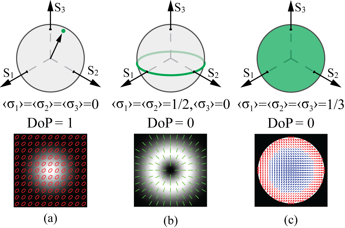 Figure 1
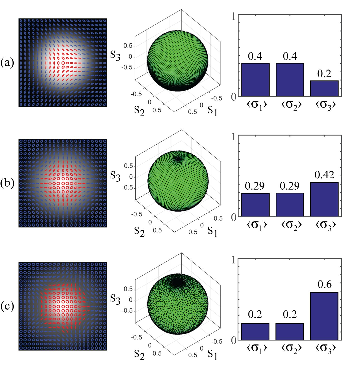 Figure 2
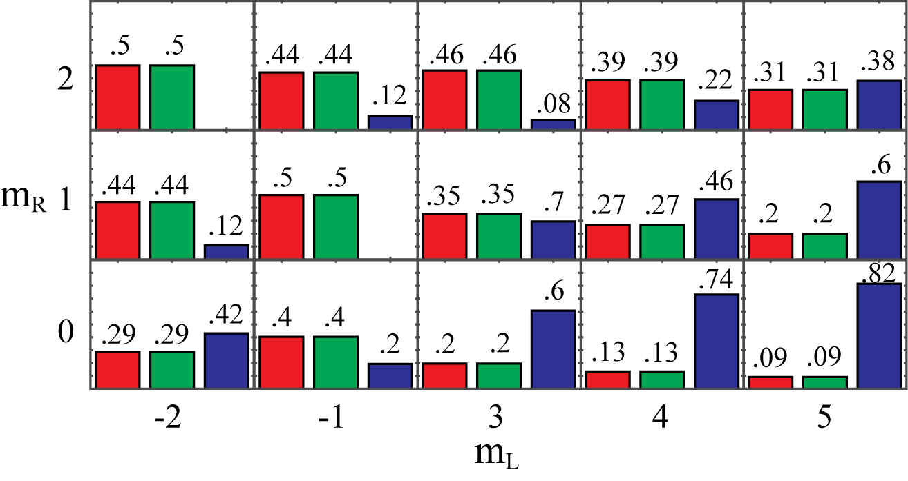 Figure 3
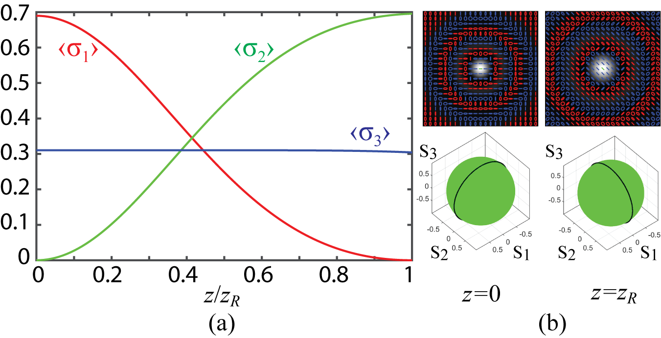 Figure 4
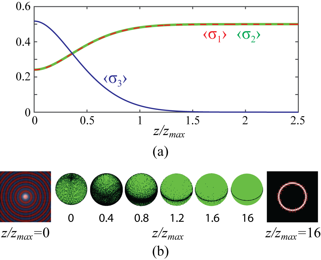 Figure 5
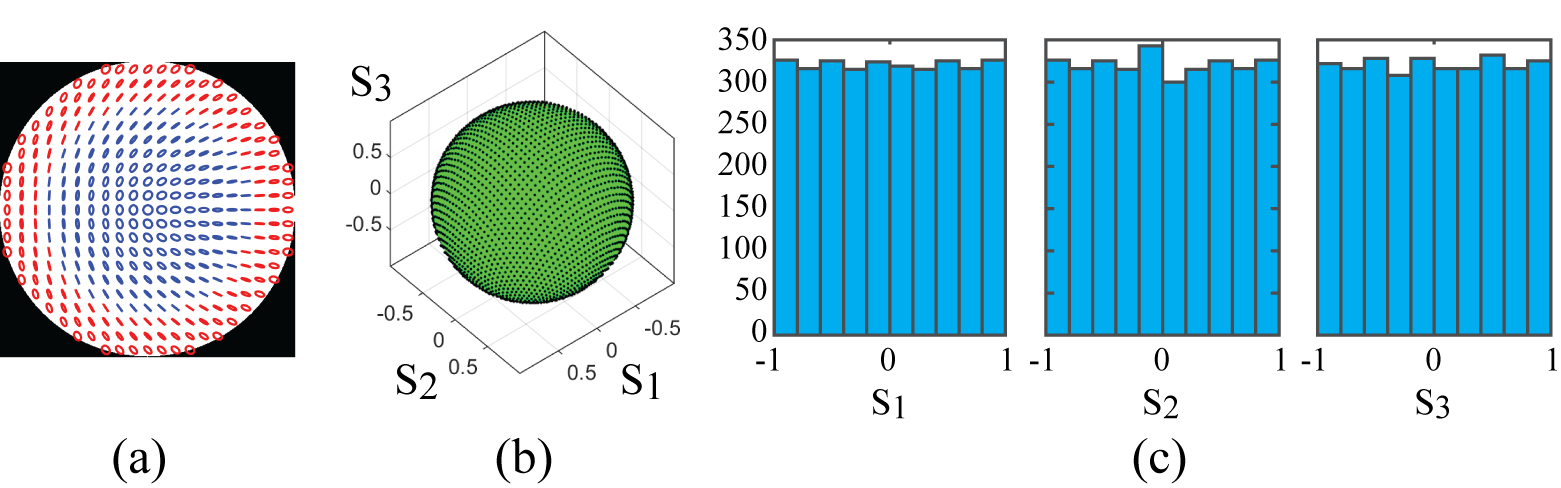 Figure 6
Peer Reviews
No public reviews on file for this paper yet. If you reviewed it on a platform where reviews are public (OpenReview, ICLR, NeurIPS, ICML), you can paste yours below so the community can read it here.
Videos
No videos yet. Explain this paper in a talk, walkthrough, or lecture? Add one.
On the overall polarisation properties of full Poincaré beams
Dorilian Lopez-Mago
Tecnologico de Monterrey
(June 2019
dlopezmago(at)tec.mx)
1 abstract
We analyse the polarisation properties of full Poincaré beams. We consider different configurations, such as Laguerre-Poincaré, Bessel-Poincaré, and Lambert-Poincaré beams. The former is the original Poincaré beam produced by a collinear superposition of two Laguerre-Gauss beams with orthogonal polarisations. For this configuration, we describe the Stokes statistics and overall invariant parameters. Similarly, Bessel-Poincaré beams are produced by the collinear superposition of Bessel beams with orthogonal polarisations. We describe their properties under propagation and show that they behave as a free-space polarisation attractor transforming elliptical polarisations to linear polarisations. We also propose a novel type of full Poincaré pattern, one which is generated by a Lambert projection of the Poincaré sphere on the transverse plane, and hence we call them Lambert-Poincaré. This configuration, contrary to the Laguerre-Poincaré, provides a finite region containing all polarisation states uniformly distributed on the Poincaré sphere.
2 Introduction
Optical beams containing all states of polarisation are known as full Poincaré (FP) beams [1, 2, 3]. Their polarisation properties have attracted attention in beam shaping and singular optics, where they can be used to generate complex topologies such as Möbius strips [4]. Other studies analyse the optical forces arising from the curl of the spin angular momentum [5]. They can be applied in laser cutting, where the flat-top intensity is used to realise a clean cut [6]. Potential applications have been shown for quantum communications [7], single-shot polarimetry [8], and polarisation speckles [9].
Full-Poincaré beams were originally realised by Beckley et al [1]. They are formed by a coherent and collinear superposition of two Laguerre-Gauss (LG) beams with either linear or circular orthogonal polarisations. For the circular basis, two distinct polarisation singularities can be generated, that is, lemon and star singularities. Higher-order FP beams were studied by Galvez et al [2], where superpositions of higher-order LG beams were used to produce the mapping of multiple Poincaré spheres on the transverse plane. Other type of FP beam include the Bessel-Poincaré studied by Shvedov et al [3], which is formed by a superposition of Bessel beams. Similarly, there are Mathieu-Poincaré beams, which are formed by using nondiffracting Mathieu beams [10].
In this work, we describe interesting polarisation properties regarding FP beams. We consider the original FP beams formed with an LG mode basis. We call them Laguerre-Poincaré (LP) to distinguish them from the other structures of interest, which are Bessel-Poincaré (BP) and Lambert-Poincaré (LaP) beams. The latter is realised through a Lambert projection of the Poincaré sphere on the transverse plane. Section 3 describes the Stokes statistics that we use to describe the overall polarisation properties of the FP beams. Inspired by the work of Martínez-Herrero et al [11], we found an invariant parameter that relates the local degree of polarisation with the averaged Stokes parameters. We use this formalism to study the properties of LP beams in section 4. We describe the Stokes variances according to the azimuthal and radial indices and show that higher-order LP beams are predominantly circularly polarised. Furthermore, we study their propagation and describe the evolution of the transverse polarisation distribution as a rotation of the Poincaré sphere. Similarly, section 5 studies the propagation of BP beams and show that they behave as a polarisation attractor [12], which transforms elliptical polarisation states to linear polarisations. Finally, section 6 explains the realisation of the LaP polarisation pattern, which provides a uniform distribution of polarisation states on the Poincaré sphere [13].
3 Global parameters and invariants for the characterisation of space-variant polarised beams
In this section we briefly describe the Stokes statistics in order to stablish basic formulas and notation. The Stokes parameters, with , are determined by six power measurements. Each power measurement is realised after the beam passes through an ideal polariser. The Stokes parameters are defined as [14]
[TABLE]
where is equal to the total power of the beam. is the power transmitted after a horizontal polariser () minus the power transmitted through a vertical polariser (). Similarly, is the power transmitted after a polarizer () minus the power after a polariser (). Finally, measures the difference in power between the right-handed circular component () and the left-handed circular component (). We label these global Stokes parameters as , , , to distinguish them from the space-dependent Stokes parameters defined later.
For space-variant polarised beams, e.g. FP beams, each power measurement is equal to the spatial integration of their respective intensities. For instance
[TABLE]
where is the total intensity of the beam, and are the horizontal and vertical intensity components, respectively. Correspondingly, , , and are the intensity components for , , and . The intensities are measured with a CCD camera whereas the power or flux of energy is measured using a photodetector. To keep the notation simpler, we will disregard the space dependence unless is necessary for clarity.
We define the normalised and space-variant Stokes parameters
[TABLE]
Inspired by the work of Martínez-Herrero et al [11], we consider in our analyses the weighted average of the normalised Stokes parameters, which are given by
[TABLE]
with . Notice that in this definition is equivalent to a density function. In addition, the expected value of the variance is defined as
[TABLE]
We notice that Martínez-Herrero et al used these definitions to characterise space-variant polarised beams in terms of one or two Stokes parameters [11, 15]. However, in this work, we show that considering the three Stokes parameters provide information regarding the distribution of polarisation states over the Poincaré sphere.
In what follows we will repeatedly use the definition
[TABLE]
with . By expanding equation 7, we can write in the alternative form
[TABLE]
We now consider the contribution from the three Stokes parameters. Let us define
[TABLE]
as the total variance of polarisation states. We observe that the first term on the right-hand side,
[TABLE]
is equal to the expected value of the squared of the local degree of polarisation (LDoP), defined as (cf. [11])
[TABLE]
Thus we have that
[TABLE]
Then, the addition of the squared of the average values, turns out to be equal to the squared of the global degree of polarisation (DoP), i.e.
[TABLE]
Therefore, equation 10 can be written as
[TABLE]
By knowing that the global DoP is invariant under propagation through non-polarising optical elements [14], it is convenient to write the previous equation as
[TABLE]
Equation 16 is the first important result of this work. It helps to characterise space-variant polarised beams. The DoP describes the overall state of polarisation whereas the variances describe the spread of the polarisation states on the principal Stokes axes. The DoP has an intuitive interpretation. If we graph the polarisation states on the Poincaré sphere, the DoP resembles the concept of center of mass. Therefore, if the polarisation states span the Poincaré sphere or one of its great circles, it results that , as is the case for FP and cylindrical vector beams. The variances give information about the predominant state of polarisation according to the intensity of the beam. For example, values of means that the beam is circularly polarised in regions where the intensity is more significant.
In the examples that follow, we consider temporally and spatially coherent light beams (e.g. monochromatic laser beams). It means that the light is locally polarised and hence . Therefore , which is written as
[TABLE]
Figure 1 shows examples of the application of the previous equation. We can see that for homogeneously polarised beams and hence . For FP and cylindrical vector beams . Cylindrical vector beams span the equator of the Poincaré sphere, meaning that and (see figure 1(b)). Figure 1(c) shows a LaP beam which uniformly covers the Poincaré sphere and hence .
4 Polarisation properties of Laguerre-Poincaré beams
Under the paraxial approximation an LG beam is written in a cylindrical coordinate system as [16]
[TABLE]
where and are the radial and azimuthal quantum numbers, respectively, and they also determine the order and degree of the generalised Laguerre polynomial . Moreover,
[TABLE]
where is the Rayleigh range, is the wave number, is the beam waist (so is the beam waist at ), is the radius of curvature, and is the Gouy phase. Furthermore, equation 18 is normalised such that .
Laguerre-Poincaré (LP) beams are produced with a coherent and collinear superposition of LG beams with orthogonal polarisations. We consider a circular polarisation basis and use the unit vectors and , which correspond to the right-handed and left-handed circular polarisations, respectively. Thus, an LP beam with circular polarisation basis is given by [2]
[TABLE]
where we consider that both components can have different quantum numbers. Another polarisation basis can be used to generate LP beams, whose difference is observed in the transverse distribution of the polarisation states. The factor of ensures that . Notice that equation 23 does not span all polarisation states for all combinations of and . The cases where one of the components has and the other component has correspond to the first-order LP beams [1]. Higher-order LP beams are generated, for example, with and [6]. Furthermore, cylindrical vector beams correspond to and [17].
Figure 2 shows the properties for different LP beams with both polarisation components carrying a zero radial quantum number (i.e. ). First, second and third columns show the transverse polarisation distribution, the polarisation states visualised on the Poincaré sphere and the Stokes variances (see equation 7), respectively. The calculations were done at the plane with mm and nm. For the transverse polarisation distributions, the gray colormap represents the intensity, whereas the red (blue) ellipses represent polarisation states with right (left) handedness. The graph of the polarisation states on the Poincaré sphere is realised by mapping each pixel of the transverse plane on a unit sphere using the normalised Stokes parameters (see equations 3 to 5).
Figure 2(a) shows a first-order LP beam with a star singularity (). From the transverse pattern, notice that the north hemisphere, the one containing right-handed polarisation states, is located where the intensity of the beam is significant. Specifically, the north hemisphere has about 90 percent of the total power (it was calculated at the radial position that satisfies , which is the location of the equator). Therefore, the left-handed hemisphere covers a region with practically null intensity. This causes that is less significant than and , as shown in the third column.
Figures 2(b) and 2(c) show the results for higher-order LP beams with and (cf. [18]). Since the LG beam radius increases with the azimuthal quantum number due to the factor in equation 18, the overlap between the two LG components decreases for high values of . Therefore, the circular polarisation states are dominant for higher-order LP beams. Notice the accumulation of polarisation states on the poles of the Poincaré sphere. Similarly, the value of becomes more significant than and .
Due to the circular polarisation basis, the results discussed in the previous paragraphs satisfy . Furthermore, notice that in all cases is satisfied. Of course, we can infer similar conclusions according to the polarisation basis that we use. For example, if we use a linear polarisation basis , it is expected that , and the polarisation states on the Poincaré sphere will accumulate on for higher-order modes (and therefore ).
To extend our previous analysis, figure 3 shows more combinations of including negative values. The cases with , where correspond to cylindrical vectors beams. The results confirm that and the predominant variance is for values of (or viceversa ).
Next we study the propagation effects on the Stokes statistics. It has been shown that under propagation the first-order LP beams experience a rotation of their polarisation states equivalent to a rotation of the Poincaré sphere. This rotation depends on the polarisation basis and is due to the Gouy phase (cf. equation 22). For circular polarisation basis the rotation is with respect to the axis (which are the poles of the Poincaré sphere). Since we can expect that this rotation does not change the values of the variances, which is only true for LP beams that cover the Poincaré sphere or its equator. Thus, the rotation does not change the polarisation state distribution on the sphere. Nevertheless, there are cases where the polarisation states cover a great circle of the Poincaré sphere other than the equator. For these cases, we can infer that the rotation will change the values of and . To show this effect, figure 4 shows the Stokes variances for an LP beam with azimuthal quantum numbers and radial numbers . The plot shows the variances as a function of up to one Rayleigh distance. We confirm that remains constant on propagation, but and oscillate with a spatial period equal to . As shown in figure 4(b), the polarisation states at cover the great circle that passes through and . During propagation the states rotates with respect to the axis and at the states cover the great circle that passes through and .
We can summarise the observations for LP beams as follows: (i) cases with and correspond to higher-order LP beams that span all polarisation states. For circular polarisation basis and is predominant if . (ii) Higher-order cylindrical vector beams are given with and . They satisfy and . (iii) For and the polarisation states cover a great circle different than the equator. Under propagation, the variances for the cases (i) and (ii) remain constant, but for (iii) the variances oscillate while remains constant. We remark that in all cases .
5 Polarisation properties of Bessel-Poincaré beams
Here we describe the polarisation properties of BP beams. The spatial modes that we use are paraxial Bessel-Gauss beams instead of nondiffracting Bessel beams. This is with the purpose of describing a beam profile closely related to an experimental realisation. Bessel-Gauss (BG) are described by the expression [19]
[TABLE]
where
[TABLE]
is a Gaussian beam that apodises the Bessel function . The index is the azimuthal quantum number that describes the amount of orbital angular momentum. Furthermore,
[TABLE]
where is tje Rayleigh distance for the GB apodization. However, the distance where the beam behaves as a nondiffracting beam is given by
[TABLE]
The transverse wavevector is related to as .
A first-order BP beam in a circular polarisation basis reads as
[TABLE]
This configuration spans the Poincaré sphere and therefore its . The variances at are equal to and . An interesting difference between BP and LP beams appears on propagation. We notice that for LP beams, the transverse polarisation distribution on propagation changes according to a rigid rotation of the Poincaré sphere (see section 4). It is known that the far-field transverse amplitude of a BG beam corresponds to a ring of intensity. In other words, the angular spectrum of a Bessel beam is a ring in space [20]. Since the ring radius is independent of the azimuthal quantum number [21], the far-field intensity distribution of both components of equation 29 are the same. An equal amplitude superposition means that the resulting polarisation pattern contains linear polarisation states. Therefore, during the propagation of a BP beam, the elliptical polarisation states evolve to linear polarisations.
Figure 5 shows the variances as a function of the propagation distance for a first-order BP beam. In the calculations we use nm, mm, and with . The results confirm our previous comments. Initially, the polarisation states cover the full Poincaré sphere. During propagation, however, the polarisation states are attracted to the equator. This behaviour is compared to a polarisation attractor in optical fibres, where the states are attracted to a particular point or line on the sphere [22]. Notice that at all planes the and due to the circular polarisation basis. However, contrary to the LP beams, the value of is not constant during propagation. It turns out that, since the polarisation states are attracted to the equator, the value of in the far field and . Therefore, the final distribution is a particular case of a vector beam. In the example of figure 5(b) the far-field polarisation distribution is similar to a fractional vector beam of index [23].
6 Polarisation properties of Lambert Poincaré patterns
Here, we show a novel type of FP pattern that covers the Poincaré sphere with a uniform distribution of polarisation states on the sphere. The LP beams have been described as a stereographic projection of the Poincaré sphere on the transverse plane. Nonetheless, this projection maps one of the hemispheres to a region of infinite extension, and thus they are not physically realisable. Instead, we propose a Lambert projection to map the polarisation states on a finite region. Of course, if the field is confined in a finite region, it will diffract during propagation. However, there are several methods to create this pattern in the image plane using spatial light modulators [24, 25, 26].
We define a first-order Lambert-Poincaré pattern using circular polarisation components as
[TABLE]
where is the azimuthal coordinate and is a dimensionless radial coordinate confined in the range . Certainly, higher-order LaP beams can be created by simply adding a larger azimuthal phase variation.
Using the definition for the Stokes parameters in terms of circular polarisation components,
[TABLE]
we can show that and
[TABLE]
Using the previous results it is straightforward to show that , and .
An important property of the LaP pattern is that the polarisation states cover the Poincaré sphere with a uniform distribution [13, 27]. Figure 6(a) shows the transverse polarisation pattern of a first-order LaP containing a lemon singularity (see equation 30). Figure 6(b) shows the polarisation states on the the Poincaré sphere. To show that the polarisation states are uniformly distributed on the sphere, figure 6(c) shows the histogram of polarisation states for the Stokes parameters. The histogram for each Stokes component uses equally spaced bins between and . In our calculations we use a grid of points. The results confirm that the polarisation states are uniformly distributed on the Poincaré sphere.
7 Discussion and conclusions
We have studied the polarisation properties of full Poincaré beams according to the Stokes statistics developed in section 3. Through the use the Stokes variances we have characterised Laguerre-, Bessel- and Lambert- Poincaré patterns. When using a circular polarisation basis, higher-order LP beams showed specific properties according to the radial and azimuthal quantum numbers of its components. On the one hand, equal azimuthal quantum numbers produce a polarisation pattern that covers one great circle of the Poincaré sphere and its Stokes variances change under propagation. On the other hand, dissimilar azimuthal quantum numbers produce full Poincaré patterns whose Stokes statistics are propagation invariant. We also showed that BP beams behave as free-space polarisation attractors, converting elliptical polarisation states to linear polarisation states. In terms of its Stokes statistics, we showed that the variances reach stable values at the far field, where the polarisation pattern is similar to a cylindrical vector beam of fractional order. Therefore, we have shown a method to generate fractional vector beams by propagating a superposition of integer-order Bessel beams. Furthermore, we have presented a LaP polarisation pattern whose polarisation states uniformly cover the Poincaré sphere. This is demonstrated with the histogram of the Stokes parameters which show a flat distribution. The experimental realisation and further properties of LaP patterns are the subject of future work. Finally, we emphasize that the aforementioned Stokes variances can be obtained with current procedures to measure the Stokes parameters. Therefore, they can be used as figures of merit to characterise space-variant polarised beams.
Acknowledgements
We acknowledge support from Consejo Nacional de Ciencia y Tecnología (CONACYT) through the grants: 257517, 280181, 293471, 295239, and APN2016-3140. I also acknowledge helpful discussions with Julio C. Gutiérrez-Vega.
The reference list from the paper itself. Each links out to its DOI / PubMed record.
- 1[1] Beckley A M, Brown T G and Alonso M A 2010 Full Poincaré beams Opt. Express 18 10777–85
- 2[2] Galvez E J, Khadka S, Schubert W H and Nomoto S 2012 Poincaré-beam patterns produced by nonseparable superpositions of Laguerre-Gauss and polarization modes of light Appl. Opt. 51 2925–34
- 3[3] Shvedov V, Karpinski P, Sheng Y, Chen X, Zhu W, Krolikowski W and Hnatovsky C 2015 Visualizing polarization singularities in Bessel-Poincaré beams Opt. Express 23 12444–53
- 4[4] Bauer T et al 2015 Observation of optical polarization Möbius strips Science 347 964–6
- 5[5] Wang L G 2012 Optical forces on submicron particles induced by full Poincaré beams Opt. Express 20 20814–26
- 6[6] Han W, Cheng W and Zhan Q 2011 Flattop focusing with full Poincaré beams under low numerical aperture illumination Opt. Lett. 36 1605–7
- 7[7] Fickler R, Lapkiewicz R, Ramelow S and Zeilinger A 2014 Quantum entanglement of complex photon polarization patterns in vector beams Phys. Rev. A 89 060301
- 8[8] Sivankutty S, Andresen E R, Bouwmans G, Brown T G, Alonso M A and Rigneault H 2016 Single-shot polarimetry imaging of multicore fiber Opt. Lett. 41 2105–8