Tensor Canonical Correlation Analysis with Convergence and Statistical Guarantees
You-Lin Chen, Mladen Kolar, Ruey S. Tsay

TL;DR
This paper develops a tensor canonical correlation analysis framework with convergence guarantees, statistical bounds, and practical algorithms, enabling effective analysis of high-dimensional tensor data in large-scale applications.
Contribution
It introduces a novel tensor CCA method with convergence and statistical guarantees, including scalable algorithms and initialization strategies for real-world tensor data analysis.
Findings
Convergence of the power method for tensor CCA is established.
The proposed method is effective on gene expression and air pollution data.
Scalable algorithms with stochastic gradient descent are validated.
Abstract
In many applications, such as classification of images or videos, it is of interest to develop a framework for tensor data instead of an ad-hoc way of transforming data to vectors due to the computational and under-sampling issues. In this paper, we study convergence and statistical properties of two-dimensional canonical correlation analysis \citep{Lee2007Two} under an assumption that data come from a probabilistic model. We show that carefully initialized the power method converges to the optimum and provide a finite sample bound. Then we extend this framework to tensor-valued data and propose the higher-order power method, which is commonly used in tensor decomposition, to extract the canonical directions. Our method can be used effectively in a large-scale data setting by solving the inner least squares problem with a stochastic gradient descent, and we justify convergence via the…
Click any figure to enlarge with its caption.
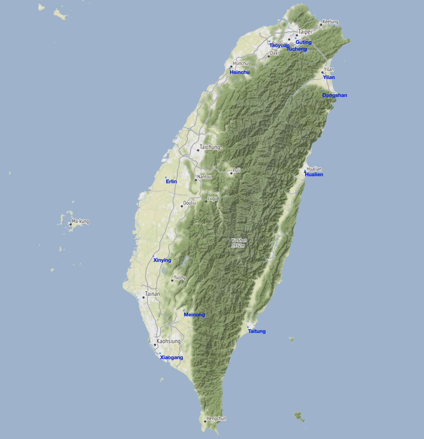 Figure 1
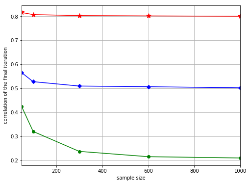 Figure 2
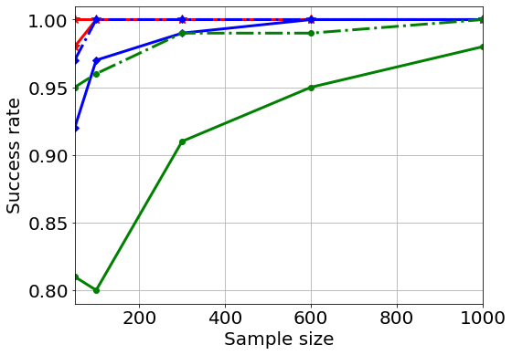 Figure 3
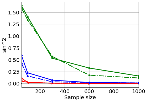 Figure 4
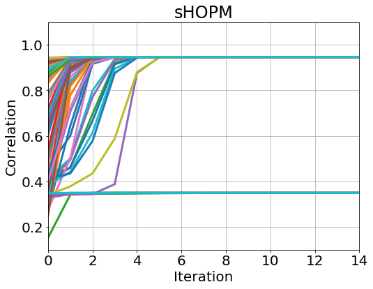 Figure 5
 Figure 6
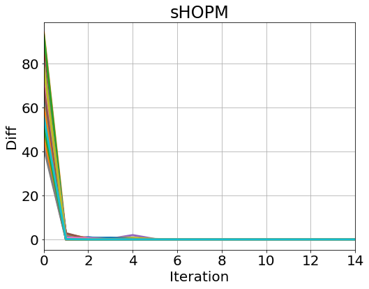 Figure 7
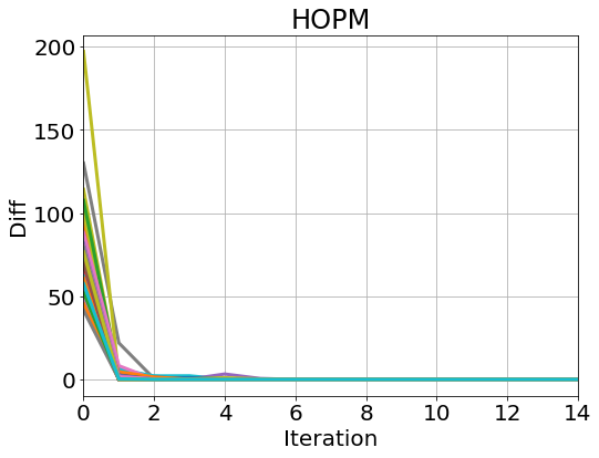 Figure 8
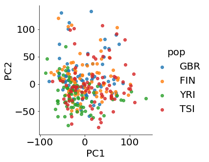 Figure 9
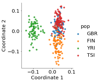 Figure 10
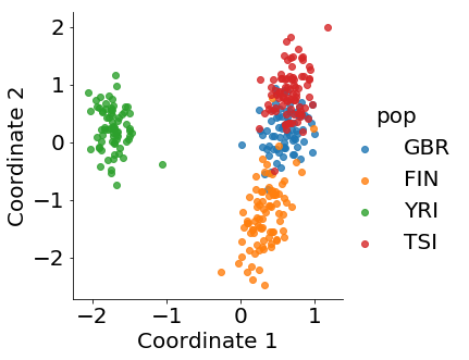 Figure 11
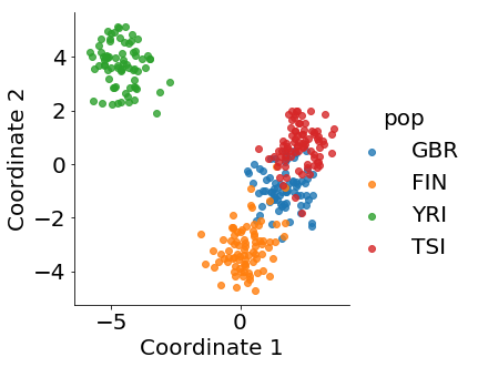 Figure 12
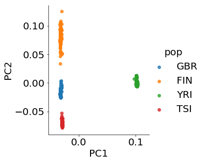 Figure 13
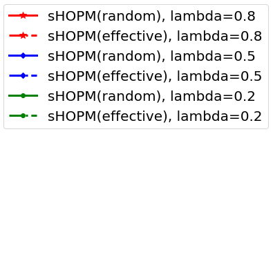 Figure 14
| 1DCCA | TCCA | AppGrad | Rifle | ||
|---|---|---|---|---|---|
| Adelaide | corr (train) | 0.994 | 0.972 | 0.952 | 0.793 |
| corr (test) | 0.904 | 0.969 | 0.844 | 0.836 | |
| time(s) | 0.037 | 0.097 | 3.402 | 131.1 | |
| MINST | corr(train) | 0.962 | 0.939 | 0.953 | 0.953 |
| corr (test) | 0.962 | 0.943 | 0.952 | 0.952 | |
| time(s) | 0.379 | 1.181 | 17.50 | 279.5 | |
| Gene | corr(train) | 1.000 | 0.979 | 0.949 | 0.019 |
| Expression | corr (test) | 0.393 | 0.833 | 0.233 | 0.180 |
| time(s) | 40.32 | 0.089 | 39.94 | 34657 |
| North vs South | South vs East | North vs East |
| 0.888 | 0.817 | 0.904 |
| North | South | |||||||
|---|---|---|---|---|---|---|---|---|
| N vs S | Guting | Tucheng | Taoyuan | Hsinchu | Erlin | Xinying | Xiaogang | Meinong |
| 0.051 | -0.146 | -0.032 | -0.988 | 0.777 | 0.584 | -0.125 | 0.201 | |
| North | East | |||||||
| N vs E | Guting | Tucheng | Taoyuan | Hsinchu | Yilan | Dongshan | Hualien | Taitung |
| 0.627 | 0.671 | 0.215 | 0.331 | 0.895 | -0.051 | 0.441 | 0.044 | |
| South | East | |||||||
| S vs E | Erlin | Xinying | Xiaogang | Meinong | Yilan | Dongshan | Hualien | Taitung |
| 0.625 | 0.142 | 0.596 | 0.483 | 0.511 | -0.145 | 0.303 | 0.791 |
| SO2 | CO | O3 | PM10 | NOx | NO | NO2 | |
|---|---|---|---|---|---|---|---|
| N | 0.001 | 0.478 | -0.322 | -0.132 | -0.417 | 0.604 | 0.333 |
| S | 0.571 | -0.250 | 0.415 | 0.067 | 0.199 | -0.618 | 0.110 |
| N | -0.779 | 0.567 | 0.170 | 0.165 | -0.051 | 0.112 | -0.014 |
| S | -0.027 | -0.566 | 0.402 | 0.409 | 0.212 | 0.010 | -0.552 |
| S | -0.270 | -0.699 | 0.146 | 0.022 | 0.367 | -0.399 | -0.351 |
| E | -0.187 | -0.292 | 0.434 | 0.080 | 0.219 | -0.029 | -0.798 |
| North vs South | South vs East | North vs East | |
|---|---|---|---|
| Winter | 0.940 | 0.904 | 0.930 |
| Summer | 0.889 | 0.821 | 0.914 |
| North | South | |||||||
| N vs S | Guting | Tucheng | Taoyuan | Hsinchu | Erlin | Xinying | Xiaogang | Meinong |
| Winter | 0.423 | 0.060 | 0.078 | 0.901 | -0.925 | -0.344 | 0.161 | -0.024 |
| Summer | 0.400 | -0.277 | -0.189 | -0.853 | 0.834 | 0.435 | 0.206 | 0.270 |
| North | South | |||||||
| N vs E | Guting | Tucheng | Taoyuan | Hsinchu | Yilan | Dongshan | Hualien | Taitung |
| Winter | 0.599 | 0.723 | 0.339 | 0.060 | -0.819 | -0.273 | -0.500 | -0.064 |
| Summer | -0.419 | -0.225 | -0.783 | -0.402 | -0.843 | -0.195 | -0.465 | -0.188 |
| South | East | |||||||
| S vs E | Erlin | Xinying | Xiaogang | Meinong | Yilan | Dongshan | Hualien | Taitung |
| Winter | 0.961 | -0.061 | 0.116 | 0.244 | -0.462 | -0.143 | -0.751 | -0.449 |
| Summer | 0.354 | 0.798 | 0.300 | 0.386 | 0.733 | -0.363 | 0.332 | 0.469 |
| SO2 | CO | O3 | PM10 | NOx | NO | NO2 | |
|---|---|---|---|---|---|---|---|
| N(Winter) | 0.122 | 0.672 | -0.176 | -0.084 | 0.298 | -0.083 | -0.633 |
| S(Winter) | 0.228 | 0.805 | 0.357 | 0.071 | 0.292 | -0.242 | 0.152 |
| N(Summer) | -0.540 | -0.344 | 0.532 | 0.060 | 0.263 | -0.480 | 0.066 |
| S(Summer) | -0.000 | 0.136 | -0.360 | 0.003 | 0.232 | 0.740 | -0.499 |
| N(Winter) | 0.477 | 0.330 | -0.247 | -0.078 | 0.397 | -0.430 | -0.504 |
| E(Winter) | -0.558 | -0.228 | 0.333 | 0.150 | 0.417 | -0.484 | -0.307 |
| N(Summer) | -0.111 | 0.113 | 0.074 | 0.188 | 0.450 | -0.283 | -0.807 |
| E(Summer) | 0.272 | -0.371 | 0.127 | 0.209 | 0.099 | 0.473 | -0.704 |
| S(Winter) | 0.404 | 0.027 | -0.263 | -0.019 | -0.627 | 0.392 | 0.469 |
| E(Winter) | -0.304 | -0.523 | 0.171 | 0.077 | 0.280 | -0.712 | -0.115 |
| S(Summer) | -0.608 | -0.103 | 0.174 | 0.009 | 0.455 | -0.300 | -0.541 |
| E(Summer) | -0.111 | 0.024 | 0.269 | 0.046 | 0.262 | 0.619 | -0.679 |
| All | Day(10am-3pm) | Evening(6pm-11pm) |
| 0.973 | 0.885 | 0.714 |
| Mon. | Tue. | Wed. | Thu. | Fri. | Sat. | Sun. | |
|---|---|---|---|---|---|---|---|
| Whole day | 0.240 | 0.413 | 0.385 | 0.436 | 0.420 | 0.441 | 0.244 |
| Day (10am-3pm) | 0.375 | 0.437 | 0.440 | 0.432 | 0.396 | 0.299 | 0.198 |
| Evening (6pm-11pm) | 0.195 | 0.325 | 0.528 | 0.160 | -0.323 | -0.584 | -0.322 |
| 0 | 1 | 2 | 3 | ||||
|---|---|---|---|---|---|---|---|
| -0.080 | -0.076 | -0.104 | -0.104 | -0.061 | -0.021 | 0.021 | 0.067 |
| 4 | 5 | 6 | 7 | ||||
| 0.099 | 0.121 | 0.12 | 0.075 | -0.002 | -0.086 | -0.129 | -0.144 |
| 8 | 9 | 10 | 11 | ||||
| -0.155 | -0.156 | -0.151 | -0.125 | -0.064 | 0.002 | 0.066 | 0.116 |
| 12 | 13 | 14 | 15 | ||||
| 0.145 | 0.174 | 0.179 | 0.177 | 0.206 | 0.238 | 0.262 | 0.284 |
| 16 | 17 | 18 | 19 | ||||
| 0.281 | 0.227 | 0.121 | -0.054 | -0.231 | -0.237 | -0.214 | -0.206 |
| 20 | 21 | 22 | 23 | ||||
| -0.135 | -0.071 | -0.058 | -0.069 | -0.080 | -0.055 | -0.004 | -0.062 |
| 10 | 11 | 12 | 13 | 14 | |||||
|---|---|---|---|---|---|---|---|---|---|
| -0.611 | -0.385 | -0.165 | -0.084 | 0.012 | 0.198 | 0.281 | 0.264 | 0.321 | 0.391 |
| 18 | 19 | 20 | 21 | 22 | |||||
| 0.676 | 0.523 | 0.384 | 0.275 | 0.167 | 0.109 | 0.066 | 0.033 | 0.025 | 0.029 |
Peer Reviews
No public reviews on file for this paper yet. If you reviewed it on a platform where reviews are public (OpenReview, ICLR, NeurIPS, ICML), you can paste yours below so the community can read it here.
Code & Models
Videos
No videos yet. Explain this paper in a talk, walkthrough, or lecture? Add one.
Taxonomy
TopicsTensor decomposition and applications · Sparse and Compressive Sensing Techniques · Advanced Neuroimaging Techniques and Applications
Tensor Canonical Correlation Analysis with Convergence and Statistical Guarantees
You-Lin Chen
Department of Statistics, University of Chicago
and
Mladen Kolar and Ruey S. Tsay
University of Chicago, Booth School of Business
Abstract
In many applications, such as classification of images or videos, it is of interest to develop a framework for tensor data instead of an ad-hoc way of transforming data to vectors due to the computational and under-sampling issues. In this paper, we study convergence and statistical properties of two-dimensional canonical correlation analysis (Lee and Choi, 2007) under an assumption that data come from a probabilistic model. We show that carefully initialized the power method converges to the optimum and provide a finite sample bound. Then we extend this framework to tensor-valued data and propose the higher-order power method, which is commonly used in tensor decomposition, to extract the canonical directions. Our method can be used effectively in a large-scale data setting by solving the inner least squares problem with a stochastic gradient descent, and we justify convergence via the theory of Lojasiewicz’s inequalities without any assumption on data generating process and initialization. For practical applications, we further develop (a) an inexact updating scheme which allows us to use the state-of-the-art stochastic gradient descent algorithm, (b) an effective initialization scheme which alleviates the problem of local optimum in non-convex optimization, and (c) a deflation procedure for extracting several canonical components. Empirical analyses on challenging data including gene expression and air pollution indexes in Taiwan, show the effectiveness and efficiency of the proposed methodology. Our results fill a missing, but crucial, part in the literature on tensor data.
Keywords: Canonical correlation analysis, Deflation, Higher-order power method, Non-convex optimization, Lojasiewicz’s inequalities, Tensor decomposition.
1 Introduction
Canonical Correlation Analysis (CCA) is a widely used multivariate statistical method that aims to learn a low dimensional representation from two sets of data by maximizing the correlation of linear combinations of the sets of data (Hotelling, 1936). The two data sets could be different views (deformation) of images, different measurements of the same object or data with labels. CCA has been used in many applications, ranging from text and image retrieval (Mroueh et al., 2016) and image clustering (Jin et al., 2015), to various scientific fields (Hardoon et al., 2004). In contrast to principal component analysis (PCA) (Pearson, 1901), which is an unsupervised learning technique for finding low dimensional data representation, CCA benefits from the label information (Sun and Chen, 2007), other views of data, or correlated side information as in multi-view learning (Sun, 2013).
In this paper, we study CCA in the context of matrix valued and tensor valued data. Matrix valued data have been studied in (Gupta and Nagar, 2000; Kollo and von Rosen, 2005; Werner et al., 2008; Leng and Tang, 2012; Yin and Li, 2012; Zhao and Leng, 2014; Zhou and Li, 2014), while tensor valued data in (Ohlson et al., 2013; Manceur and Dutilleul, 2013; Lu et al., 2011). Practitioners often apply CCA to such data by first converting them into vectors, which destroys the inherent structure present in the samples, increases the dimensionality of the problem as well as the computational complexity. Lee and Choi (2007) proposed a two-dimensional CCA (2DCCA) to address these problems for matrix valued data. 2DCCA preserves data representation and alleviates expensive computation of high dimensional data that arises from vectorizing. However, convergence properties of the algorithm proposed in Lee and Choi (2007) are still not known.
We present a power method that can solve the 2DCCA problem and present a natural extension of 2DCCA to tensor-valued data. The higher-order power method (HOPM) and its variant are introduced for solving the resulting optimization problem. HOPM is a common algorithm for tensor decomposition (Kolda and Bader, 2009; De Lathauwer et al., 2000a, b), with convergence properties intensely studied in recent years (Wen et al., 2012; Uschmajew, 2015; Xu and Yin, 2013; Li et al., 2015; Guan et al., 2018). However, these convergence results are not directly applicable to CCA for the tensor data. One particular reason is that the CCA constraints do not imply the identifiability. It is also possible that iterates of HOPM get trapped in a local maximum with random initialization. In order to establish convergence of HOMP for the tensor valued CCA problem, a probabilistic model of 2DCCA is introduced. Under this model, we can characterize covariance and cross-covariance matrix explicitly, which shows HOPM provably converges to the optimum of the objective function provided that the initialization is close enough to optimum. For a model-free setting, we introduce a variant of HOPM with the simple projection and show the equivalence. This insight of the equivalence as well as the theory of analytical gradient flows and Lojasiewicz gradient inequality provides solution to prove the convergence bound. There are two implications from this result. First, a deflation procedure which does not require any singular value decomposition is given for extracting multiple canonical components. Second, the theorem guarantees existence and uniqueness of the limit of iterates of HOPM with the arbitrary initialization. This means the HOPM converges even when initialized poorly.
1.1 Main Contributions
We make several contributions in this paper.
First, we interpret 2DCCA (Lee and Choi, 2007) as a non-convex method for the low rank tensor factorization problem. This allows us to formulate a tensor extension of 2DCCA, which we term tensor canonical correlation analysis (TCCA). We discuss convergence and statistical property under a probabilistic model. In the literature, Kim et al. (2007) and Luo et al. (2015) discuss tensor extension of CCA in different settings. The former stresses correlation between each mode, while the latter discusses CCA when multiple views of data are available. None of them provide theoretical justifications or efficient algorithms. See Section 1.2 for more discussions.
Second, we develop the higher-order power method and its variant for solving the TCCA problem. One obstacle in analysis of tensor factorization is unidentifiability. To circumvent this difficulty and seek further numerical stability, we propose a variant of HOPM called Simple HOPM (sHOPM), which uses a different normalization scheme, and show both are equivalent with same initialization. See Proposition 7 for a formal statement. Through this insight and borrowing tools from tensor factorization, we show that HOPM converges with arbitrary initial points.
Third, we consider several practical issues that arise in analysis of real data. We provide an effective initialization scheme to reduce the probability of the algorithm getting trapped in a poor local optimum and develop a faster algorithm for large scale data. Furthermore, we discuss a deflation procedure which is used to extract multiple canonical components without any decomposition.
Finally, we apply our method to several real data sets, including gene expression data, air pollution data, and electricity demands. The results demonstrate that our method is efficient and effective even in the extremely high-dimensional setting and can be used to extract useful and interpretable features from the data.
1.2 Related Work
Two papers in the literature are closely related to our tensor canonical correlation analysis. Luo et al. (2015) consider multiple-view extension of CCA, which results in a tensor covariance structure. However, they only consider the vector-valued data, so the vectorization is still required in their setting. Kim et al. (2007) extend CCA to the tensor data, focusing on 3 dimensional videos, but only consider joint space-time linear relationships, which is neither the low-rank approximation of CCA nor the extension of 2DCCA. Moreover, none of the aforementioned papers provide convergence analysis, as we detail in Section 3.1 and Section 4.3. Furthermore, 2DCCA (Lee and Choi, 2007) and other 2D extensions proposed in the literature (Yang et al., 2004; Ye et al., 2004; Zhang and Zhou, 2005; Yang et al., 2008) also lack rigorous analysis.
Various extensions of CCA are available in the literature. Kernel method aims to extract nonlinear relations via implicitly mapping data to a high-dimensional feature space (Hardoon et al., 2004; Fukumizu et al., 2007). Other nonlinear transformations have been considered to extract more sophisticated relations embedded in the data. Andrew et al. (2013) utilized neural networks to learn nonlinear transformations, Michaeli et al. (2016) used Lancaster’s theory to extend CCA to a nonparametric setting, while Lopez-Paz et al. (2014) proposed a randomized nonlinear CCA, which uses random features to approximate a kernel matrix. Bach and Jordan (2006) and Safayani et al. (2018) interpreted CCA as a latent variable model, which allows development of an EM algorithm for parameter estimation. In the probabilistic setting, Wang et al. (2016b) developed variational inference. In general, nonlinear extensions of CCA often lead to complicated optimization problems and lack rigorous theoretical justifications.
Our work is also related to scalable methods for solving the CCA problem. Although CCA can be solved as a generalized eigenvalue problem, computing singular value (or eigenvalue) decomposition of a large (covariance) matrix is computationally expensive. Finding an efficient optimization method for CCA remains an important problem, especially for large-scale data, and has been intensively studied (Yger et al., 2012; Ge et al., 2016; Allen-Zhu and Li, 2017; Xu et al., 2018; Fu et al., 2017; Arora et al., 2017; Bhatia et al., 2018). Ma et al. (2015) and Wang et al. (2016a) are particularly related to our work. Wang et al. (2016a) formulated CCA as a regularized least squares problem solved by stochastic gradient descent. Ma et al. (2015) developed an augmented approximate gradient (AppGrad) scheme to avoid computing the inverse of a large matrix. Although AppGrad does not directly maximize the correlation in each iteration, it can be shown that the CCA solution is a fixed point of the AppGrad scheme. Therefore, if the initialization is sufficiently close to the global CCA solution, the iterates of AppGrad would converge to it.
1.3 Organization of the paper
In Section 2, we define basic notations and operators of multilinear algebra and introduce CCA and the Lojasiewicz inequality. We present the 2DCCA and its convergence analysis in Section 3. Then we extend 2DCCA to tensor data and include a study of HOPM as well as a deflation procedure in Section 4. Section 5 deals with practical considerations including an inexact updating rule and effective initialization. Numerical simulations verifying the theoretical results and applications to real data are given in Section 6. All technical proofs can be found in the appendix.
2 Preliminaries
In this section, we provide the necessary background for the subsequent analysis, including some basic notations and operators in multilinear algebra. The Lojasiewicz inequality and the associated convergence results are presented in Section 2.2, and the canonical correlation analysis is briefly reviewed in Section 2.3.
2.1 Multilinear Algebra and Notation
We briefly introduce notation and concepts in multilinear algebra needed for our analysis. We recommend Kolda and Bader (2009) as the reference. We start by introducing the notion of multi-dimensional arrays, which are also called tensors. The order of a tensor, also called way or mode, is the number of dimensions the tensor has. For example, a vector is a first-order tensor, and a matrix is a second-order tensor. We use the following convention to distinguish between scalars, vectors, matrices, and higher-order tensors: scalars are denoted by lower-case letters (), vectors by upper-case letters (), matrices by bold-face upper-case letters (), and tensors by calligraphic letters (). For an -mode tensor , we let its -th element be or .
Next, we define some useful operators in multilinear algebra. Matricization, also known as unfolding, is a process of transforming a tensor into a matrix. The mode- matricization of a tensor is denoted by and arranges the mode- fibers to be the columns of the resulting matrix. More specifically, tensor element maps to matrix element , where with . The vector obtained by vectorization of is denoted by . The Frobenius norm of the tensor is defined as , where is the inner product defined on two tensors , and given by
[TABLE]
The mode- product of a tensor with a matrix is a tensor of size defined by
[TABLE]
The outer product of vectors , …, is an -order tensor defined by
[TABLE]
The Kronecker product of two matrices and is an matrix given by . We call a rank-one tensor if there exist vectors such that . Given samples , it is also useful to define the data tensor with elements .
2.2 Convergence Analysis via Lojasiewicz Inequality
There are two common approaches for establishing convergence of non-convex methods. One assumes that the initial points lie in a convergence region in which the optimization procedure converges to the global optimum. For certain problems, there are effective initialization schemes that provide, with high probability, an initial point that is close enough (within the convergence region) to the global optimum. We provide this type of analysis in Section 3.2 and an effective initialization scheme in Section 5.2.
Another approach is based on the theory of analytical gradient flows, which allows establishing convergence of gradient descent based algorithms for difficult problems, such as, non-smooth, non-convex, or manifold optimization. This approach is also useful for problems arising in tensor decomposition where the optimum set is not compact and isolated. For example, in the case of PCA or CCA problems, the optimum set is a low dimensional subspace or manifold. The advantage of this approach is that it can be applied to study convergence to all stationary points, without assuming a model for the data generating process. The drawback of the approach is that the convergence rate on a particular problem depends on the Lojasiewicz exponent in Lemma 1 below, which is hard to explicitly compute. However, Liu et al. (2018) recently showed that the Lojasiewicz exponent at any critical point of the quadratic optimization problem with orthogonality constraint is , which leads to linear convergence of gradient descent. Li and Pong (2018) developed various calculus rules to deduce the Lojasiewicz exponent.
The method of Lojasiewicz gradient inequality allows us to study an optimization problem
[TABLE]
where may not be convex, and we apply a gradient based algorithm for finding stationary points. The key ingredient for establishing linear or sublinear convergence rate is the following Lojasiewicz gradient inequality (Łojasiewicz, 1965).
Lemma 1** (Lojasiewicz gradient inequality).**
Let be a real analytic function on a neighborhood of a stationary point in . Then, there exist constants and the Lojasiewicz exponent , such that
[TABLE]
where is in some neighborhood of .
See Absil et al. (2005) and references therein for the proof and discussion. Since the objective function appearing in the CCA optimization problem is a polynomial, we can use the Lojasiewicz gradient inequality in our convergence analysis. Suppose is a sequence of iterates produced by a descent algorithm that satisfy the following assumptions:
** Primary descent condition:**
there exists such that, for a sufficiently large , it holds that
[TABLE]
** Stationary condition:**
for a sufficiently large , it holds that
[TABLE]
** Asymptotic small step-size safeguard:**
there exists such that, for a large enough , it holds that
[TABLE]
Then, we have the following theorem which is the main tool we use in our analysis and its proof can be found in Schneider and Uschmajew (2015).
Lemma 2** (Schneider and Uschmajew (2015)).**
Under the condition of Lemma 1 and assumptions (A1) and (A2), if there exists a cluster point of the sequence satisfying (L), then is the limit of the sequence, i.e., . Furthermore, if (A3) holds, then
[TABLE]
for some . Moreover, .
It is not hard to see that the gradient descent iterates for a strongly convex and smooth function satisfy conditions (A1)-(A3) and Lojasiewicz gradient inequality. Moreover, if one can show that Lojasiewicz’s inequality holds with for the set of stationary points, then linear convergence to stationary points can be established (Liu et al., 2018). In fact, they related Lojasiewicz’s inequality to the following error bound (Luo and Tseng, 1993):
[TABLE]
where and is in the set of stationary points. Karimi et al. (2016) proved that these two conditions actually imply quadratic growth:
[TABLE]
where . This means that is strongly convex when is close to a stationary point. Those local conditions are useful in non-convex and even non-smooth, non-Euclidean setting. See Karimi et al. (2016) and Bolte et al. (2017) for additional discussion.
2.3 Canonical Correlation Analysis
Unless otherwise stated, we assume that all random elements in this paper are zero-mean. We first review the classical canonical correlation analysis in this section. Consider two multivariate random vectors and . The canonical correlation analysis aims to maximize the correlation between the projections of two random vectors and can be formulated as the following maximization problem
[TABLE]
The above optimization problem can be written equivalently in the following constrained form
[TABLE]
where, under the zero-mean assumption, , , and . Using the standard technique of Lagrangian multipliers, we can obtain and by solving the following generalized eigenvalue problem
[TABLE]
where and is the Lagrangian multiplier. In practice, the data distribution is unknown, but i.i.d. draws from the distribution are available. We can estimate the canonical correlation coefficients by replacing the expectations with sample averages, leading to the empirical version of the optimization problem.
3 Two-Dimensional Canonical Correlation Analysis
Lee and Choi (2007) proposed two-dimensional canonical correlation analysis (2DCCA), which extends CCA to matrix-valued data. The naive way of dealing with matrix-valued data is to reshape each data matrix into a vector and then apply CCA. However, this naive preprocessing procedure breaks the structure of the data and introduces several side effects, including increased computational complexity and larger amount of data required for accurate estimation of canonical directions. To overcome this difficulty, 2DCCA maintains the original data representation and performs CCA-style dimension reduction as follows. Given two data matrices , 2DCCA seeks left and right transformations, , that maximize the correlation between and and can be formulated as
[TABLE]
where we assume have the same shape for simplicity.
To solve the problem above, for fixed and , and are random vectors and and can be obtained using any CCA algorithm. Similarly we can switch the roles of variables and fix and . Thus, the algorithm iterates between updating and with and fixed and updating and with and fixed.
To the best of our knowledge, no clear interpretation on why 2DCCA can improve the classification results, how the method is related to data structure, nor rigorous convergence analysis exists for 2DCCA. We address these issues, by first noting that the 2DCCA problem in (4) can be expressed as
[TABLE]
where denotes the trace of a matrix. Therefore, we can treat 2DCCA as the CCA optimization problem with the low-rank restriction on canonical directions. Furthermore, formulating the optimization problem as in (5) allows us to use techniques based on the Burer-Monteiro factorization (Chen and Wainwright, 2015; Park et al., 2018, 2017; Sun and Dai, 2017; Haeffele et al., 2014) and non-convex optimization (Yu et al., 2018; Zhao et al., 2015; Yu et al., 2017; Li et al., 2019; Yu et al., 2019).
3.1 Probabilistic model of 2DCCA
We now introduce a probabilistic model of 2DCCA, which is closely related to factor models appearing in the literature (Virta et al., 2017, 2018; Jendoubi and Strimmer, 2019). Consider two random matrices, , distributed according to the following probabilistic model
[TABLE]
where , , are random matrices of appropriate dimensions, satisfying , and are fixed matrices. Note that this probabilistic 2DCCA model is different from the one in Safayani et al. (2018) due to different noise structure. We refer to the 2DCCA model in Safayani et al. (2018) as a 2D-factor model and to our model in (6) as the probabilistic model of 2DCCA or simply, a p2DCCA model.
In practice, the noise structure appearing in the p2DCCA model is more natural than that in the 2D-factor model. Consider the example of image data where and are images of the same object with different illumination conditions. The 2D-factor model implies additive error on images, which is unrealistic. In contrast, the p2DCCA model considers latent variable , which corresponds to the common representations, while and are different views obtained from the transformation defined by . can represent the magnitude of illumination, the angle of a face, or the gender of a person. The p2DCCA model assumes the error is on the common representation, e.g., the magnitude of illumination. This exactly fits the description of our example and the explanations of latent models. Hence, it is reasonable to assume that ’s elements are independent or uncorrelated, which admits a causal interpretation for the latent variables that data satisfy the principle of independent mechanisms in causal inference Peters et al. (2017). That is, the causal generative process of a hidden variables is composed of autonomous modules that do not influence each other. In contrast, the factor model can be better suited for the situations where the additive error is a natural assumption, e.g., time series data (Wang et al., 2019; Chen and Chen, 2017; Chen et al., 2019).
Note that we can always apply CCA to the data after converting them to vectors. However, this leads to -by- matrix inversion, while by exploiting the structure in 2DCCA we only need to solve -by- and -by- matrix inversion, which decreases requirement for memory and computation. One drawback of the 2DCCA method is that the problem is non-convex and it is possible to get stuck in local optimums even if we have infinite samples, that is, at the population level. We can see why this phenomenon exists in the next section.
3.2 Convergence Analysis
In this section, we discuss the convergence behavior of power method for 2DCCA. Suppose that
[TABLE]
where . While we assume that the elements of are uncorrelated and real data may not be generated from this model, this probabilistic model can approximately describe data with some “low rank structure.” For simplicity, we assume the approximate error is zero, but it is possible that the analysis can be extended to the approximate case.
The solution to 1DCCA problem can be obtained as follows. Given covariances and a cross-covaraince , if are the first left and right singular vectors of , respectively, then the first 1DCCA components are and . The following proposition characterizes optimums of 1DCCA and 2DCCA. The proof is deferred to Appendix A.1.
Proposition 3**.**
* and admit a low-rank structure. That is, there exist such that*
[TABLE]
Moreover, the optimums of 2DCCA (4) and 1DCCA (2) coincide.
Thus, we have the closed form of global optimum of 2DCCA under the p2DCCA model. Under the model assumption (6), for , letting
[TABLE]
where
[TABLE]
we show the power method of 2DCCA converges to the global optimum in the population level provided that the initial point is close enough to the global optimum.
Theorem 4**.**
Consider the following power method iterations for the left and right loading vectors in 2DCCA:
[TABLE]
Define and for . Suppose initialization vectors and satisfy, for
[TABLE]
Then
[TABLE]
for , where is a large enough constant depending on the initial values.
The proof is in Appendix A.2. From the proof, we can see that without careful initialization, the power method may converge to arbitrary points. Our analysis can be extended to -2DCCA and higher order cases where is the number of components of left and right loading matrices.
Next, we establish finite-sample bound. Suppose we have i.i.d. data sampled from the data generating process (6). For , let
[TABLE]
where are defined in (9). The regularization is necessary for finite sample estimation, since data have low rank structure and CCA involves matrix inversion that can amplify noise arbitrarily. We state the sample version of the convergence theorem next.
Theorem 5**.**
Suppose that almost surely. Consider the following power method iterations for the left and right loadings in 2DCCA:
[TABLE]
for . Define
[TABLE]
and for . Suppose initialization satisfies such that for all
[TABLE]
Then, with probability , we have
[TABLE]
for , provided that , where are constants depending on initialization and is a small constant depending on initialization, , ,, and . In particular, if , we obtain consistency.
The proof is detailed in Appendix A.3. The key ingredient we use in the proof is the robustness analysis of power method. Using the concentration bound of bounded random matrices, with careful initialization, we can also prove the power method converges to optimum with high probability as long as the sample size is large enough.
4 Tensor Canonical Correlation Analysis
In this section, we extend CCA to the tensor-valued data and the higher-order power method and its variant. We also establish convergence results without any model assumption. The last part discusses how to find multiple canonical variables.
4.1 Canonical Correlation Analysis with Tensor-valued Data
We are ready to present the problem of tensor canonical correlation analysis, which is a natural extension of 2DCCA. Consider two zero-mean random tensors and . Note that, for simplicity of presentation, we assume the two random tensors and have the same mode and shape. This assumption is not needed in the analysis or the algorithm. TCCA seeks two rank-one tensors and that maximize the correlation between and ,
[TABLE]
Since the population distribution is unknown, by replacing covariance and cross-covariance matrices by their empirical counterparts, we get the empirical counterpart of the optimization problem in (12)
[TABLE]
where is the sample correlation defined as
[TABLE]
and are the samples from the unknown distributions of . The following empirical version of residual form of the problem (12) will be useful for developing efficient algorithms
[TABLE]
This formulation reveals that TCCA is related to tensor decomposition. Furthermore, the sub-problem obtained by fixing all components of except for components or is equivalent to the least squares problem. This allows us to use the state-of-the-art solvers based on (stochastic) gradient descent that are especially suitable for large-scale data (Wang et al., 2016a) and develop computationally efficient algorithms for CCA with tensor data proposed in Section 5.
4.2 Higher-order Power Method
The power method is a practical tool for finding the leading eigenvector of a matrix, which is used in tensor factorization. There are many interpretations for the power method and here we show that HOPM solve the stationary condition of a certain Lagrange function.
The Lagrange function associated with the optimization problem in (14) is
[TABLE]
where and are the Lagrange multipliers. Minimizing the above problem in one component of , with the other components of fixed, leads to a least squares problem. Define the partial contraction of with all component of except as
[TABLE]
Similar notation is defined for the partial contraction of . With this notation, we set the gradients and equal to zero, which yields the following stationary conditions
[TABLE]
Combining the two equations with similar stationary conditions for , we obtain the following updating rule
[TABLE]
where are the pseudo inverses of , respectively. The update (16) is in the form of the power method on matrices and (Regalia and Kofidis, 2000; Kolda and Bader, 2009). Cyclically updating each component yields the higher-order power method, which is detailed in Algorithm 1 and similar to the one in Wang et al. (2017).
In a CCA problem, only the projection subspace is identifiable, since the correlation is scale invariant. Same is true in PCA and partial least squares (PLS) problems in both matrix and tensor cases (Arora et al., 2012; Uschmajew, 2015; Gao et al., 2017). Therefore, normalization steps restricting canonical variables are only important for numerical stability. The major difference between PCA and CCA is that the normalization steps are essential in HOPM for preventing and iterates from converging to zero quickly.
The key insight is that different regularization schemes actually generate the same sequence of correlation values for one component CCA, which is stated formally in Proposition 7. This insight allows us to solve TCCA via a variant, called Simple HOPM (sHOPM), which uses the Euclidean norm as regularization, and prove existence and uniqueness of the limit of iterates of HOPM. See Algorithm 1 for details. The Euclidean norm provides the simplest form of regularization and does not depend on the data, which increases the numerical stability as well as decreases computational costs. One of the reasons for numerical instability of HOPM comes from rank deficiency of the covariance matrices and , which commonly arises in CCA due to the low rank structure of the data and undersampling. The numerical stability can also be improved by adding a regularization term to the empirical covariance matrix.
Another major problem is related to identifiability. Observe that if and are a stationary point, then and are also a stationary point for any non-zero constant . In particular, the optimum set is not isolated nor compact. In this case, it is possible that the iteration sequence diverges, even while approaching the stationary set. This is the main difficulty in the analysis of convergence in tensor factorization. Moreover, any component approaching zero or infinity causes numerical instability. One way to overcome identifiability is by adding a penalty function to balance magnitude of each component. However, using this approach, one cannot find the exact solution when updating each component and the whole optimization process is slowed down. We show that HOPM for one component CCA is equivalent to projecting each component to a compact sphere, so those remedies are unnecessary.
The projection to the unit sphere is not the projection onto the constraint in (14). Therefore, we need to address the question whether two different projections generate two different sequences of iterates that have different behaviors. In what follows, we explain how to answer the above question by introducing a new objective function. Consider the modified loss (potential) function
[TABLE]
where we have added two extra normalization variables to the components of and . This type of potential function appears in the literature on PCA and tensor decomposition. For example, the following two optimization problems are equivalent for the problem of finding the best rank-one tensor approximation of
[TABLE]
HOPM represents the latter problem which is convex with respect to each component , and sHOPM represents the former optimization problem which is no longer a convex problem with respect to and . In the first formula, it is obvious that once is found, then so is . Therefore, we may ignore in the optimization procedure, but considering this form is convenient for the analysis.
The following proposition shows how the sHOPM relates to (17):
Proposition 6**.**
Suppose we have the dynamical iterates of sHOPM as follows
[TABLE]
Then (18) satisfies the stationary condition of (17).
The proof follows by simple calculation and is given in Appendix A.4. This gives a justification for sHOPM, which alternatively produces iterates that satisfy the stationary condition of (17). Since we introduced the normalization variables , we changed the subproblem to a noncovex problem, we do not know if sHOPM increases the correlation in each iteration or not. To answer this, the following proposition shows that HOPM and sHOPM generate iterates with the same correlation in each iteration based on the fact that correlation is scale invariant. In particular, this shows that HOPM increases the correlation each time it solves the TCCA problem in (14) regardless of regularization.
Proposition 7**.**
Let , be the iterates generated by HOPM option I and II with the same starting values, respectively. Then, it holds that
[TABLE]
and . Moreover, if is a critical point of the modified loss and , then is a critical point of the original loss .
Note that it is easier to understand the power method from a linear algebra perspective, as it amplifies the largest eigenvalue at each iteration, instead of an optimization perspective. However, we find the modified Lagrange function useful for using the Lojasiewicz gradient property.
Ma et al. (2015) used a similar idea to develop a faster algorithm for CCA, called AppGrad. The difference is that we establish the relationship between two alternating minimization schemes, while Ma et al. (2015) established the relationship between gradient descent schemes. Notably, they only show that CCA is a fixed point of AppGrad, while we further illustrate that this type of scheme actually finds a stationary point of a modified non-convex loss (17). Thus HOPM and AppGrad are nonconvex methods for the CCA problem. HOPM is also related to the optimization on matrix manifold (Absil et al., 2008), but the discussion is beyond the scope of this paper.
4.3 Convergence Analysis
To present our main convergence result for sHOPM, we start by introducing several assumptions under which we prove the convergence result.
Assumption 1**.**
Assume the following conditions hold:
[TABLE]
The same conditions appeared in Ma et al. (2015), who studied CCA for vector-valued data. Wang et al. (2017) require the smallest eigenvalue to be bounded away from zero, which can always be achieved by adding the regularization term to the covariance matrix, as discussed in the previous section. However, instead of assuming a bound on the largest eigenvalue, they assume that and are bounded. The third condition can easily be satisfied by noting that if , we can flip the signs of the components of or to obtain . Finally, we remark that the first two conditions are sufficient for preventing the iterates from converging to zero. See Lemma 15 for details.
Theorem 8**.**
If Assumption 1 holds, then the dynamic (18) satisfies Conditions (A1), (A2), and (A3). Furthermore, the iterates generated by sHOPM converge to a stationary point at the rate that depends on the exponent in the Lojasiewicz gradient inequality in Lemma 1.
Without arbitrary initial points and any explicit model assumptions, Theorem 8 establishes a convergence rate that depends on the exponent in the Lojasiewicz gradient inequality determined by the data. We only require the data to be well conditioned. Although this analysis does not give us an exact convergence rate, Espig et al. (2015), Espig (2015), and Hu and Li (2018) indicated that sublinear, linear and superlinear convergence can happen in the problem of rank-one approximation of a tensor. For the tensor canonical correlation analysis, we show that with a stronger assumption on a data generating process, it is possible to get linear convergence. See Section 3.1. Note that Liu et al. (2016) showed the exponent in a Lojasiewicz inequality is in quadratic optimization with orthogonality constraints which is the case of the matrix decomposition such as PCA. From the previous discussion, the exponent can be any number between [math] and in the problem of tensor decomposition, which illustrates convergence rates in the matrix and tensor decompositions are extremely different from each other. This fact also points out that Theorem 8 is the optimal in the sense that we cannot determine the convergence rate in theory without extra assumption.
4.4 -TCCA and Deflation
In this section, we develop a general TCCA procedure for extracting more than one canonical component. We can interpret general TCCA as a higher rank approximation of general CCA. That is, we seek to solve the following CCA problem
[TABLE]
where lie in a “low-rank” space. For example, TCCA restricts solutions in the space of rank-one tensors. There are many ways to obtain a higher rank tensor factorization, but here we focus on rank- approximation (De Lathauwer et al., 2000a), which is particularly related to 2DCCA and TCCA. To present the corresponding extension of HOPM for -TCCA, define
[TABLE]
Then we could use following updating
[TABLE]
Here we replace vectors by matrices and only need to compute the SVD for small matrices and .
The main concern with HOPM is that it may not have a feasible solution due to the fact that the orthogonal relationship in high rank tensor space may not be well-defined. For example, it may not possible to find that satisfy the -2DCCA constraints in general:
[TABLE]
In section 3.1, we consider a probabilistic data generating process with a low rank structure. In this setting, we show that it is possible to find a solution using (20). In practice, when the data generating process is unknown, we can still use HOPM as a non-convex method for low-rank approximation with a relaxation of CCA constraints up to some noise or error.
Without assuming a probabilistic low-rank data generating model, it is not clear whether there is a feasible solution to (21) as discussed above. Hence, we discuss a deflation procedure here that can be used for extracting more than one canonical component (Kruger and Qin, 2003; Sharma et al., 2006). Deflation procedure is summarized in Algorithm 2 and closely related to CP decomposition. Moreover, unlike (20), there is no need for any computation for SVD and by Proposition 7 we could use the simple projection.
In order to see how deflation works, assume the simplest case with . Let and . Then satisfy the following equation
[TABLE]
where is the projected data with . Thus, using the projected idea is similar to uncorrelated constraints in the CCA problem. We can optimize in an alternating fashion and similarly for . Indeed, this is not exactly solving the CCA problem, but it is a relaxed version of CCA like HOPM for ()-TCCA. In practice, even relaxed constraint can improve performance compared to sample constraint methods such as Partial Least Squares (PLS). See Section 6.1.1 for an application to a genotype data.
5 Practical considerations
In this section, we discuss computational issues associated with TCCA. Inexact updating rule and several useful schemes are included.
5.1 Efficient Algorithms for Large-scale Data
The major obstacle in applying CCA to large scale data is that many algorithms involve inversion of large matrices, which is computationally and memory intensive. This problem also appears in Algorithm 1. Inspired by the inexact updating of 1DCCA, we first note that that is the solution to the following least squares problem
[TABLE]
and similarly for . In the following theorem, we show that it suffices to solve the least squares problems inexactly. As long as we can bound the error of this inexact update, we will obtain sufficiently accurate estimate of canonical variables. More specifically, we show the error accumulates exponentially. See Algorithm 1 for the complete procedure with inexact updating for HOPM. Theorem 9 allows us to use advanced stochastic optimization methods for least squares problem, e.g., stochastic variance reduced gradient (Johnson and Zhang, 2013; Shalev-Shwartz and Zhang, 2013).
Theorem 9**.**
Denote generated by option I in Algorithm 1 and generated by sHOPM in Algorithm 1. Under Assumption 1, we have
[TABLE]
for some that depends on .
Note that we obtain the same order for the error bound for the inexact updating bounds as in Wang et al. (2016a), who studied the case with .
Several techniques can be used to speed the convergence of inexact updating of HOPM. First, we can use warm-start to initialize the least squares solvers by setting initial points as . Due to Theorem 8, after several iterations, the subproblem (22) of TCCA varies slightly with and , i.e., for large enough
[TABLE]
Therefore we may use as an initialization point when minimizing (22). Second, we can regularize the problem by adding the ridge penalty, or equivalently by setting in Algorithm 1. The regularization makes the least squares problem guaranteed to be strongly convex and speeds up the optimization process. This type of regularization is necessary when the size of data is smaller than the dimension of parameters for the condition about smallest eigenvalue in Assumption 1 to be satisfied (Ma et al., 2015; Wang et al., 2018). Finally, the shift-and-invert preconditioning method can also be considered, but we leave this for future work.
5.2 Effective Initialization
In this section, we propose an effective initialization procedure for the case, focusing on the 2DCCA problem. Since the 2DCCA problem is non-convex, there are no guarantees that HOPM converges to a global maximum. Therefore, choosing an initial point is important. We propose to initialize the procedure via CCA,
[TABLE]
and use the best rank-1 approximation as the initialization point. More specifically, we find such that and are the best approximations of and , which can be obtained by SVD of and . Heuristically, an initial point using the best rank-1 approximation may have higher correlation than that of a random guess and, therefore, it is more likely to be close to a global maximum.
Under the p2DCCA model in (6), we showed in the last section that the 2DCCA can find the optimum of (21). Under this model, CCA and 2DCCA coincide at the population level. Therefore, as increases, the CCA solution approaches the global optimum of 2DCCA and it is reasonable to use this as an initialization.
6 Numerical Studies
In this section, we carefully examine convergence properties of TCCA and our theorems via simulation studies and empirical data analysis. A comparison to other methods is included. We also study the effect of the initialization scheme discussed in Section 5.2. Code and data can be found in github: https://github.com/youlinchen/TCCA.
We first examine TCCA on synthetic data. Consider the p2DCCA model of (6) for
[TABLE]
where denotes the entry-wise (Hadamard) product, , and are generated randomly to satisfy . We achieve this by first generating matrices with elements being random draws from and then performing the QR decomposition. () are fixed matrices whose elements are between 0 and 1. In the following simulations, we assume the simple case that and the elements of are random draws from , and
[TABLE]
The population optimum of CCA and 2DCCA coincide by Proposition 3, and the population optimal correlation is .
For the first experiment, we generate samples from (23) with and apply the HOPM, sHOPM 100 times to this data set with 100 different random initializations. To test Theorem 8, we check the norm of the difference between consecutive loadings for each iteration :
[TABLE]
The results are shown in Figure 1. From the plots, we see that sHOPM and HOPM exhibit the same convergence property and have the identical path of correlations.
Next, we study whether iterates find the global optimum using different sample sizes and different signal-to-noise ratios . Since we do not know the finite-sample closed-form solution of TCCA, we do the following approach to estimate the empirical probabilities of attaining the global maximum, inspired by observing that the global maximum is attained by most initializations in Figure 1. We first generate a new dataset each time and run, for a given data set, sHOPM 15 times with random initialization and treat the resulting maximum correlation as the global maximum. Then, for a given estimation algorithm and a given initialization, we treat the algorithm as a success if the estimated correlation is close to the global maximum of that dataset, say, with error . We also compute the distance between the estimated components generated by the HOPM, sHOPM and the true population components , where the error is defined by
[TABLE]
with . The results are summarized in Figure 2. From the plots, the distance between the estimated and the true population loading goes to [math] when the sample size increases. The plots also show that an effective initialization not only improves the probability of achieving the global optimum but also reduces the average distance between the true and sample loadings. Moreover, as the signal-to-noise increases the probability of attaining the global optimum increases and the optimal correlation calculated by running TCCA with 15 different random initializations approaches the population correlation. Finally, our simulation results show that the probability of achieving the global maximum increases as the sample size increases.
We compare three different methods to illustrate the superior performance of TCCA, including AppGrad of Ma et al. (2015) and the truncated Rayleigh flow method (Rifle) of Tan et al. (2018). AppGrad solves 1DCCA, while Rifle aims to solve sparse generalized eigenvalue problem. Three datasets from different applications are included. The detail of data can be found in the following sections. See Section 6.1.1 for Gene Expression and Section D for Adelaide. MNIST is a database of handwritten digits. The goal is to learn correlated representations between the up and low halves of the images. We randomly select 5000 features of gene expression and genomics for reducing dimension. The datasets are separated by a training set and a testing set to test generalization. The result is presented in Table 1. We can see that TCCA outperforms both AppGrad and Rifle in the Adelaide dataset which has 355 sample and 336 features, and especially in gene expression dataset for which the number of features (p=5000) is much larger than the sample size (n=286). The three methods have comparable performance in MINST, whose sample size (n=60000) is much larger than features (p=392).
6.1 Applications
In this section, we consider three applications of TCCA to demonstrate the power of the proposed analysis in reducing the computational cost and in revealing the data structure.
6.1.1 Gene Expression Data
It is well known that genotype data mirror the population structure (Novembre et al., 2008). Using principal component analysis (PCA), single nucleotide polymorphism (SNP) data of individuals are projected into the first two principal components of the population-genotype matrix and the location information can be recovered. Figure 3(a) shows populations are well-separated by the first two PCA components of genotype data. However, this technique cannot be applied to other types of genomics data. From Figure 3(b), we can see there is no clear cluster using the first two PCA components of gene expression data. In a recent paper, Brown et al. (2018) combined PCA and CCA to overcome this difficulty and reveal certain population structure in gene expression data. The authors notice that the failure of PCA in reconstructing geographical information of the data is caused by the fact that data collected from different laboratories are correlated. They regress the gene expression matrix on data from different laboratories to correct the confounding effect and then perform PCA analysis to extract the first few principal components. They then apply CCA on the batch-corrected expression data and principal components of genotype data to achieve separation of the population in expression data. See Figure 3(c).
Intuitively, principal components of the genotype data are informative in population cluster and can guide the expression data to split the population via CCA. Thus, it is not surprising to see the distinct population patterns in the CCA projection of the expression data. In addition, PCA also serves as a dimension reduction tool to reduce the computational cost. This is essential because the original genotype data contain around 7 million SNPs.
To exploit the information as much as possible, our goal in this example is to use CCA to achieve similar separation without the preprocessing data with PCA. To this end, we reformulate the expression data and genotype data as matrices and perform TCCA directly. For illustration, we use 318 individuals with genotype data from 1000 genomes phase 1 and corresponding RNA-seq data from GEUVADIS in four populations, GBR, FIN, YRI and TSI for comparison, which are the same as those in Brown et al. (2018). We follow the same procedure given in Brown et al. (2018) to extract expression data and remove the confounding. This left 14,079 genes in expression data, which we represent as a 36139 matrix. The Phase-1 1000 genomes genotypes contain 39,728,178 variants. We use LD pruning, which uses a moving window to compute pairwise correlation and removes highly correlated SNPs. This results in 738,192 SNPs that are formed into a 1014728 matrix. Finally, we perform TCCA and the results are shown in Figure 3(d). The plot clearly shows that TCCA improves the separation. This is encouraging, because our method utilizes all information and only takes less than half minute to run. Moreover, Figure 3(e) shows that TCCA+deflation provides some further improvement.
6.1.2 Air Pollution Data in Taiwan
In this example we use TCCA to analyze air pollution data of Taiwan. The question of interest is whether and how the geographical and meteorological factors affect air pollution. The monthly average data of various air pollution measurements are downloaded from the website of the Environmental Protection Administration, Executive Yuan, Taiwan. We use the data from 2005 to 2017 for a total of 156 months, 12 monitoring stations, and 7 pollutants. The pollutants are sulfur dioxide (SO2), carbon monoxide (CO), ozone (O3), particulate matter PM10, oxides of nitrogen (NOx), nitric oxide (NO), and nitrogen dioxide (NO2). The measurements of each pollutant in a station are treated as a univariate time series, and we employ a fitted seasonal autoregressive integrated moving-average (ARIMA) model to remove the seasonality. This results in 144 months of seasonally adjusted data for our analysis. Use of seasonally adjusted data is common in economic and environmental studies. The 12 monitoring stations are Guting, Tucheng, Taoyua, Hsinchu, Erlin, Xinying, Xiaogang, Meinong, Yilan, Dongshan, Hualien, and Taitung. See the map in Section E of the Appendix.
To examine the impact of geographical factors, we divide Taiwan into north (Guting, Tucheng, Taoyuan and Hsinchu), south (Erlin, Xinying, Xiaogang and Meinong), and east (Yilan, Dongshan, Hualien and Taitung) regions. There are 4 stations in each region. Again, see Appendix E. Consequently, for this application, we have 144 months by 7 pollutants by 4 stations in each region. We then perform TCCA between regions. To avoid getting trapped in a local maximum, we repeat TCCA 20 times and select the result with the highest correlation as the solution. Tables 2, 3, and 4 summarize the results.
Table 2 shows that the correlations of air pollutants are high between regions, but, as expected, they are not a pure function of the distance between monitoring stations. The eastern stations, on average, are closer to the southern stations than the northern stations, but the correlation between east and south is smaller than that between north and south. This is likely to be caused by the Central Mountain Range in Taiwan with its peaks located in the central and southern parts of Taiwan. Furthermore, the loadings of stations and pollutants shown in Tables 3 and 4 are also informative. The loading coefficients essentially reflect the distances between the stations. The farther apart the stations are, the smaller the magnitudes of the loadings. For example, Taitung has a higher loading between South vs East than that between North vs East. A similar effect is also seen in Yilan and Guting. The loadings also reflect the sources of air pollutants. The magnitude of the coefficient of Erlin, which is surrounded by industrial zones and near a thermal power plant, is higher than other stations. The loadings of the pollutants vary, but those of CO are higher and those of PM10 are lower in general.
See Appendix C for analysis of meteorological factor.
7 Conclusion
In this paper, we extended 2DCCA to tensor-valued data and provided a deeper understanding of 2DCCA and TCCA. In particular, we showed that HOPM converges to the global optimum and stationary points under different model assumptions. An error bound for inexact updating for large scale data is provided. The results are also justified by simulations with different models and parameters. Real datasets are analyzed to demonstrate the ability of making use of the low rank structure and the computational effectiveness of the proposed TCCA. The results are encouraging, showing superior performance and high potential of TCCA.
Supplementary Materials
Appendix:
The supplemental files include the Appendix which gives all proofs of Lemmas, Propositions, and Theorems. (TCCA_appendix.pdf)
Python code:
The supplemental files for this article include Python files and Jupyter notebooks which can be used to replicate the simulation study included in the article. In particular, they can generate Figure 1 and Figure 2.
Acknowledgements
The authors thank Chi-Chun Liu for assistance with processing gene expression data and Su-Yun Huang for comments that greatly improved the manuscript. This work is partially supported by the William S. Fishman Faculty Research Fund at the University of Chicago Booth School of Business. This work was completed in part with resources supported by the University of Chicago Research Computing Center.
Appendix A Technical Proofs
A.1 Proof of Proposition 3
Let and be the SVDs of for . The p2DCCA model (6) implies
[TABLE]
The population cross-covariance matrix of p2DCCA is
[TABLE]
Let where and . The first singular vectors are
[TABLE]
This implies that the first CCA components are
[TABLE]
The proof is completed since the optimum of 1DCCA is contained in the feasible space of 2DCCA, The optimums of 2DCCA and 1DCCA coincide.
A.2 Proof of Theorem 4
Let and . Then we can rewrite (10)
[TABLE]
as
[TABLE]
Let be the -th left and right singular vectors of for such that . Then is an orthogonal basis. Define and . Following the proof in Proposition 3, we know there exist , , and such that
[TABLE]
Note that and are two orthogonal bases. Given vectors , we have the decomposition:
[TABLE]
Denote and and
[TABLE]
By the low rank structure (6), only singular values of are non-zero, which means, W.L.O.G, it suffices to assume and . Define
[TABLE]
Then p2DCCA model yields for
[TABLE]
where
[TABLE]
and we have used Lemma 10.
To keep notation simple, we define following updates:
[TABLE]
Since
[TABLE]
and
[TABLE]
by the standard argument of the power method (See Theorem 8.2.1 in Golub and Van Loan (2012)), we know for
[TABLE]
provided that , where . We also have
[TABLE]
and , where for
[TABLE]
This completes the proof.
A.3 Proof of Theorem 5
Note that we assume almost surely
[TABLE]
Assume i.i.d. sampled from (6). Define the matrices:
[TABLE]
where
[TABLE]
Then (29) can be rewritten using Consider the following updating
[TABLE]
We show the sample version of convergence theorem. This can be analyzed by Lemma 11 of one step of noisy power method. We modify the proof from Lemma 2.3 in Hardt and Price (2014) to our setting. Note that it is possible to adapt to a finer bound provided in Balcan et al. (2016).
Since , we only need to bound the noisy term. To do this, we first introduce some useful lemmas:
By Lemma 12, we have
[TABLE]
It is easy to see that given , we have
; 2. 2.
.
Combining above equations and Lemma 13 implies
[TABLE]
and with probability
[TABLE]
where we use . Thus, with probability we have
[TABLE]
Thus, by Lemma 11 and choosing , if , where are constants depending on initialization and is a small constant depending on initialization, , ,, and , we have
[TABLE]
This implying with probability , we have
[TABLE]
for . Note that and . This yields our finite sample bound:
[TABLE]
where
[TABLE]
and for .
A.4 Proof of Proposition 6
First compute the gradient of the potential (17):
[TABLE]
and, similarly for . Then by plugging (18) into (17) and getting
[TABLE]
the proposition follows
A.5 Proof of Proposition 7
Our goal here is to show the connection between two regularizations. It suffices to show that there exist , for all , such that
[TABLE]
We show this by induction. Since both algorithms start at the same point, the result holds for , . By the hypothesis and construction of , we have
[TABLE]
Similar argument holds for . Because all constants are positive and correlation is scale-invariant, this yields the result. Furthermore, by construction, we have
[TABLE]
Following the same argument for , we complete the proof of the first claim.
For the second part, we have
[TABLE]
and
[TABLE]
Since , . Applying the same argument for and , we obtain the proposition.
A.6 Proof of Theorem 8
We are prove Theorem 8 in this section. It is clear that is analytic, so it suffices to verify the three conditions in Lemma 2.
Stationary Condition.
Since other variables only depend on and , it suffices to show that and . By a symmetric argument, we only show the part for . Note that implies , so we have . After normalization, we obtain , and the stationary condition follows.
Asymptotic small step-size safeguard.
It suffices to show the part for . Since is bounded and by Statement 2 in Lemma 14, is on a compact set. Combining compactness and
[TABLE]
we deduce that, for some independent on ,
[TABLE]
This completes the asymptotic small step-size safeguard condition.
Primary descent condition.
We use the fact that updating each component is a least squares problem to prove the following
[TABLE]
where the last inequality is from the fact that . Combining this and the asymptotic small step-size safeguard yields the primary descent condition.
A.7 Proof of Theorem 9
We show the error bound of inexact updatingu in this section. We only focus on the since a similar argument directly applies to .
In this proof, we distinguish the iterates of inexact updating power iterations (inexact updating in Algorithm 1) from the iterates of the exact power iterations (exact updating in Algorithm 1) and denote the latter with asterisks, i.e., and . Let and . We denote the exact optimum of and by and respectively, and use tilde to indicate that the iterates are unnormalized, i.e., and .
We prove the theorem by induction, exploiting the recurrent relationship of the error bound. By the triangle inequality, we have
[TABLE]
For the first term, by construction and the fact that is an -suboptimum of , we have
[TABLE]
For the (I) in (31), Lemma 15 implies that is uniformly bounded below for all , yielding that for some
[TABLE]
For the (II) in (31), agian by construction, we have
[TABLE]
where is the exact version of . Applying the same technique, we obtain
[TABLE]
and
[TABLE]
By a similar argument,
[TABLE]
By induction of hypothesis, we have, for some (the constant may change from line to line)
[TABLE]
Similarly, we have
[TABLE]
Define , ,
[TABLE]
and the -th generalized Fibonacci number
[TABLE]
Then we have
[TABLE]
Following the technique of Kalman (1982) and letting
[TABLE]
we have
[TABLE]
Provided that there are eigenvalues of , denoted , which can be shown as in Miles (1960) and Wolfram (1998), via eigen-decomposition , where
[TABLE]
we have
[TABLE]
where satisfy
[TABLE]
Combining (32) and (33), we have
[TABLE]
where is the largest eigenvalue of , which completes the proof.
Appendix B Technical Lemmas
Lemma 10**.**
Let where , . If such that and , then we have
[TABLE]
where . In particular, and
[TABLE]
Proof.
For and , we know
[TABLE]
Then, we have
[TABLE]
∎
Lemma 11**.**
Let be SVD. Let be the largest left and right singular vectors, respectively. Then we have
[TABLE]
provided that
[TABLE]
where .
Proof.
W.L.O.G, we assume . Define . From assumptions, we have
[TABLE]
where and and last inequality follows by using that . Then we have
[TABLE]
where the last inequality follows by the fact that the weighted mean of two terms is less than their maximum. Moreover, we have
[TABLE]
because the left hand side is a weighted mean of the components on the right, and
[TABLE]
which gives the result. ∎
Lemma 12** (Theorem 1.3 (Matrix Hoeffding) in Tropp (2012)).**
Consider a finite sequence of independent, random, self-adjoint matrices with dimension , and let be a sequence of fixed self-adjoint matrices. Assume that each random matrix satisfies
[TABLE]
Then, for all ,
[TABLE]
Lemma 13** (Lemma 8 in Fukumizu et al. (2007)).**
Suppose and are positive symmetric matrices such that and . Then
[TABLE]
Lemma 14**.**
Under Assumption 1, we have, for all :
. 2. 2.
. 3. 3.
* and, thus, converges.* 4. 4.
There exists , independent of , such that
[TABLE]
Proof.
We only prove the case for . Extension to an arbitrary is straightforward. The first statement follows from the following two identities
[TABLE]
and
[TABLE]
The second statement follows from the definition of and the first statement.
For statement 3, by Proposition 7, option I and II of HOPM have the same correlation in each iteration. Therefore, since HOPM solves the subprolem where all except one component are fixed, the correlation is increasing at every update and the first statement follows by the assumption. Note that is feasible, i.e.,
[TABLE]
and so
[TABLE]
where the last inequality holds because . Furthermore, we have
[TABLE]
From the statement 3, we have
[TABLE]
which implies
[TABLE]
Also,
[TABLE]
where the last inequality follows by the fact that
[TABLE]
which can be shown by the following: Let be a linear function w.r.t. with the gradient . Since , , and , by the property of the project gradient descent on the unit ball, for all . Letting , we obtain the desired result.
Combining (35), (37), (38), Statement 1 and Assumption 1, we complete the lemma. ∎
The following lemma establishes the fact that the updating variables never go to zero.
Lemma 15**.**
Under Assumption 1, for all , we have
[TABLE]
Proof.
We only show the first statement. It is easy to see that
[TABLE]
where the last inequality holds because, for any unit vector , we have
[TABLE]
This complete the proof. ∎
Appendix C More Analysis for Air Pollution Data in Taiwan
The wind and rain conditions differ dramatically between summer and winter in Taiwan. In the summer, typhoons and afternoon thunderstorms are common and wind is from the south-east (Pacific Ocean). They reduce the air pollutant concentrations. In contrast, it is dry with strong seasonal wind from the north-west (Mainland of China) in the winter, leading to higher measurements of pollutant concentrations in winter months. To illustrate these meteorological effects, we divide the data by summer and winter. Specifically, January to March and October to December are winter and April to September are summer. Tables 5, 6, and 7 summarize the results of the analysis. This separation reveals more information. The coefficient of Meinong, for instance, is large in Table 3 due to its location. However, in Table 6, it is significantly different between winter and summer in north stations versus south stations. This is understandable because the north side of Meinong station is blocked by mountains that reduce the wind effect in winter (see Appendix E.)
Table 5 shows that, as expected, the correlations between regions are higher during the winter. It is also interesting to see the differences in loadings of stations between winter and summer in Table 6. For instance, consider South vs East, the loadings of the Eastern stations change sign between winter and summer. This is likely to be caused by the change in wind direction. Finally, loadings of PM10 are smaller than those of other pollutants in Table 7, indicating that PM10 behaves differently from the others.
Appendix D Electricity Demands in Adelaide
In this example we investigate the relationship between electricity demands in Adelaide, Australia, and temperatures measured at Kent Town from Sunday to Saturday between 7/6/1997 and 3/31/2007. The demands and temperatures are measured every half-hour and we represent the data as two 508 by 48 by 7 tensors. To remove the diurnal patterns in the data, we remove time-wise median from the measurements. Diurnal patterns are common in such data as they are affected by human activities and daily weather. We also consider data for day time (10 am to 3 pm) and evening time (6 pm to 11 pm) only to provide a deeper analysis.
We apply the TCCA to the median-adjusted half-hourly electricity demands and temperatures. Tables 8, 9, 10 and 11 summarize the results. From Table 8, the maximum correlation between electricity demand and temperature is 0.973, which is high. This is not surprising as unusual temperatures (large deviations from median) tend to require use of heating or air conditioning. On the other hand, when we focus on data on day time or evening time, the maximum correlations become smaller, but remain substantial. Table 9 shows that (a), as expected, the loadings are all positive and similar in size for each day when all data are used, but (b) the loadings for the evening change sign between weekday and weekend. This indicates that people in Adelaide, Australia, behave differently in the evenings between weekday and weekend.
Table 10 shows that (a) the loadings in the afternoon (from 2 pm to 4 pm) and evening (from 6 pm to 8 pm) tend to be higher and positive, (b) the loadings during the sleeping time (from 11pm to 3am) are small and negative. This behavior is also understandable because people use less electricity while they are sleeping and the temperature tends to be cooler in the evening.
Appendix E Taiwan Map
The reference list from the paper itself. Each links out to its DOI / PubMed record.
- 1Absil et al. (2005) P.-A. Absil, R. Mahony, and B. Andrews. Convergence of the iterates of descent methods for analytic cost functions. SIAM J. Optim. , 16(2):531–547, 2005.
- 2Absil et al. (2008) P.-A. Absil, R. Mahony, and R. Sepulchre. Optimization algorithms on matrix manifolds . Princeton University Press, Princeton, NJ, 2008. With a foreword by Paul Van Dooren.
- 3Allen-Zhu and Li (2017) Z. Allen-Zhu and Y. Li. Doubly accelerated methods for faster CCA and generalized eigendecomposition. In D. Precup and Y. W. Teh, editors, Proceedings of the 34th International Conference on Machine Learning, ICML 2017, Sydney, NSW, Australia, 6-11 August 2017 , volume 70 of Proceedings of Machine Learning Research , pages 98–106. PMLR, 2017.
- 4Andrew et al. (2013) G. Andrew, R. Arora, J. A. Bilmes, and K. Livescu. Deep canonical correlation analysis. In Proceedings of the 30th International Conference on Machine Learning, ICML 2013, Atlanta, GA, USA, 16-21 June 2013 , volume 28 of JMLR Workshop and Conference Proceedings , pages 1247–1255. JMLR.org, 2013.
- 5Arora et al. (2012) R. Arora, A. Cotter, K. Livescu, and N. Srebro. Stochastic optimization for PCA and PLS. In 50th Annual Allerton Conference on Communication, Control, and Computing, Allerton 2012, Allerton Park & Retreat Center, Monticello, IL, USA, October 1-5, 2012 , pages 861–868. IEEE, 2012.
- 6Arora et al. (2017) R. Arora, T. V. Marinov, P. Mianjy, and N. Srebro. Stochastic approximation for canonical correlation analysis. In I. Guyon, U. V. Luxburg, S. Bengio, H. Wallach, R. Fergus, S. Vishwanathan, and R. Garnett, editors, Advances in Neural Information Processing Systems 30 , pages 4775–4784. Curran Associates, Inc., 2017.
- 7Bach and Jordan (2006) F. R. Bach and M. I. Jordan. A Probabilistic Interpretation of Canonical Correlation Analysis. Dept Statist Univ California Berkeley CA Tech Rep , 688:1–11, 2006.
- 8Balcan et al. (2016) M.-F. Balcan, S. S. Du, Y. Wang, and A. W. Yu. An improved gap-dependency analysis of the noisy power method. In Conference on Learning Theory , pages 284–309, 2016.