On the propagation of temperature-rate waves and traveling waves in rigid conductors of the Graffi--Franchi--Straughan type
Sandra Carillo, Pedro M. Jordan

TL;DR
This paper investigates second-sound phenomena in Graffi--Franchi--Straughan type conductors, revealing nonlinear effects like wave blow-up and unique waveforms due to temperature-dependent relaxation times, using analytical and numerical methods.
Contribution
It introduces a detailed analysis of temperature-rate and traveling waves in a new class of conductors with nonlinear effects caused by temperature-dependent relaxation times.
Findings
Finite-time temperature-rate wave blow-up observed.
Thermal traveling waves exhibit a 'tongue' waveform.
Nonlinear effects are significant in these conductors.
Abstract
We examine second-sound phenomena in a class of rigid, thermally conducting, solids that are described by a special case of the Maxwell--Catteneo flux law. Employing both analytical and numerical methods, we examine both temperature-rate waves and thermal traveling waves in this class of thermal conductor, which have recently been termed Graffi--Franchi--Straughan type conductors. In the present study, the temperature-dependent nature of the thermal relaxation time, which is the distinguishing feature of this class of conductors, gives rise to a variety of nonlinear effects; in particular, finite-time temperature-rate wave blow-up and temperature traveling waveforms which exhibit a "tongue". The presentation concludes with a discussion of possible follow-on studies.
Click any figure to enlarge with its caption.
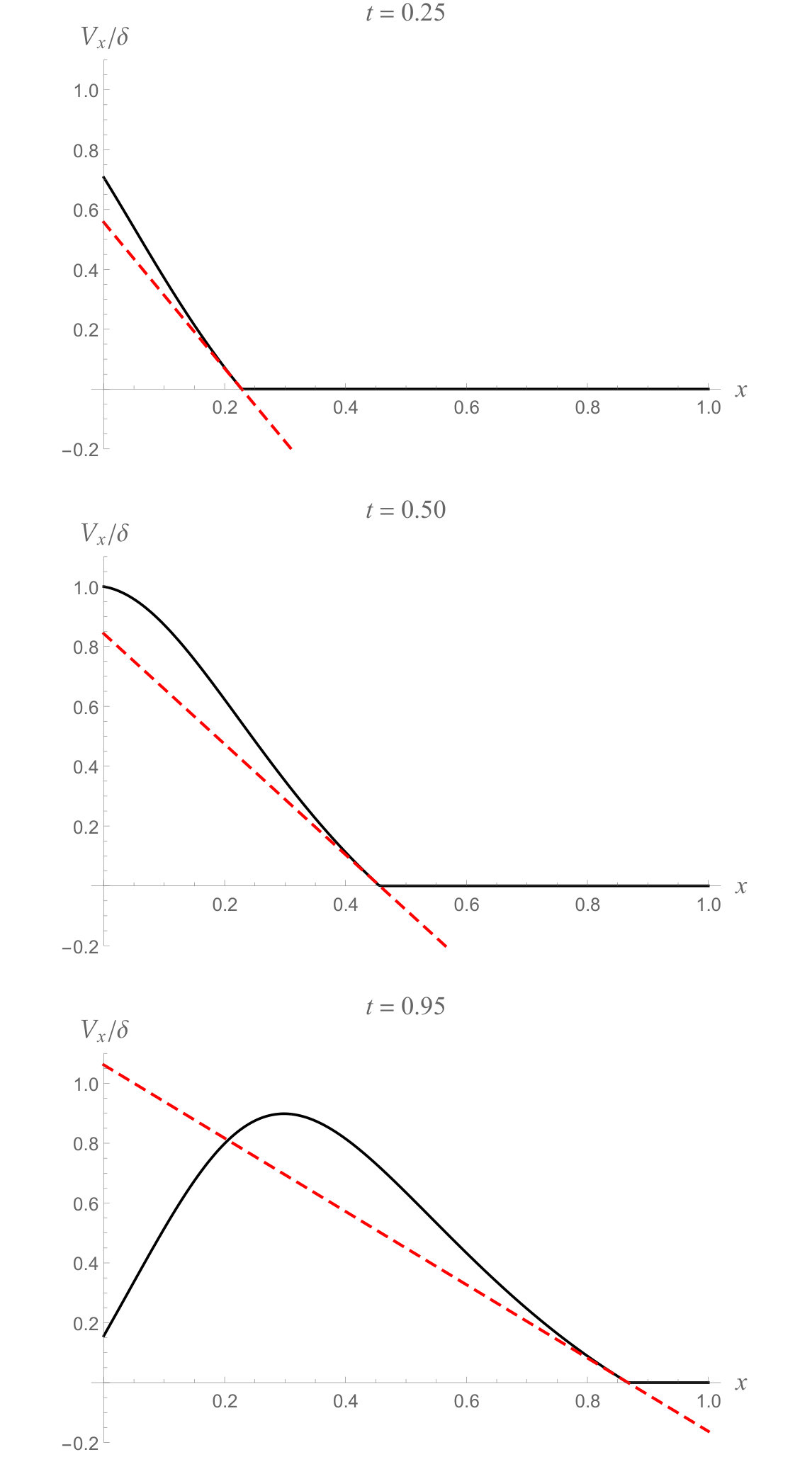 Figure 1
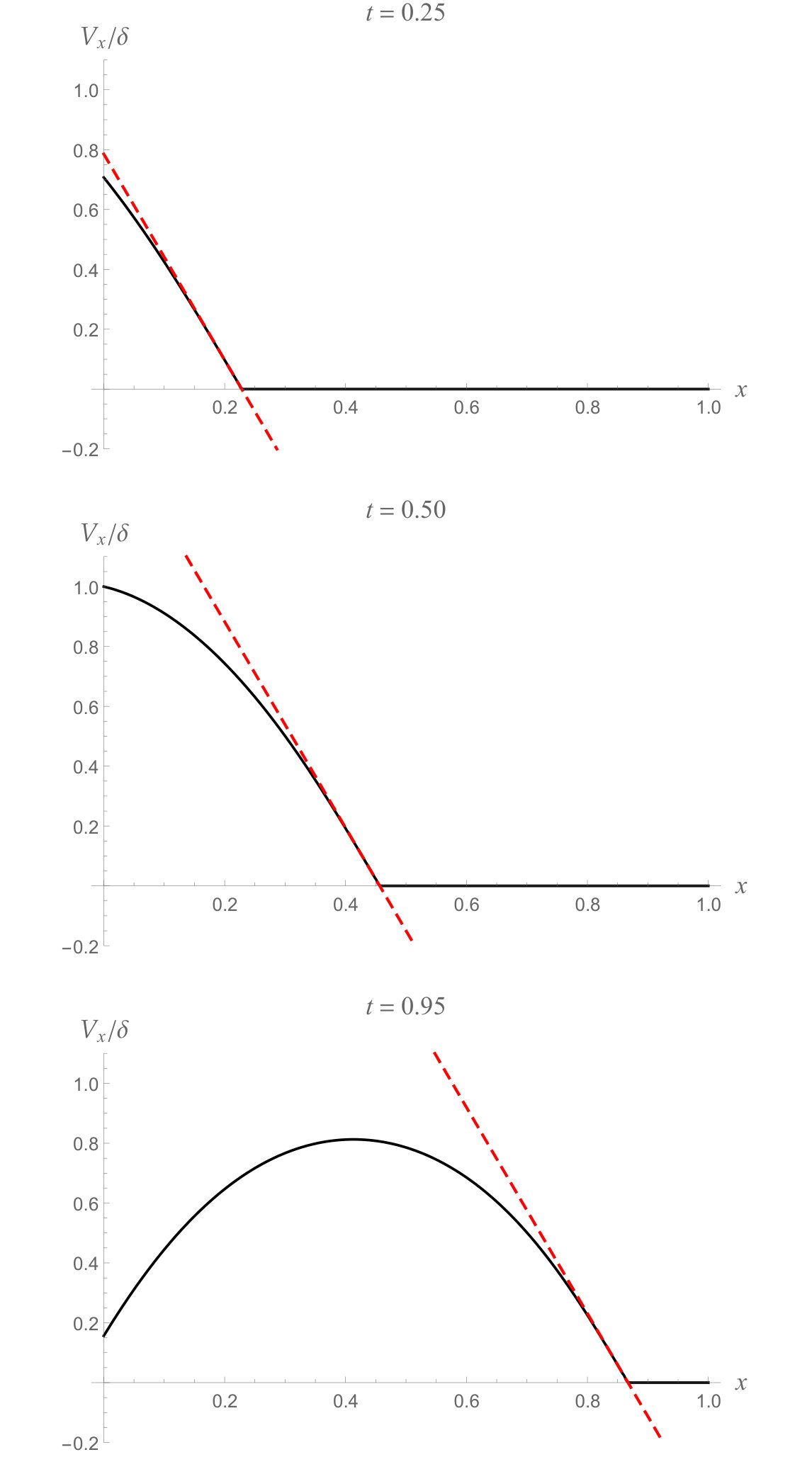 Figure 2
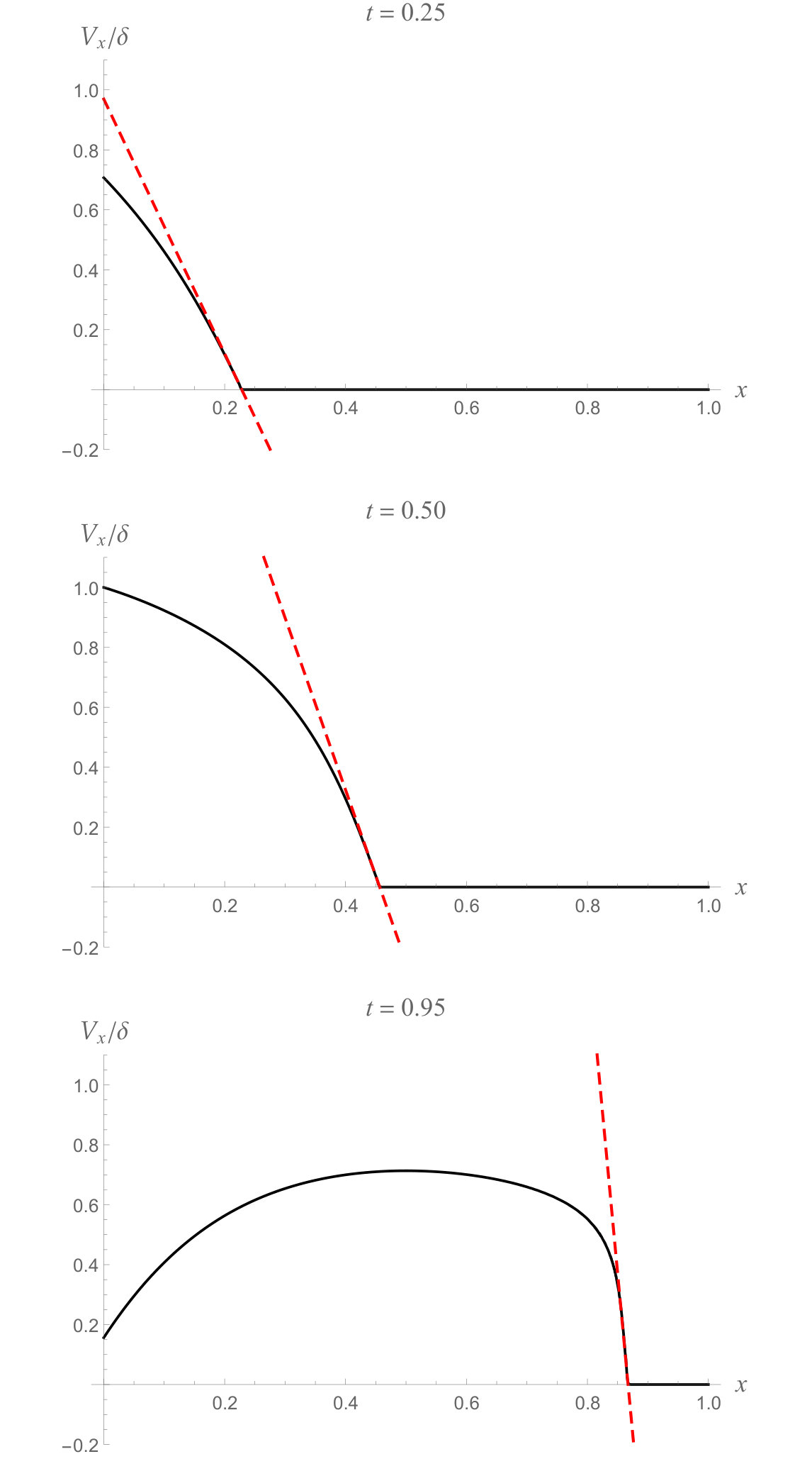 Figure 3
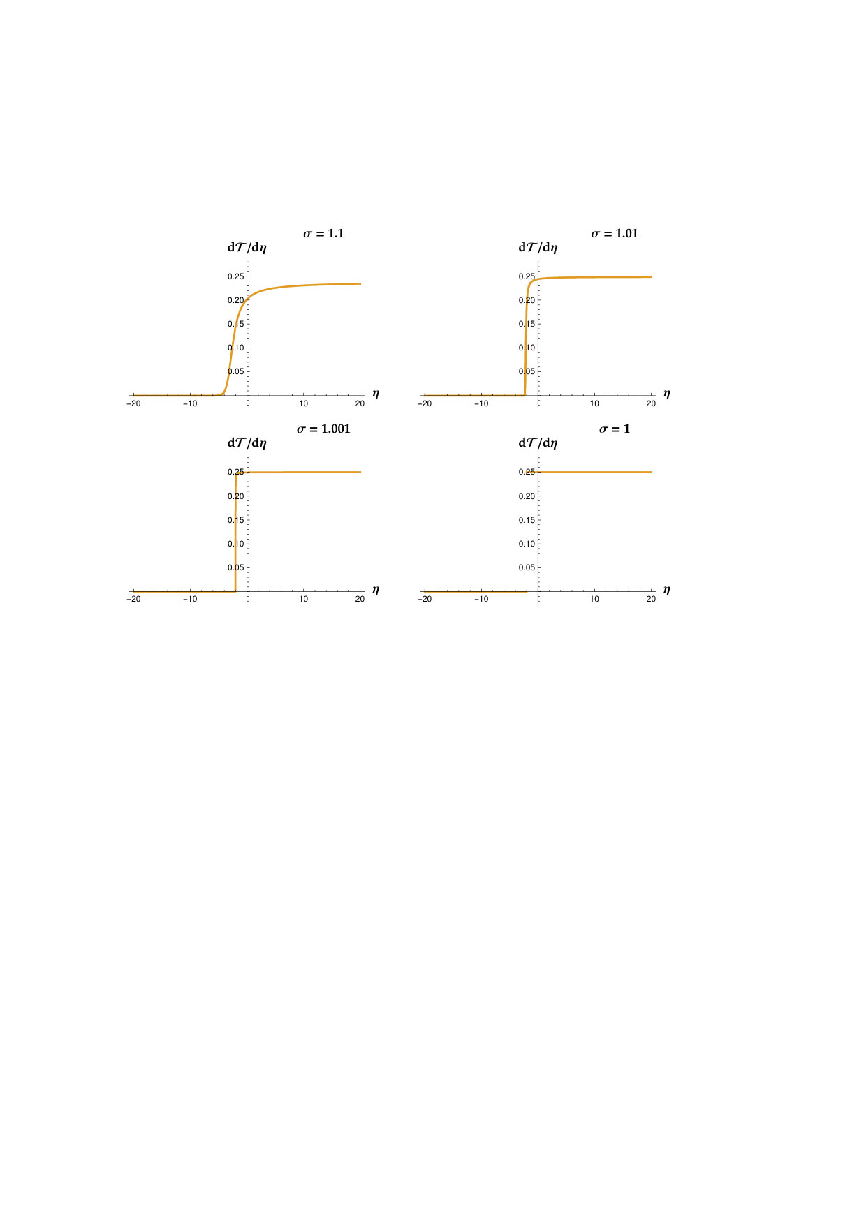 Figure 4
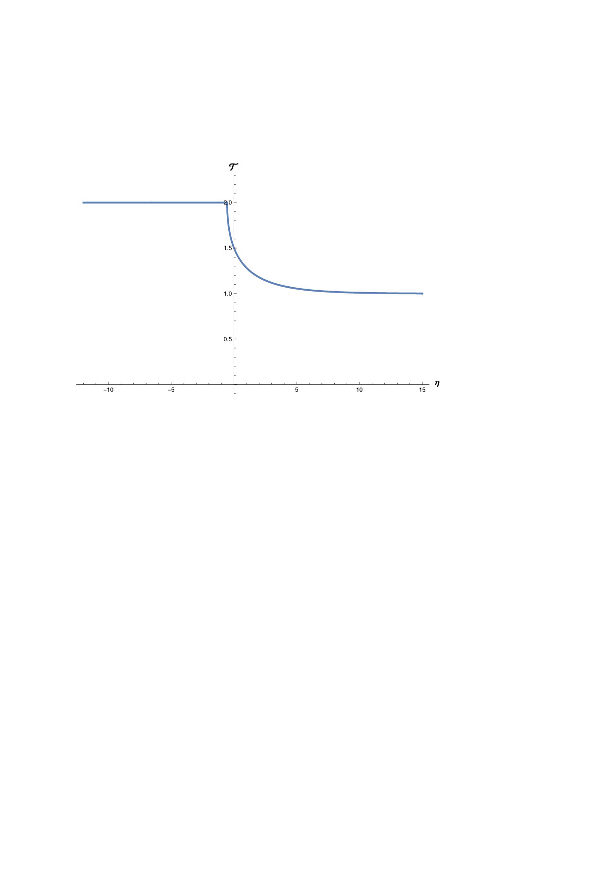 Figure 5
Peer Reviews
No public reviews on file for this paper yet. If you reviewed it on a platform where reviews are public (OpenReview, ICLR, NeurIPS, ICML), you can paste yours below so the community can read it here.
Videos
No videos yet. Explain this paper in a talk, walkthrough, or lecture? Add one.
On the propagation of temperature-rate waves and traveling waves in rigid conductors of the Graffi–Franchi–Straughan type
**Sandra Carillo
Dipartimento di Scienze di Base e Applicate
per l’Ingegneria, Università di Roma La Sapienza ,
Via Antonio Scarpa 16, 00161 Rome, Italy
&
I.N.F.N. - Sezione Roma1, Gr. IV - M.M.N.L.P., Rome, Italy
Pedro M. Jordan111Also at: Acoustics Divivision, U.S. Naval Research Laboratory, Stennis Space Center, Mississippi 39529, USA.
Entropy Reversal Consultants, L.L.C.,
P. O. Box 0691, Abita Springs, LA 70420, USA**
Abstract
We examine second-sound phenomena in a class of rigid, thermally conducting, solids that are described by a special case of the Maxwell–Catteneo flux law. Employing both analytical and numerical methods, we examine both temperature-rate waves and thermal traveling waves in this class of thermal conductor, which have recently been termed Graffi–Franchi–Straughan type conductors. In the present study, the temperature-dependent nature of the thermal relaxation time, which is the distinguishing feature of this class of conductors, gives rise to a variety of nonlinear effects; in particular, finite-time temperature-rate wave blow-up and temperature traveling waveforms which exhibit a “tongue”. The presentation concludes with a discussion of possible follow-on studies.
keyword Graffi–Franchi–Straughan conductors; Maxwell–Cattaneo law; temperature-rate waves; traveling wave solutions; Lambert -function
1 Introduction
Absent the presence of source terms, the most general form of the system that describes the propagation of second-sound (i.e., thermal waves) in the ‘class’ of rigid, homogeneous and isotropic, solids that the present authors have termed Graffi–Franchi–Straughan (GFS) conductors [5] reads
[TABLE]
where denotes the absolute temperature, is the heat flux vector, is the constant-volume specific heat [3], is the thermal conductivity, is a positive constant that carries (SI) units of , and is the (constant) mass density of the conductor. Eq. (1.1a), we observe, is a special case of the Maxwell–Cattaneo (MC) law, i.e., a special case of the flux constitutive relation [11, 18, 19, 23, 24, 28]
[TABLE]
specifically, the former follows from the latter on setting , where
[TABLE]
which is the distinguishing feature of GFS conductors. Here, denotes the relaxation time for phonon processes that are dissipative because they do not conserve phonon momentum [11].
Recalling arguments from an earlier (unpublished) contribution by Graffi, Franchi and Straughan [16], in 1994, used the derivation of Eq. (1.1a) to illustrate a theoretically-motivated means by which the temperature dependence of may arise. In particular, they noted that Eq. (1.1a) identically satisfies the following generalization of the Clausius–Duhem inequality:
[TABLE]
which Franchi and Straughan [16, p. 728] attribute to Graffi; see also Franchi [15] and Straughan [28, §1.2]. As alluded to above, however, GFS conductors must at present be regarded as hypothetical constructs since, to the best of our knowledge, the literature does not contain any examples of actual solids wherein q is described by Eq. (1.1a).
Nevertheless, GFS conductors exhibit a number of interesting mathematical properties that, from our perspective, make them worthy of investigation. For example, the GFS form of plays a critical role in establishing the following:
- •
The empirically based relation for second-sound in rigid solids
[TABLE]
where , , and are fitting parameters, has been shown to be applicable to NaF, for K, and Bi, for K; see, e.g., Refs. [10, 11] and those cited therein. On comparing with Sys. (1.1), it is easily seen that setting , , and reduces Eq. (1.5) to Eq. (1.3). However, the fact that is a constant necessitates the additional requirement const. This is true, as has long been known, in the case of many real solids when , where denotes the Debye temperature of the solid in question; see, e.g., Ref. [3, §2]. From a strictly theoretical standpoint, then, Eq. (1.5) also applies to GFS conductors in the high-temperature regime, i.e., under conditions yielding const.
- •
When is given by Eq. (1.3) and and are both taken to be constant, the flux relation under Morro–Ruggeri (MR) theory [22] reduces to its simplest possible special case that still exhibits explicit dependence on ; i.e., the simplest possible special case in which Ref. [22, Eq. (48)] does not degenerate into a particular case of Eq. (1.2) (above).
- •
When is given by Eq. (1.3), , the generalized expression for the internal energy density under Coleman–Fabrizio–Own (CFO) theory [9] (see also Refs. [10, 11, 22]), reduces to it simplest possible special case that still exhibits explicit dependence on ; i.e., the simplest possible special case in which does not degenerate into the classical expression for the internal energy density of a rigid solid.
The primary aim of this communication is to present numerical simulations of the second-sound phenomena that the present authors examined in Ref. [5] using only analytical methods. In particular, we simulate both temperature-rate waves and traveling waves predicted by the following special case of Sys. (1.1):
[TABLE]
As in Ref. [5], we have assumed , where the constant is the value of the thermal conductivity at some reference temperature; we have taken to be a constant (), but have also made use of the fact that under the rigid solid idealization222For details on the justification/rational behind the use of the approximation when modeling the flow of heat in real solids, see, e.g., Refs. [6, 14, 25]., where denotes the constant-pressure specific heat; and we have confined our attention to one-dimensional (1D) heat flow along the -axis, a propagation geometry which renders and .
To this end, the present article is organized as follows. In Sect. 2, a review of the temperature-rate wave analysis carried out in Ref. [5] is presented. In Sect. 3, numerical simulations of temperature-rate waves are performed and results obtained are compared with our analytical findings. Then, in Sect. 4, a traveling wave analysis of Sys. (1.6) is performed and a two of the resulting solution profiles are studied numerically. And lastly, in Sect. 5, connections to other works are discussed and possible follow-on studies are noted.
2 Temperature-rate waves: Analytical results
2.1 Brief history and related works
By a temperature-rate wave333Also known as a temperature-rate discontinuity wave and a discontinuity (or acceleration) wave; see, e.g., Refs. [21] and [23, §7.4], respectively. we mean a singular surface, i.e., a wavefront, across which the first derivatives of the temperature field suffer a jump discontinuity; see, e.g., Refs. [21, 28]. What makes these waves so interesting is the fact that, under certain conditions, the jump amplitude can exhibit finite-time blow-up, even when the imposed thermal disturbance is continuous. Today, it is generally accepted that temperature-rate wave amplitude blow-up signals the formation of a thermal shock [28], i.e., a propagating surface across which itself suffers a jump.
2.2 Mathematical preliminaries: Characteristic speed
Letting denote the thermal diffusivity [14], we begin this subsection by recasting Sys. (1.6) in (equivalent) matrix form, specifically, as
[TABLE]
The eigenvalues, , of the coefficient matrix satisfy the characteristic equation , where denotes the identity matrix; thus, , where the characteristic speed of second-sound under Sys. (2.1) is
[TABLE]
and the characteristics of Sys. (2.1) are defined by . Since and unequal, it follows that this (quasilinear) system is a strictly hyperbolic [20] one. Therefore, solutions of Sys. (2.1) satisfy the requirements of causality provided is bounded, where from Eq. (2.2) we see that as .
Since is one of the assumptions on which Sys. (1.6) is based, the breakdown of our model as does not pose a difficulty for us. To gain deeper insight into the behavior of , it is instructive to consider finite- and small-amplitude thermal disturbances. Under the weakly-nonlinear and linear approximations Eq. (2.2) becomes
[TABLE]
where in this study denotes the initial temperature of the conductor, and
[TABLE]
respectively. Here, we see that , when , while , when . This, we observe, is the opposite of the behavior exhibited under the (bi-directional) model equations of classical acoustics; see, e.g., Ref. [17, §4()], and note that , the thermodynamic pressure in Ref. [17], corresponds to .
Lastly, to simplify the forthcoming temperature-rate wave analysis, we now introduce the following non-dimensional variables:
[TABLE]
where denotes the conductor’s thickness, and recast Sys. (2.1) in non-dimensional form, viz.:
[TABLE]
where, for convenience, we have set
[TABLE]
all superscript circles have been omitted but should remain understood, and we note for later reference that is the non-dimensional form of .
2.3 Formulation
Now consider a rigid conducting slab, whose (normalized) thickness is unity, wherein the temperature and heat flux are described by Sys. (2.6). We suppose the slab is stationary and that, initially, and the slab is at a uniform temperature (i.e., ) throughout. Beginning at time , let a temperature pulse of the form
[TABLE]
be applied to the boundary , while the boundary is held at temperature . Here, the pulse duration (or width) is a constant; the amplitude function is assumed to be continuously differentiable, nonzero on the interval , and such that but ; and denotes the Heaviside unit step function.
Since Sys. (2.6) is strictly hyperbolic, a planar temperature wavefront , across which , but , begins propagating from the boundary , along the positive -axis, with speed relative to the slab, where we observe that under the present formulation. Here, employing the standard notation of singular surface theory, denotes the amplitude of the jump in the value of the function across , where are assumed to exist, and superscripts correspond to the regions ahead of and behind , respectively. Since, under this formulation, suffers a jump discontinuity across it, the surface is clearly a temperature-rate wave.
2.4 Amplitude evolution
Observing now that is, at most, a function of only , and referring the reader to Refs. [4, 28] for details, it is a straightforward matter to show that , where we have set for convenience and is the location of at , and that the jump in satisfies the Bernoulli equation
[TABLE]
Here, use has been made of
[TABLE]
which is usually referred to as the kinematic condition of compatibility 444See Ref. [28, §4.1] and those cited therein; see also Bland [4, §6.9], who refers to this relation as ‘Hadamard’s lemma’., where , the 1D displacement derivative, gives the time-rate-of-change measured by an observer traveling with ; we have set for convenience; and it should be noted that, since the slab’s initial temperature was assumed to be constant, we took in deriving Eq. (2.9).
Making use of the substitution , Eq. (2.9) is transformed into a linear ODE, which is easily integrated; its exact solution can be expressed as
[TABLE]
where the (negative) constant , known as the critical amplitude, is given by
[TABLE]
According to Eq. (2.11), can evolve in any one of the following four ways:
- (i)
If , then for and from above as . 2. (ii)
If and , then for and from below as . 3. (iii)
If , then for all . 4. (iv)
If and , then for and, moreover, as , where
[TABLE]
2.5 Stability results
While we have obtained the exact solution of Eq. (2.9), it is nevertheless instructive to investigate the steady-state behavior of using qualitative methods; i.e., to examine the stability characteristics of the equilibrium solutions , which of course correspond to the roots of the quadratic equation .
As a phase plane analysis reveals, is always unstable while is always stable. This means that a bifurcation does not occur in the case of Eq. (2.9); i.e., there is no interchange of stability between the two equilibria of this ODE. The instability of also means that the constant solution in Case (iii) is unstable as well; i.e., any discrepancy, however small, in achieving will yield either Case (ii) or (iv).
3 Temperature-rate waves: Numerical results
While interesting and useful, temperature-rate wave results do not provide any information on the behavior of the temperature field behind
Hence, to explore this aspect of the GFS model, and to illustrate the most important findings of Sect. 2.4, we now turn to computational methods. In this section, we present a series of numerical simulations based on the slab initial-boundary value problem (IBVP) formulated in Sect. 2.3, which we now express as:
[TABLE]
Here, so that Sys. (2.6) could be recast as a single PDE, we have introduced
[TABLE]
where . Furthermore, , where is a constant; , where is the time required for to complete its initial transit of the interval (i.e., ); and of course .
In the case of IBVP (3.1) the temperature-rate wave amplitude expression, i.e., Eq. (2.11), becomes
[TABLE]
where the jump was determined using the expression for , the fact that , and the special case of Eq. (2.10), while the expression for the blow-up time, i.e., Eq. (2.13), assumes the form
[TABLE]
Also, it should be noted that the amplitude of the jump in the time derivative of the boundary condition at across the plane is .
Since an exact analytical solution does not appear to be possible, we turn to the calculus of finite differences and introduce the mesh points , where for each and for each . Here, the spatial- and temporal-step sizes are defined as and , respectively, where and are integers and is the right-hand endpoint555Of course, if , then the restriction on becomes . of the temporal interval over which the solution of IBVP (3.1) shall be computed.
With our (1D) mesh established, and guided by the treatment of similar equations presented in Refs. [2, 17], we construct the following simple discretization of Eq. (3.1a):
[TABLE]
where . On setting and then solving for , the most advanced time-step approximation, we obtain the (explicit) finite difference scheme (FDS)
[TABLE]
which holds for each and . In turn, discretization of the boundary conditions gives
[TABLE]
where we note our use of the ghost points666A numerical device that allows us to discretize the Neumann boundary conditions of our problem using centered-difference quotations, i.e., consistent with how the spatial derivatives in Eq. (3.1a) are discretized in our finite difference scheme; see, e.g., Ref. [29]. , while the initial conditions become
[TABLE]
In Figs. 1–3 we have presented temperature profile plots corresponding to Cases (i), (iii), and (iv), respectively. These time-sequence plots depict the evolution of the vs. solution profile under IBVP (3.1), with normalized by , during ’s initial transit of the slab. The curves shown in solid black were produced from data sets computed by a simple algorithm which implemented FDS (3.6) on a desktop computer running Mathematica (ver. 11.2). Interpolations between the points were then accomplished using the cubic interpolation routine that is a built-in part of this software package. The red broken lines, which were generated from Eq. (3.3), have been included to illustrate the behavior of the temperature-rate wave amplitudes; as under IBVP (3.1), the slopes of these lines give the values of , at their points of tangency to the solution profiles, at the indicated times.
For consistency across these three figures, and ease of computation, we have selected the common values (, ) and , , (). It should be noted that of those we tested, with fixed, was the smallest value of for which both FDS (3.6) was numerically stable and we could place, in the case of Fig. 3, very close to, but to the left of, the boundary . The values of and selected were based on a heuristic search to find the smallest such values, subject to , that accurately captured the manifestation of the temperature-rate wave on the temperature profile in the last frame of Fig. 3.
In Fig. 1 we observe, as predicted in Case (i), the slope of the profile at the wavefront decreasing to zero, as , when . In Fig. 2 we see, as predicted in Case (iii), the slope of the profile at the wavefront remaining constant; specifically, . In contrast, Fig. 3777. Note that in Fig. 3, ., which captures approximately of the ‘lifetime’ of , clearly illustrates the exponential increase in as , as predicated in Case (iv). In particular, the last frame of Fig. 3 shows the slope on the leading side of our solution profile becoming nearly vertical at the wavefront, strongly suggesting that a thermal shock is about to form.
4 Traveling wave analysis888The reader
should be aware that the analysis presented in Ref. [5, §3] contains a number of omissions, misstatements, and misprints. In the present section, these issues have, without identification nor comment, all been remedied/corrected.
4.1 Associated ODE, jump magnitude
Assuming right-running waveforms propagating along the -axis, we take the dependence of and on and to be of the form and , where is the wave variable and is the (constant) wave speed. On substituting these ansatzs into Sys. (1.6) we obtain, after simplifying, the system of ODEs
[TABLE]
a (trivial) solution of which, we observe, is
[TABLE]
Here, a prime denotes and is a constant.
Now eliminating between the equations of Sys. (4.1), after integrating Eq. (4.1b) once, and then assuming999That is, we are seeking kink [1], and kink-like, traveling wave solutions. that , as , we obtain the following Abel equation [13] for the temperature field:
[TABLE]
which is the associated ODE of Sys. (1.6). Here, we recall that is the thermal diffusivity; the constant denotes a reference state value of ; and enforcement of the asymptotic condition gives , where is the resulting constant of integration.
An inspection of Eq. (4.3) reveals that , the only equilibrium point of this ODE, is unstable for , but stable for , where
[TABLE]
Here, we observe that is a degenerate case in the following sense: satisfies Eq. (4.3), and it is also true that
[TABLE]
i.e., taking causes to exhibit a jump discontinuity at , the magnitude of which is
[TABLE]
Introducing now the dimensionless temperature and dimensionless wave variable , Eq. (4.3) is reduced to
[TABLE]
Here, is a characteristic length; we have set
[TABLE]
where implies ; and , the dimensionless version of the wave speed , is given by
[TABLE]
where we note that (i.e., is the dimensionless version of ). Also, for later reference we observe that, in terms of the present dimensionless quantities, Eqs. (4.2) and (4.6) become
[TABLE]
where denotes the dimensionless version of and , and
[TABLE]
respectively.
4.2 Complete stability results
A full phase plane analysis of Eq. (4.7) reveals the following:
- (I)
If and , then is unstable (above) and , where as . 2. (II)
If and , then is unstable (below) and . 3. (III)
If and , then , where as . 4. (IV)
If and , then , with as . 5. (V)
If and , then , where as . 6. (VI)
If and , then is stable (above) and . 7. (VII)
If and , then is stable (below) and , with as , respectively.
Here, , where is a (known) positive constant; however, as Cases (I), (IV), and (VI) shall be of particular interest to us, we hereafter limit our attention to .
Returning to Eq. (4.7), we separate variables and integrate; this yields, after then applying and enforcing the condition at ,
[TABLE]
where .
In the next two subsections, the cases of and are treated consecutively.
4.3 The case
For , the integral curves take the form
[TABLE]
where denotes the principal branch of the Lambert - function [12] and we have set . For the case , the solution profile is seen to be a piecewise-linear, but continuous, function of ; it was constructed by joining together, at the point , Eq. (4.10), with , and the special case of Eq. (4.12).
From Eq. (4.13) we find that as . It can, however, be shown that the temperature gradient in this case is bounded; specifically, , for all , where in this subsection the temperature gradient is given by
[TABLE]
From Eq. (4.14) it is clear that corresponds to Case (iii), i.e., the constant amplitude case, of our temperature-rate wave analysis (recall Sect. 2.4). The sequence shown in Fig. 4 depicts the steepening of the temperature gradient profile as (from above); in this limit, the vs. profile tends to a step function, i.e., a temperature-rate wave in the present setting, of (jump) magnitude .
4.4 The case
On joining, at the point (see below), the special case of Eq. (4.12) to the constant-temperature solution given in Eq. (4.10), the piecewise-defined integral curve corresponding to this range of -values is readily constructed, viz.:
[TABLE]
Here, we note the restriction and observe that the value of on the interval follows on setting in Eq. (4.10). Also, is given by
[TABLE]
where Eq. (4.16) was obtained by setting the argument of (in Eq. (4.15)) equal to and then solving for , where is a branch point of the -function; again, see Ref. [12].
Along with the fact that Eq. (4.15) describes a bounded, continuous, waveform, for which is a stable equilibrium, Fig. 5 also reveals that for , the GFS traveling wave profile exhibits what Zel’dovich and Raizer [31, Fig. 10.3b] refer to as a (preheating) ‘tongue’.
5 Closure
From the mathematical standpoint, the present analysis has shown that the qualitative behavior of Sys. (1.6) is very much like that exhibited by the 1D version of the ‘Darcy–Jordan’ model101010Also known as the ‘Jordan–Darcy’ model; see, e.g., Ref. [26] and those cited therein. [17] (of poroacoustics) when the fluid phase consists of a retrograde fluid111111Fluids that exhibit rarefaction (or ‘negative’) shocks; see, e.g., Ref. [30] and those cited therein. Note also that retrograde fluids correspond to in Ref. [17], wherein denotes the coefficient of nonlinearity.. This analogy is most evident in the case of temperature-rate waves; recall the behavior of (see Sect. 2.2), and observe that corresponds to , where is used in Ref. [17, §4] to denote the dimensionless over pressure in a regular fluid.
It is also noteworthy that the behavior of the waveforms observed in Sect. 4 under the and cases corresponds to taking and , respectively, in Christov and Jordan [8, pp. 1126–1128], who examined traveling waves under the MC law with a linear function of and const.
With regard to possible follow-on studies, the obvious next step from the numerical standpoint is to examine thermal shock phenomena under Sys. (1.6) using what are known as ‘shock capturing’ schemes (see, e.g., Ref. [8] and those cited therein), which are more elaborate than the simple explicit scheme we employed in Sect. 3. From the analytical standpoint, extensions of the present study might include performing the above analyzes on the GFS special cases of MR theory and CFO theory; recall the second and third bulleted items in Sect. 1.
On the other hand, Sys. (1.1) could be recast in terms of what Straughan [27] has termed ‘Cattaneo–Christov’ theory. Under this generalization of the MC law, which Christov [7] proposed in 2009, the simple partial time derivative that acts on would be replaced by a Lie derivative—one corresponding to Oldroyd’s upper convected derivative—which would then make Sys. (1.1) applicable to moving (GFS) conductors; to this latter point, see also the first footnote in Ref. [9, p. 136].
Acknowledgments
The authors are grateful to the anonymous referee for his/her helpful comments and for bringing Ref. [10] to their attention. S.C. thanks the financial support of G.N.F.M.–I.N.d.A.M., I.N.F.N. and Università di Roma La Sapienza, Rome, Italy.
The reference list from the paper itself. Each links out to its DOI / PubMed record.
- 1[1] J. Angulo, Nonlinear Dispersive Equations: Existence and Stability of Solitary and Periodic Travelling Wave Solutions, in: Mathematical Surveys and Monographs, vol. 156, American Mathematical Society, 2009.
- 2[2] S. Bargmann, P. Steinmann, P.M. Jordan, On the propagation of second-sound in linear and nonlinear media: Results from Green–Naghdi theory, Phys. Lett. A 372 (2008) 4418–4424.
- 3[3] M. Blackman, The specific heat of solids, in: S. Flügge (Ed.), Handbuch der Physik, vol. VII/1, pp. 325–382, Springer, 1955.
- 4[4] D.R. Bland, Wave Theory and Applications, Oxford University Press, 1988.
- 5[5] S. Carillo, P.M. Jordan, Second-sound in nonlinear Graffi–Franchi–Straughan type one dimensional heat conductors, in: M. Ciarletta, et al. (Eds.), Proceedings of the 11th International Congress on Thermal Stresses, Salerno, Italy (5–9 June 2016), pp. 35–38.
- 6[6] H.S. Carslaw, J.C. Jaeger, Conduction of Heat in Solids, 2nd edn., Oxford University Press, 1959, §1.6.
- 7[7] C.I. Christov, On frame indifferent formulation of the Maxwell–Cattaneo model of finite-speed heat conduction, Mech. Res. Commun. 36 (2009) 481–486.
- 8[8] I.C. Christov, P. M. Jordan, On the propagation of second-sound in nonlinear media: Shock, acceleration and traveling wave results, J. Thermal Stresses 33 (2010) 1109–1135.