Degree-d-invariant laminations
William P. Thurston, Hyungryul Baik, Yan Gao, John H. Hubbard, Tan, Lei, Kathryn A. Lindsey, Dylan P. Thurston

TL;DR
This paper explores degree-d-invariant laminations as models for polynomial dynamics, introduces primitive majors as a parameterization tool, and presents a combinatorial method for computing core entropy without Hubbard trees.
Contribution
It introduces primitive majors as a new combinatorial framework and provides a direct method to compute core entropy for degree-d polynomials.
Findings
Primitive majors form a spine for polynomial parameter spaces.
A combinatorial approach allows core entropy calculation without Hubbard trees.
The framework models polynomial dynamics via invariant laminations.
Abstract
Degree--invariant laminations of the disk model the dynamical action of a degree- polynomial; such a lamination defines an equivalence relation on that corresponds to dynamical rays of an associated polynomial landing at the same multi-accessible points in the Julia set. Primitive majors are certain subsets of degree--invariant laminations consisting of critical leaves and gaps. The space of primitive degree- majors is a spine for the set of monic degree- polynomials with distinct roots and serves as a parameterization of a subset of the boundary of the connectedness locus for degree- polynomials. The core entropy of a postcritically finite polynomial is the topological entropy of the action of the polynomial on the associated Hubbard tree. Core entropy may be computed directly, bypassing the Hubbard tree, using a combinatorial analogue of the…
Click any figure to enlarge with its caption.
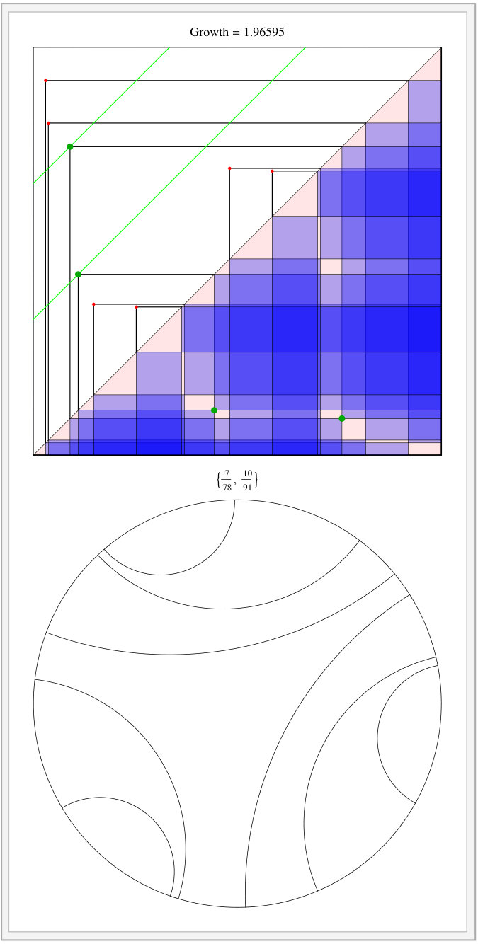 Figure 1
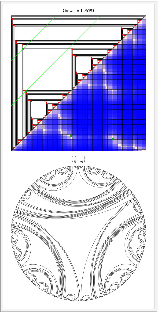 Figure 2
 Figure 3
 Figure 4
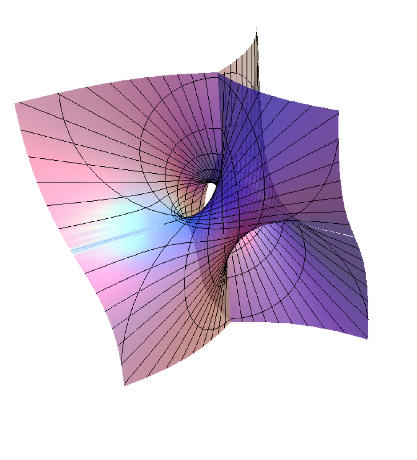 Figure 5
 Figure 6
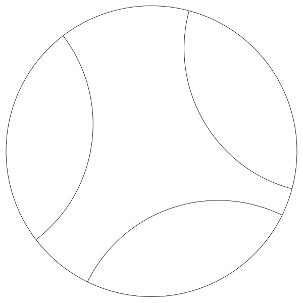 Figure 7
 Figure 8
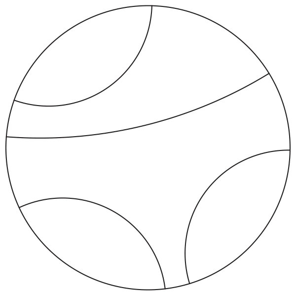 Figure 9
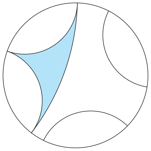 Figure 10
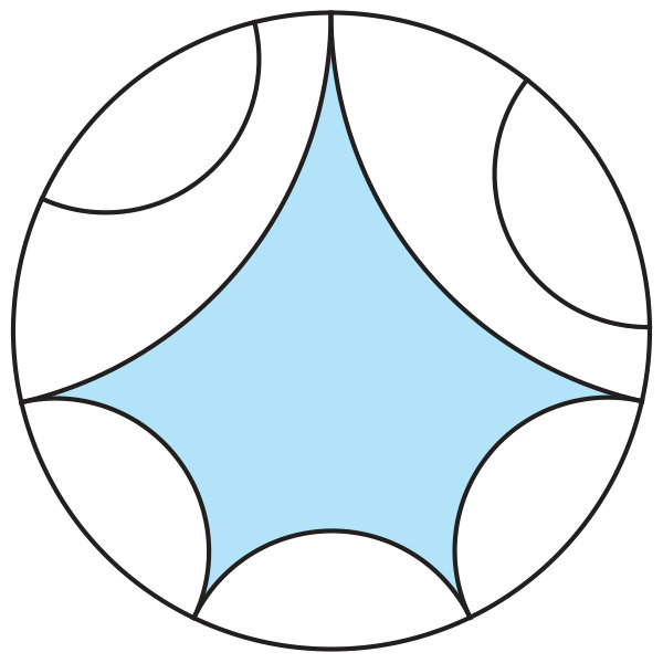 Figure 11
 Figure 12
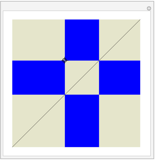 Figure 13
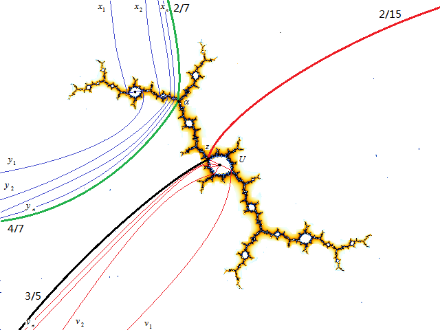 Figure 14
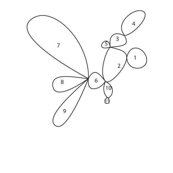 Figure 15
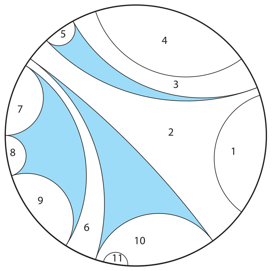 Figure 16
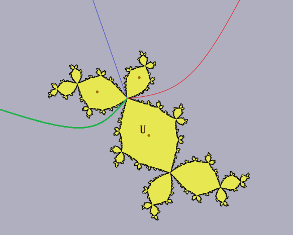 Figure 17
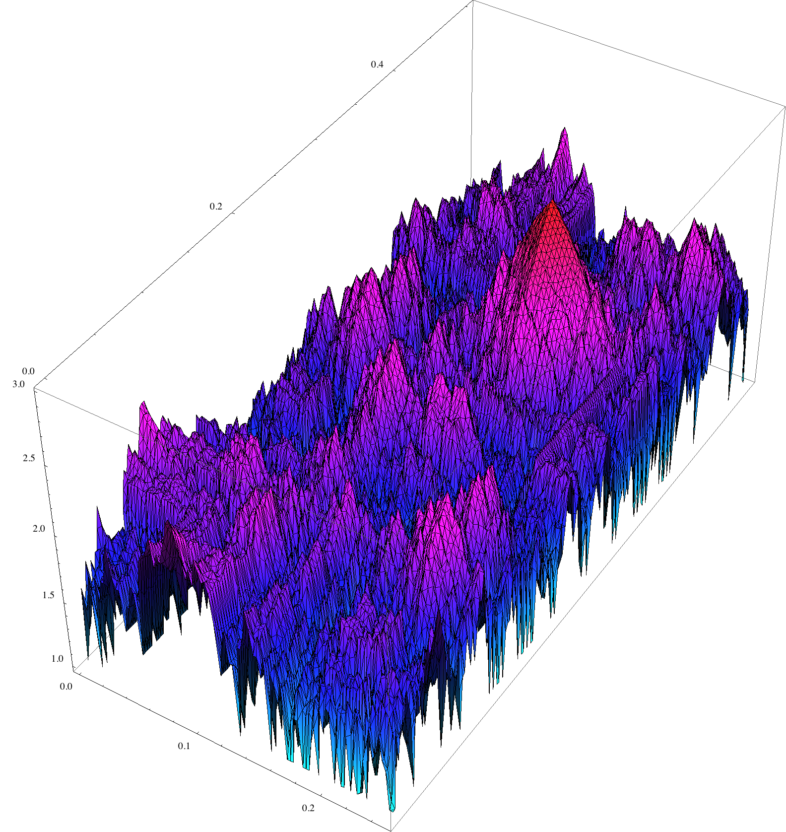 Figure 18
 Figure 19
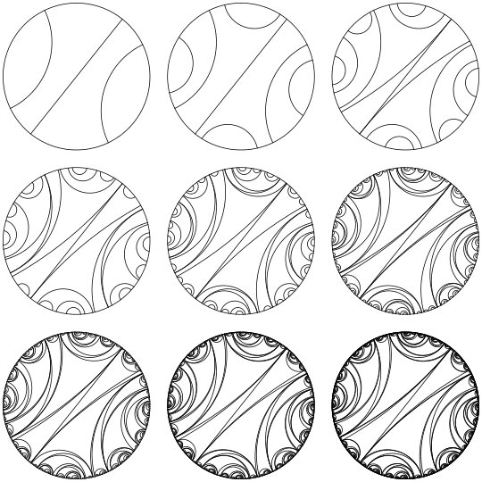 Figure 20
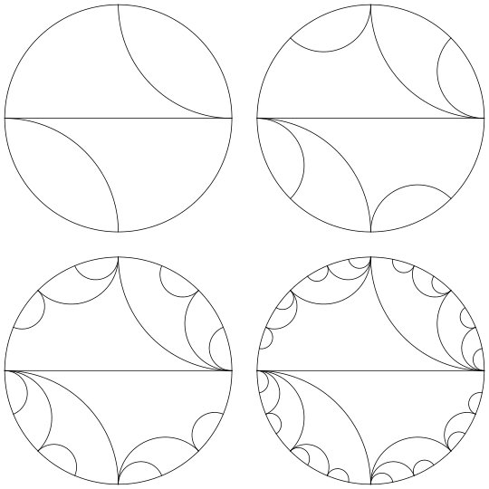 Figure 21
 Figure 22
 Figure 23
 Figure 24
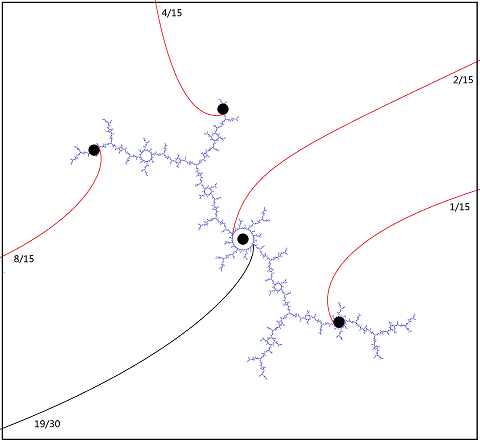 Figure 25
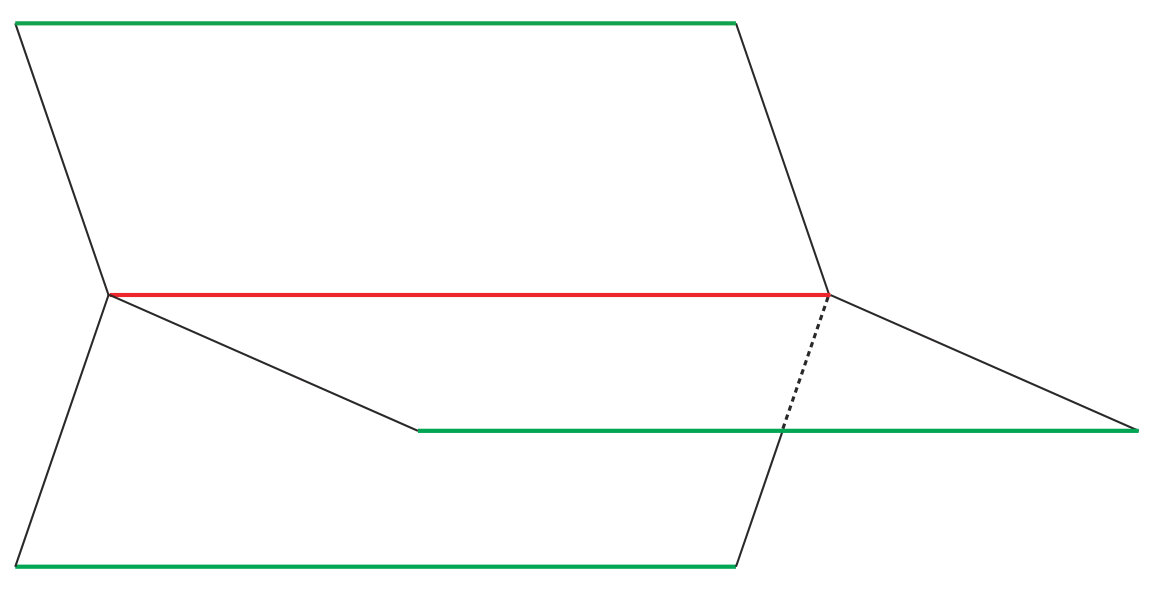 Figure 26
 Figure 27
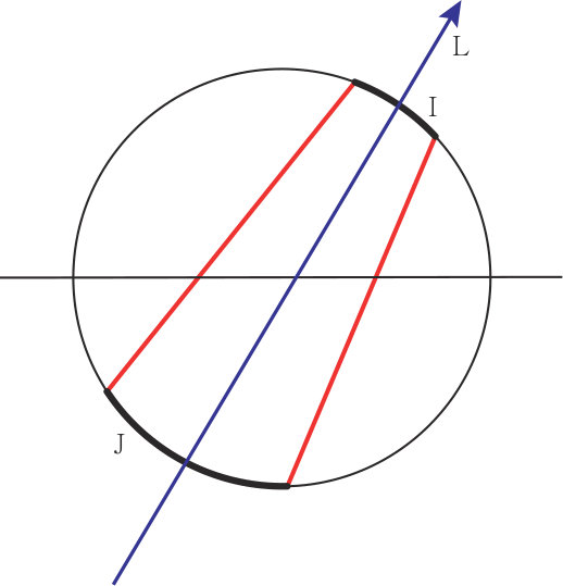 Figure 28
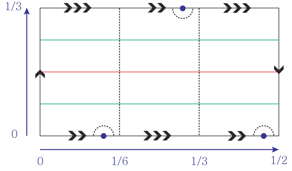 Figure 29
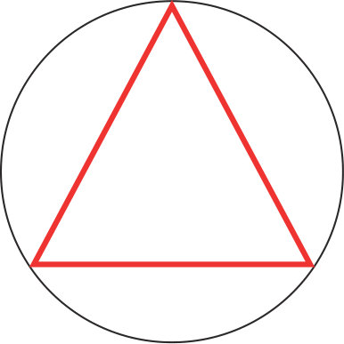 Figure 30
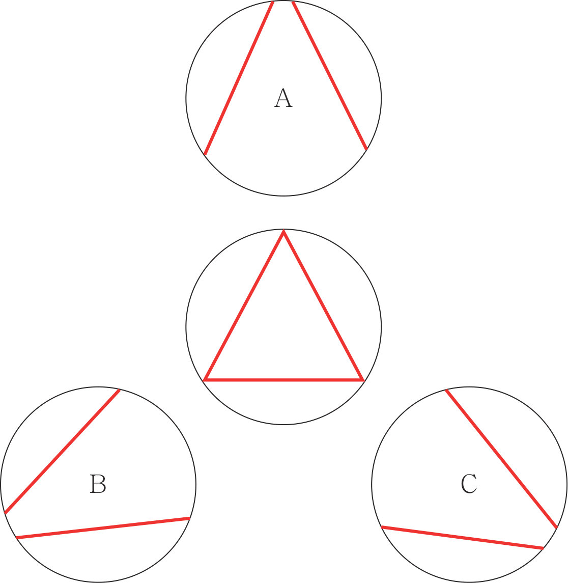 Figure 31
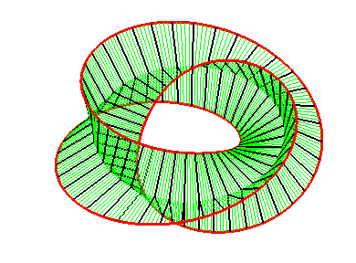 Figure 32
Peer Reviews
No public reviews on file for this paper yet. If you reviewed it on a platform where reviews are public (OpenReview, ICLR, NeurIPS, ICML), you can paste yours below so the community can read it here.
Videos
No videos yet. Explain this paper in a talk, walkthrough, or lecture? Add one.
Taxonomy
TopicsMathematical Dynamics and Fractals · Liquid Crystal Research Advancements · Quantum chaos and dynamical systems
Degree--invariant laminations
William P. Thurston
Department of Mathematics, Cornell University
Ithaca, NY, 14853, USA, and
King Abdulaziz University
Jeddah 22254, Saudi Arabia
,
Hyungryul Baik
Department of Mathematical Sciences, KAIST
291 Daehak-ro Yuseong-gu, Daejeon, 34141, South Korea
,
Gao Yan
Department of Mathematics, Sichuan University, Chengdu, 610065, China
,
John H. Hubbard
Department of Mathematics, Cornell University
Ithaca, NY 14853, USA
,
Tan Lei
Université d’Angers, Faculté des sciences, LAREMA
49045 Angers cedex 01, France
,
Kathryn A. Lindsey
Department of Mathematics, University of Chicago
Chicago, IL 60637, USA
and
Dylan P. Thurston
Department of Mathematics, Indiana University–Bloomington
Bloomington, IN 47405, USA
Abstract.
Degree--invariant laminations of the disk model the dynamical action of a degree- polynomial; such a lamination defines an equivalence relation on that corresponds to dynamical rays of an associated polynomial landing at the same multi-accessible points in the Julia set. Primitive majors are certain subsets of degree--invariant laminations consisting of critical leaves and gaps. The space of primitive degree- majors is a spine for the set of monic degree- polynomials with distinct roots and serves as a parameterization of a subset of the boundary of the connectedness locus for degree- polynomials. The core entropy of a postcritically finite polynomial is the topological entropy of the action of the polynomial on the associated Hubbard tree. Core entropy may be computed directly, bypassing the Hubbard tree, using a combinatorial analogue of the Hubbard tree within the context of degree--invariant laminations.
Preface
During the last year of his life, William P. Thurston developed a theory of degree--invariant laminations, a tool that he hoped would lead to what he called “a qualitative picture of [the dynamics of] degree polynomials.” Thurston discussed his research on this topic in his seminar at Cornell University and was in the process of writing an article on this topic, but he passed away before completing the manuscript. Part I of this document consists of Thurston’s unfinished manuscript. As it stands, the manuscript is beautifully written and contains a lot of his new ideas. However, he discussed ideas that are not in the unfinished manuscript and some details are missing. Part II consists of supplementary material written by the other authors based on what they learned from him throughout his seminar and email exchanges with him. Tan Lei also passed away during the preparation of Part II. William Thurston’s vision was far beyond what we could write here, but, hopefully, this paper will serve as a starting point for future researchers.
Each semester since moving to Cornell University in 2003, William Thurston taught a seminar course titled “Topics in Topology,” which was familiarly (and perhaps more accurately) referred to by participants as “Thurston seminar.” On the first day of each semester, Thurston asked the audience what mathematical topics they would like to hear about, and he tailored the direction of the seminar according to the interests of the participants. Although the course was nominally a seminar in topology, he discussed other topics as well, including combinatorics, mathematical logic, and complex dynamics. Between 2010 and 2012, a high percentage of the seminar participants were dynamicists, and so (with the exception of one semester) Thurston’s seminar during this period primarily focused on topics in complex dynamics. He discussed his topological characterization of rational maps on the Riemann sphere, as well as how to understand complex polynomials via topological entropy and laminations on the circle. During this time, Thurston developed many beautiful ideas, motivated in part by discussions with people in his seminar and in part by email exchanges with others who were at a distance.
His seminar was not an organized lecture series; it was much more than that. He talked about ideas that he was developing at that very moment, as opposed to previously known findings. Thurston invited members of the seminar to be actively involved in the exploration. He often demonstrated computer experiments in class, and he encouraged seminar participants to experiment with his codes. Seminar participants frequently received drafts of Thurston’s manuscript as his thinking evolved. Those fortunate enough to learn from Thurston observed how his understanding of the subject gradually transformed into a beautiful theory.
Part I
Degree--invariant laminations
William P. Thurston
February 22, 2012
1. Introduction
Despite years of strong effort by an impressive group of insightful and hardworking mathematicians and many advances, our overall understanding and global picture of the dynamics of degree rational maps and even degree complex polynomials has remained sketchy and unsatisfying.
The purpose of this paper is to develop at least a sketch for a skeletal qualitative picture of degree polynomials. There are good theorems characterizing and describing examples individually or in small-dimensional families, but that is not our focus. We hope instead to contribute toward developing and clarifying the global picture of the connectedness locus for degree polynomials, that is, the higher-dimensional analogues of the Mandelbrot set.
To do this, the main tool will be the theory of degree--invariant laminations.
We hope that by developing a better picture for degree polynomials, we will develop insights that will carry on to better understand degree rational maps, whose global description is even more of a mystery.
2. Some definitions and basic properties
A degree polynomial map always “looks like” near . More precisely, it is known that is conjugate to in some neighborhood of .
We may as well specialize to monic polynomials such that the center of mass of the roots is at the origin (so that the coefficient of is [math]), since any polynomial can be conjugated into that form. In that case, we can choose the conjugating map to converge to the identity near ; this uniquely determines the map. As Douady and Hubbard noted, we can use the dynamics to extend the conjugacy near inward toward [math] step by step. If the Julia set is connected, we obtain in this way a Riemann mapping of the complement of the Julia set to the complement of the closed unit disk in that conjugates the dynamics outside the Julia set (which is the attracting basin of ) to the standard form .
It has been known since the time of Fatou and Julia (and easy to show) that the Julia set is the boundary of the attracting basin of . We want to investigate the topology of the Julia set, and how this topology varies among polynomial maps of degree . As long as the Julia set is locally connected, the Julia set is the continuous image of the unit circle that is the boundary of the Riemann map around ; the key question is to understand the identifications on the circle made by these maps, and the way the identifications vary as the polynomial varies.
Define a treelike equivalence relation on the unit circle to be a closed equivalence relation such that for any two distinct equivalence classes, their convex hulls in the unit disk are disjoint. (A relation on a topological space is closed if it is a closed subset of .) The condition that the convex hulls of equivalence classes be disjoint comes from the topology of the plane: it translates into the condition that if we take the complement of the open unit disk and make the given identifications on the circle, two simple closed curves that cross the circle quotient using different equivalence classes cannot have intersection number , otherwise the quotient space would not embed in the plane.
To develop a geometric understanding of the possible equivalence relations, it helps to translate the concept into the language of laminations. Given a treelike equivalence relation , there is an associated lamination of the open disk, where the leaves of consist of boundaries of convex hulls of equivalence classes intersected with the open disk. The regions bounded by leaves are called gaps. Some of the gaps of are collapsed gaps, which touch the circle in a single equivalence class, while other gaps are intact gaps. An intact gap necessarily touches the circle in an uncountable set, and its boundary mod is homeomorphic to a circle.
Conversely, given a lamination there is an equivalence relation , usually obtained by taking the transitive closure of the relation that equates endpoints of leaves. However, this relation may not be topologically closed. One can take the closure, which may not be an equivalence relation. It is possible to alternate the operations of transitive closure and topological closure by transfinite induction until it stabilizes to a closed equivalence relation , or simply define as the intersection of all closed equivalence relations that identify endpoints of leaves of .
Often, but not always, the operations and are inverse to each other. If has equivalence classes that are Cantor sets, then will collapse these only to a circle, not to a point. If has chains of leaves with common endpoints, then any leaves in the interior of the convex hull of the chain of vertices will disappear, and new edges may also appear.
A circular order on a set intuitively means an embedding of the set on a circle, up to orientation-preserving homeomorphism. In combinatorial terms, a circular order can be given by a function from triples of elements to the set (interpreted as giving the sign of the area of the triangle formed by three elements in the plane) such that if and only if the elements are not distinct, and is a 2-cocycle, meaning for any four elements , , and , the sum of the values for the boundary of a 3-simplex labeled with these elements is 0. (This implies, in particular, that , etc.) With this definition, it can be shown that any countable circularly ordered set can be embedded in the circle in such a way that is the sign of the area of the triangle formed by the images of , and . One way to prove this assertion is to first observe that a circular order can be ‘cut’ at a point to into a linear order, defined by . It is reasonably well-known that a countable linear order on a set is induced by an embedding of that set in the interval, from which it follows that a circular ordering is induced by an embedding in .
An interval of a circularly-ordered set is a subset with a linear order (=total order) satisfying the condition that
- i.
For , , and
- ii.
For any and any , if then .
Usually the linear order is determined by the subset, but there is an exception if the subset is the entire circularly ordered set. In that case the definition is like cutting a circle somewhere to form an interval. Just as for linear orders, any two elements in a circularly ordered set determine a closed interval , as well as an open interval , etc.
The degree of a map between two circularly ordered sets is the minimum size of a partition of into intervals such that on each interval, the circular order is preserved. If there is no such finite partition, the degree is .
A treelike equivalence relation is degree--invariant if
- i.
If then , and
- ii.
For any equivalence class , the total degree of the restrictions of to the equivalence classes on the set is .
Similarly, a lamination is degree--invariant if
- i.
If there is a leaf with endpoints and , then either or there is a leaf with endpoints and
- ii.
If there is a leaf with endpoints and , there is a set of disjoint leaves with one endpoint in and the other endpoint in .
These conditions on leaves imply related conditions for gaps, from the behavior of the boundary of the gap. In particular, an equivalence relation is degree--invariant if and only if is degree--invariant. As customary, we will use the word ‘quadratic’ as a synonym for degree 2, ‘cubic’ for degree 3, ‘quartic’ for degree 4, etc.
It is worth pointing out that the map is centralized by a dihedral group of symmetries of order , generated by reflection together with rotation where is a primitive th root of unity. Therefore, the set of all degree--invariant laminations and the set of all degree--invariant relations has the same symmetry group.
If is a degree--invariant equivalence relation, a critical class is an equivalence class that maps with degree greater than 1. Similarly, a critical gap in is a gap whose intersection with the circle is mapped with degree greater than 1. The criticality of a class or a gap is its degree minus 1. A critical class may correspond to either a critical leaf, which must have criticality 1, or a critical gap. A critical gap may be a collapsed gap that corresponds to a critical class, or an intact gap.
Proposition 2.1**.**
For any degree--invariant equivalence relation , the total criticality of equivalence classes of together with intact critical gaps of (i.e the sum of the criticality of the critical classes and the intact critical gaps) equals .
Proof.
First, let’s establish that if there is at least one critical leaf or critical gap. We can do this by extending the map to the disk: first extend linearly on each edge of the lamination, then foliate each gap by vertical lines and extend linearly to each of the leaves of this foliation. If there were neither collapsing leaves nor collapsing gaps, this would be a homeomorphism on each leaf and on each gap, so the map would be a covering map, impossible since the disk is simply-connected.
Now consider any critical leaf , the circle with and identified is the union of two circles mapping with total degrees and where . Proceed by induction: if the total criticality in these two circles is and , then the total criticality in the whole circle is .
Now consider any critical gap . Let be the union of with the boundary of , and be its image under , extended linearly on each edge. Any leaf in the image of the boundary of has preimages, from which it follows readily that the total criticality of the map on the complementary regions of is . ∎
Definition 2.2**.**
The major of a degree--invariant lamination is the set of critical leaves and critical gaps. The major of a degree--invariant equivalence relation is the set of equivalence classes corresponding to critical leaves and critical gaps of .
3. Majors
What are the possibilities for the major of a degree--invariant lamination?
We’ll say that the major of a lamination is primitive if each critical gap is a polygon whose vertices are all identified by . We will see later that any degree--invariant lamination is contained in a degree--invariant lamination whose major is primitive; there are sometimes several possible invariant enlargements, and sometimes uncountably many. The invariant enlargements might not come from invariant equivalence relations, but they are useful nonetheless for understanding the global structure of invariant laminations, invariant equivalence relations, and Julia sets for degree polynomials.
Even without a predefined lamination, we can define a primitive degree- major to be a collection of disjoint leaves and polygons each of whose vertices are identified under , with total criticality . In Section 4 we will show how to construct a degree--invariant lamination whose major is the given major. First though, we will analyze the set of all primitive degree- majors.
An element determines a quotient graph obtained by identifying each equivalence class to a point. The path-metric of defines a path-metric on . In addition, has the structure of a planar graph, that is, an embedding in the plane well-defined up to isotopy, obtained by shrinking each leaf and each ideal polygon of the lamination to a point. These graphs have the property that has rank , and every cycle has length a multiple of . Every edge must be accessible from the infinite component of the complement, so the metric and the planar embedding together with the starting point, that is, the image of , is enough to define the major.
The metric on the circle induced by the path-metric on determines a metric on , define as the sup difference of metrics,
[TABLE]
In particular, there is a well-defined topology on .
There is a recursive method one can use to construct and analyze primitive degree- majors, as follows. Consider any isolated leaf of a major . The endpoints of split the circle into two intervals, of length and of length , for some integer . If we identify the endpoints of and make an affine reparametrization to stretch it by a factor of so it fits around the unit circle and place the identified endpoints at 0, the leaves of with endpoints in become a primitive degree major. Similarly, we get a primitive degree major from . If is any ideal -gon of an element , we similarly can derive a sequence of primitive majors whose total degree is .
Theorem 3.1**.**
The space can be embedded in the space of monic degree polynomials as a spine for the set of polynomials with distinct roots, that is, the complement of the discriminant locus. The spine (image of the embedding) consists of monic polynomials whose critical values are all on the unit circle and such that the center of mass of the roots is at the origin.
A spine is a lower-dimensional subset of a manifold such that the manifold deformation-retracts to the spine.
Proof.
We’ll start by defining a map from the space of polynomials with distinct zeroes to . Given a polynomial , we look at the gradient vector field for , or better, the gradient of the smooth function . Any simple critical point for is a saddle point for this flow. Near infinity, the flow lines align very closely to the flow lines for the gradient of , so each flow line that doesn’t tend toward a critical point goes to infinity with some asymptotic argument (angle). Define a lamination whose leaves join the pairs of outgoing separatrices for the critical points. If there are critical points of higher multiplicity or if the unstable manifolds from some critical points coincide with stable manifolds for others (separatrices collide), then define an equivalence relation that decrees that for any flow-line, if the limit of asymptotic angles on the left is not the same as the limit of asymptotic angles on the right, then the two limits are equivalent. For each such equivalence class, adjoin the ideal polygon that is the boundary of its convex hull.
We claim that the lamination so defined is a primitive degree- major. To see that, notice that the level sets of are mapped under to concentric circles, so the flow lines for the gradient flow map to the perpendicular rays emanating from the origin. Each equivalence class coming from discontinuities in the asymptotic angles therefore maps to a single point, since there are no critical points for the image foliation except at the origin in the range of . The total criticality is since the degree of is .
There are many different polynomials that give any particular major. In the first place, note that for any polynomial, if we translate in the domain by any constant (which amounts to translating all the roots in some direction, keeping the vectors between them constant), the asymptotic angles of the upward flow lines from the critical points do not change, so then lamination does not change. We may as well keep the roots centered at the origin. Algebraically, this is equivalent to saying that the critical points are centered at the origin (by considering the derivative of the defining polynomial).
You can think of the spine this way. In the domain of , cut along each upward separatrix of each critical point. This cuts into pieces, each containing one root of (that you arrive at by flowing downhill; whenever there is a path from to whose downhill flows don’t ever meet a critical point, they end up at the same root). For any region, if you glue the two sides of each edge together, starting at the lowest critical point and matching points with equal values for , you obtain a copy of which is really just a copy of the image plane; the seams have joined together to become rays.
You can construct other polynomials associated with the same major by varying the length of the cuts. (These cuts are classical branch cuts). Assuming for now that we are in the generic case with no critical gaps, for each leaf choose a positive real number. Take one copy of for each region of the complement of the lamination, and for each leaf on its boundary, make a slit on the ray at angle from to the point . Now glue the slit copies of together so as to be compatible with the parametrization by . (This is equivalent to forming a branched cover of , branched over the various critical values, with given combinatorial information or Hurwitz data describing the branching.) By uniformization theory, the Riemann surface obtained by gluing the copies of together is analytically equivalent to , and the induced map is a polynomial.
In the nongeneric case (in which there are critical gaps), the set of possibilites branches: it is not parametrized by a product of Euclidean spaces, because of the different possibilities for the combinatorics of saddle connections. Let’s look more closely at the possible structure of saddle connections for the gradient flow of . A small regular neighborhood of the union of the upward separatrices for the critical points has boundary consisting of lines (here is the multiplicity of the critical point); these map to the leaves of the boundary of the corresponding gap of the major. The union of upward separatrices is a tree whose leaves are the vertices of the gap polygon. The height function has the property that induces a function with exactly one local minimum on each boundary component of the regular neighborhood projected to the graph.
We can bypass the enumeration of all such structures by observing that there is a direct way to define a retraction to the case when all critical values equal 1. We think of the graph as a metric graph where the height function has speed 1. Multiply the height function on the compact edges of the graph by while adding the constant times to the height function on each unbounded component that makes it continuous at the vertices. When , the compact edges all collapse, only the unbounded edges remain, and the polygonal gap contains a single multiple critical point with critical value 1.
∎
Corollary 3.2**.**
* is a where is the -strand braid group. In other words, and all higher homotopy groups are trivial.*
This follows from the well-known fact that the complement of the discriminant locus is a . A loop in the space of primitive degree- majors can be thought of as braiding the regions in the complement of the union of its leaves and critical gaps.
A primitive quadratic major is just a diameter of the unit circle, so is itself a circle. This corresponds to the fact that the 2-strand braid group is .
A primitive cubic major is either an equilateral triangle inscribed in the circle, or a pair of chords that each cut off a segment of angle . There are a circle’s worth of equilateral triangles. To each primitive cubic that consists of a pair of leaves, there is associated a unique diameter that bisects the central region. Thus, the space of two-leaf primitive cubic majors fibers over , with fiber an interval. When the diameter is turned around by an angle of , the interval maps to itself by reversing the orientation, so this is a Moebius band. The boundary of the Moebius band is attached to the circle of equilateral triangle configurations, wrapping around 3 times, since, given an equilateral triangle, you can remove any of its three edges to get a limit of two-leaf majors.
The space of cubic polynomials can be normalized to make the leading coefficient 1 (monic) and, by changing coordinates by a translation, make the second coefficient (the sum of the roots) equal to 0. By multiplying by a positive real constant, one can then normalize so that the other two coordinates, as an element of , are on the unit sphere. The discriminant locus intersects the sphere in a trefoil knot. The spine can be embedded in as follows: start with a -twisted Moebius band centered around a great circle in . This great circle can be visualized via stereographic projection of to as the unit circle in the -plane. The Moebius band can be arranged so that it is generated by geodesics perpendicular to the horizontal great circle, in a way that is invariant by a circle action that rotates the horizontal great circle at a speed of 2 while rotating the -axis, completed to a great circle by adding the point at infinity, at a speed of 3. Extend the perpendicular geodesics all the way to the -axis; this attaches the boundary of the Moebius band by wrapping it three times around the vertical great circle.
The spine gives a graphic description for one presentation of the 3-strand braid group,
[TABLE]
where is represented by the core circle of the Moebius band, and is the circle of equilateral triangles, the two loops being connected via a short arc to a common base point. The presentation is an amalgamated free product of two copies of over subgroups of index and . As braids, is a 180 degree flip of three strands in a line, while is a 120 degree rotation of 3 strands forming a triangle; the square of and the cube of is a 360 degree rotation of all strands, which generates the center of the 3-strand braid group.
4. Generating Invariant laminations from Majors
Let be a degree- primitive major. How can we construct a degree--invariant lamination having for its major?
A leaf of a lamination is defined by an unordered pair of distinct points on the unit circle. The space of possible leaves is topologically an open Moebius band. To see this, consider that any leaf divides the circle into two intervals. The line connecting the midpoints of these two intervals is the unique diameter perpendicular to the leaf. For each diameter, there is an interval’s worth of leaves, parametrized by the point at which a leaf intersects the perpendicular diameter. When the interval is rotated 180 degrees, the parameter is reversed, so the space is an open Moebius band. One way to graphically represent the Moebius band is as the region outside the unit disk in . The pair of tangents to the unit circle at the endpoints of a leaf intersect somewhere in this region, which is homeomorphic to a Moebius band.
Another way to represent the information is by passing to the double cover, the set of ordered pairs of distinct points on a circle, that is, the torus minus the diagonal, which is a -circle on the torus, going once around each axis. Here . For , we use to represent the geodesic in the unit disc linking and . Each leaf is represented twice on the torus, as and .
If a lamination contains a leaf , then a certain set of other leaves are excluded from the lamination because they cross . On the torus, if you draw the horizontal and vertical circles through the two points and , they subdivide the torus into four rectangles having the same vertex set; the remaining two common vertices are and . The leaves represented by points in the interior of two of the rectangles constitute , while the leaves represented by the closures of the other two rectangles are all compatible with the given leaf . We will call this good, compatible region . The compatible rectangles are actually squares, of sidelengths and . They form a checkerboard pattern, where the two squares of are bisected by the diagonal. Another way to express it is that two points and define compatible leaves if and only if you can travel on the torus, without crossing the diagonal, from one point to either the other point or the other point reflected in the diagonal, heading in a direction between north and west or between south and east (using the same conventions as on maps, where up is north, left is west, etc. )
Given a set of leaves, the excluded region is the union of the excluded regions for , and the good region is the intersection of the good regions for . If is a finite lamination, then is a finite union of rectangles that are disjoint except for corners.
In the particular case of a primitive major lamination , each region of the disk minus touches in a union of one or more intervals of total length . This determines a finite union of rectangles of whose total area is that maps under the degree covering map to the entire torus.
Consequently we have (here we use to denote the unit disc):
Proposition 4.1**.**
For any primitive degree- major , the total area of is . Almost every point has exactly preimages in by the degree covering map with one preimage representing a leaf in each of the regions of , and all points having at least preimages in with at least one preimage representing a leaf in each region of .
For we can now define a sequence of backward-image laminations . Let and inductively define to be the union of with the preimages under of that are in .
Proposition 4.2**.**
For each , is a lamination.
Proof.
We need to check that the good preimages under of two leaves of are compatible. If they are in different regions of they are obviously compatible. For two leaves in a single region of , note that when the boundary of the region is collapsed by collapsing , it becomes a circle of length that is mapped homeomorphically to . By the inductive hypothesis, the two image leaves are compatible; since the compatibility condition is identical on the small circle and its homeomorphic image, the leaves are compatible. ∎
Note that this is an increasing sequence, . By induction, the good region has area .
It follows readily that:
Theorem 4.3**.**
The closure of the union of all is a degree--invariant lamination having as its major.
The lamination may have various issues concerning its quality. In particular, it does not always happen that . We will study the quality of these laminations later, and develop tools for studying more general degree--invariant laminations by embedding them in for some .
Note that as a finite lamination varies, a compatible rectangle can become thinner and thinner as two endpoints approach each other, and disappear in the limit. Thus is not continuous in the Hausdorff topology.
On the other hand,
Proposition 4.4**.**
The map from to the space compact subsets of endowed with the Hausdorff topology defined by is a homeomorphism onto its image, i.e, the topology of coincides with Hausdorff topology on the set .
Proof.
Perhaps the main point is that is a union of fat rectangles, with height and width at least , so pieces of can’t shrink and suddenly disappear.
Suppose and are majors that are within in the metric , and suppose , so there is some leaf of intersecting the leaf represented by . The endpoints of have distance [math] in the quotient graph , so there must be a path of length no greater than on connecting these two points. In particular, assuming , some leaf of comes within at most of intersecting , therefore a leaf of intersects a leaf near and is in . Since this works symmetrically between and , it follows that they are close in the Hausdorff metric.
Conversely, given and , we will show that there exists such that any with the Hausdorff distance between and is less than , the distance . We will do this by induction on . It is obvious for , since a major is a diameter and is a union of two squares that intersect at two corners that are the representatives of the single leaf of .
When , we choose a region of that touches in a single interval of length , bounded by a leaf . Suppose is Hausdorff-near . Then most of the square of is in , and most of the rectangles and of is also in . This implies that has a nearby spanning an interval of length . Now we can look at the complementary regions, with or collapsed, normalized by the affine transformation that makes the restriction of or a primitive degree- major having the collapsed point at 0. Call these new majors and . The excluded region is obtained from intersected with a square on the torus, and similarly for ; hence if the Hausdorff distance between and is small, so is that between and . By induction, we can conclude that the pseudo-metrics and on induced from the quotient graphs are close. ∎
5. Cleaning laminations: quality and compatibility
We will use the parametrization of the circle by turns, that is, numbers interpreted as fractions of the way around the circle. Thus corresponds to the point in the unit circle in the complex plane.
Let’s look at the quadratic major . We’ll use a variation of the process of backward lifting, depicted in Figure 8, which is really the limit as of the standard process applied to . The first backward lift adds 2 new leaves, and , and at each successive stage, a new leaf is added joining the midpoint of each interval between endpoints to the last clockwise endpoint of the interval. (The full construction would also join each of these midpoints to the counterclockwise endpoint of the interval.) In the limit, there are only a countable set of leaves, but they are joined in a single tree. The closed equivalence relation they generate collapses the entire circle to a point!
Each finite-stage lamination can be cleaned up into the standard form .
6. Promoting forward-invariant laminations
A degree- primitive major is a special case of a lamination that is forward invariant. We have seen how to construct a fully invariant degree- lamination containing it. How generally can forward invariant laminations be promoted to fully-invariant laminations?
7. Hausdorff dimension and Growth Rate
Part II
Part II consists of the following supplementary sections, which were written by the authors other than W. Thurston:
Part II contents
- 1 Introduction
- 2 Some definitions and basic properties
- 3 Majors
- 4 Generating Invariant laminations from Majors
- 5 Cleaning laminations: quality and compatibility
- 6 Promoting forward-invariant laminations
- 7 Hausdorff dimension and Growth Rate
- 8 Related work on laminations
- 9 The space of degree primitive majors
- 10 Parametrizing primitive majors
- 11 Understanding
- 12 Understanding
- 13 Thurston’s entropy algorithm and entropy on the Hubbard tree
- 14 Combinatorial laminations and polynomial laminations
- 15 Combinatorial Hubbard tree for a rational angle
- 16 Entropies
- A Basic results about entropy
- B Proof of Proposition 14.1
- C Proof of Lemma 16.4
- D Additional Images
8. Related work on laminations
Invariant laminations were introduced as a tool in the study of complex dynamics by William Thurston [Thu09]. Thurston’s theory suggests using spaces of invariant laminations as models for parameter spaces of dynamical systems defined by complex polynomials. In degree , Thurston uses QML (quadratic minor lamination) to model the space of -invariant laminations. Underpinning this approach in degree is Thurston’s No Wandering Triangle theorem. Thurston conjectured that the boundary of the Mandelbrot set is essentially the quotient of the circle by the equivalent relation induced by QML. The precise relationship between invariant laminations and complex polynomials is even less clear for higher degree.
Not all degree -invariant laminations correspond to degree polynomials. One necessary condition for a lamination to be directly associated to a polynomial is that it be generated by a tree-like equivalence relation on (see, for example, [BL02, BO04a, Kiw04, Mim10] and Section 2 of Part I). To distinguish between arbitrary invariant laminations and those associated to polynomials, we call the invariant laminations defined by Thurston geometric invariant laminations, and the smaller class of laminations defined by tree-like equivalence relations combinatorial invariant laminations. (In [BMOV13], such laminations are called -laminations).
The difference between these two notions can be explained via the following examples. Let be three distinct points on which form an equivalence class under a tree-like equivalence relation. Then in the combinatorial lamination obtained from the given tree-like equivalence, all the leaves are contained. But as a geometric lamination, it may have eaves with out having as a leaf. Here is another important case to consider. From the “primitive major” construction, we can end up with leaves , and , where are four distinct points on so that appear in cyclic order. On the other hand, if this were a combinatorial lamination, it would only include the ones around the outside, namely , and . One way to understand both of these examples geometrically is to dentify the circle with the ideal boundary of the hyperbolic plane . Then a combinatorial lamination can be understood as the one consisting of the boundary leaves of the convex hulls of finitely many points on the ideal boundary of .
A fundamental global result in the theory of combinatorial invariant laminations is the existence of locally connected models for connected Julia sets, obtained by Kiwi [Kiw04]. He associates a combinatorial invariant lamination to each polynomial that has no irrationally neutral cycles and whose Julia set is connected. Then the topological Julia set is a locally connected continuum, where is the equivalence relation generated by if and are connected by a leaf of , and is semiconjugate to the induced map on via a monotone map (by monotone we mean a map whose point preimages are connected). Kiwi characterizes the set of combinatorial invariant laminations that can be realized by polynomials that have no irrationally neutral cycles and whose Julia sets are connected. In [BCO11], Block, Curry and Oversteegen present a different approach, one based upon continuum theory, to the problem of constructing locally connected dynamical models for connected polynomial Julia sets ; their approach works regardless of whether or not has irrational neutral cycles. These locally connected models yield nice combinatorial interpretations of connected quadratic Julia sets that themselves may or may not be locally connected.
The No Wandering Triangle Theorem is a key ingredient in Thurston’s construction ([Thu09]) of a locally connected model of the Mandelbrot set. The theorem asserts the non-existence of wandering non-(pre)critical branch points of induced maps on quadratic topological Julia sets. Branch points of correspond to topological Julia sets whose critical points are periodic or preperiodic. Thurston posed the problem of extending the No Wandering Triangle Theorem to the higher-degree case. In [Lev98], Levin showed that for “unicritical” invariant laminations, wandering polygons do not exist. Kiwi proved ([Kiw02]) that for a combinatorial invariant lamination of degree , a wandering polygon has at most edges. Block and Levin obtained more precise estimates on the number of edges of wandering polygons in [BL02]. Soon after, Blokh and Oversteegen discovered that some combinatorial invariant laminations of higher-degree () do admit wandering polygons (see [BO04b]).
Extending Thurston’s technique of using invariant laminations to construct a combinatorial model of the connectedness locus for polynomials of degree remains an area of inquiry. In [BOPT14] and [Pta13], A. Blokh, L. Oversteegen, R. Ptacek and V. Timrion make progress in this direction. They establish two necessary conditions of laminations from the polynomials in the Main Cubioid , i.e. the boundary of the principal hyperbolic component of the cubic connectedness locus ; CU is the analogue of the main cardioid in the quadratic case. They propose this set of laminations as the Combinatorial Main Cubioid , a model for .
9. The space of degree primitive majors
The next few sections discuss the space of all degree primitive majors. In this section, we see various dynamical interpretations of . In the following sections, we parametrize and study its topology for small ’s. More precisely, we give complete descriptions of and , and discuss to some extent.
9.1. Recalling definitions
We begin by recalling some concepts from Part I. A critical class of a degree-d-invariant equivalent relation is subset of that consists of all elements of an equivalence class and that maps under with degree greater than ; the associated subsets of are the critical leaves and critical gaps of the lamination. The criticality of a critical class is defined to be one less than the degree of the restriction of the map to that subset. Per Definition 2.2, the major of a degree-d-invariant lamination (resp. equivalence relation) is the set of critical leaves and critical gaps (resp. equivalence classes corresponding to critical leaves and critical gaps). Such a major is said to be primitive if every critical gap is a ‘collapsed polygon’ whose vertices are identified under the map . (The restriction of to an intact gap of a primitive degree-d-invariant lamination is necessarily injective.) A critical leaf may be thought of a critical gap defined by polygon with precisely two vertices, and those vertices are identified by . By Proposition , the sum over the critical classes of their criticalities equals .
9.2. Metrizability of
As described in Part I, an element determines a quotient graph obtained by identifying each equivalence class to a point. The path-metric of defines a path-metric on . In addition, has the structure of a planar graph, that is, an embedding in the plane well-defined up to isotopy, obtained by shrinking each leaf and each ideal polygon of the lamination to a point. These graphs have the property that has rank , and every cycle has length a multiple of . Every edge must be accessible from the infinite component of the complement, so the metric and the planar embedding together with the starting point, that is, the image of , is enough to define the major.
The pseudo-metric on the circle induced by the path-metric on determines a continuous function on . The sup-norm on the space of continuous function on induces a metric on :
[TABLE]
For the sake of completeness, we give a proof of the fact that is indeed a metric.
Lemma 9.1**.**
* is a metric on .*
Proof.
Non-negativity and symmetry follow automatically from the definition. The rest of the proof is also pretty straightforward.
Suppose for some . Since , this means for all . This implies indeed . In order to see this, suppose and are different. Then one can pick two distinct point such that for some but there is no which contains both and . Clearly one has while . This proves that if and only if .
It remains to prove the triangular inequality. Let be three elements of . Then
[TABLE]
9.3. A spine for the complement of the discriminant locus
Let be the space of monic centered polynomials of degree , and the space of polynomials with distinct roots.
There is a natural map defined as follows: for consider the meromorphic 1-form
[TABLE]
Denote by the set of roots of . This 1-form gives a Euclidean structure. Near infinity, we see a semi-infinite cylinder of circumference ( is a simple pole of with residue ) and near all the zeroes of we see a semi-infinite cylinder with circumference .
We restate Theorem 3.1, and give another proof here.
Theorem 9.2**.**
The map is a homotopy equivalence. More specifically, there exists a section which is a deformation retract.
Proof.
For consider where
[TABLE]
The graph quotient of by consists of closed curves of length . Glue to each of these a copy of , to construct , which is a Riemann surface carrying a holomorphic 1-form . The integral of this 1-form around any of the punctures at is , so we can define a function
[TABLE]
well defined up to post-composition by a multiplicative constant. But the end-point compactification of is homeomorphic to the 2-sphere, and the complex structure extends to the endpoints, so is analytically isomorphic to . With this structure we see that is a polynomial of degree with distinct roots at the finite punctures; it can be uniquely normalized to be centered and monic, by requiring that is mapped to a curve asymptotic to the positive real axis. The map gives the inclusion .
We need to see that is a deformation retract. For each , we consider the manifold with 1-form , and adjust the heights of the critical values until they are all [math]. ∎
9.4. Polynomials in the escape locus
Again let be the space of monic centered polynomials of degree ; this time they will be viewed as dynamical systems. For let be the Green’s function for the filled Julia set .
Let be the set of polynomials such that for all critical points of . The set is the degree connectedness locus; it is still poorly understood for all .
For , there is a natural map that associates to each polynomial the equivalence relation on where two angles and are equivalent if the external rays at angles and land at the same critical point of .
Theorem 9.3**.**
For and , the equivalence relation is in , and the map is a homeomorphism .
The above theorem is a combination of a theorem of L. Goldberg [Gol94] and a theorem of Kiwi [Kiw05]. To see a more recent proof using quasiconformal surgery, the readers are referred to [Zen14].
9.5. Polynomials in the connectedness locus
For , we geometrically identify it as the unions of convex hulls within of non-trivial equivalence classes of . Let us denote by the open subsets of that are intersections with of the components of ; each is some finite union of open intervals in . An attribution will be a way of attributing to , or to , or to both. Call such an attribution, and denote by the interval together with all the points attributed to it by . Define the equivalence relation to be
[TABLE]
Suppose that some belongs to the connectedness locus without Siegle disks, and that is locally connected, so that there is a Carathéodory loop . Then induces the equivalence relation on by if and only if .
Theorem 9.4**.**
There exists and an attribution such that the equivalence relation is precisely .
This theorem is essentially proved in [Zen15, Theorem 1.2]. Understanding when different correspond to the same polynomial is a difficult problem, even for quadratic polynomials.
Proof.
(Sketch) Choose an external ray landing at each critical value in , and an external ray landing at the root of each component of containing a critical value if the critical value is attracted to an attracting or parabolic cycle. Then for each critical point , the angles of the inverse images of the chosen rays landing at form an equivalence class for .
For each critical point , the angles of the inverse images of the chosen rays landing on the component of containing form the other equivalence classes. These are the ones that need to be attributed carefully. ∎
9.6. Shilov boundary of the connectedness locus
Conjecture 9.5**.**
All stretching rays through land on the Shilov boundary of the connected locus. Furthermore, if , accumulates to the Shilov boundary.
If this is true, it gives a description of the Shilov boundary of , which is probably the best description of the connectedness locus we can hope for.
10. Parametrizing primitive majors
As part of his investigations into core entropy, William P. Thurston wrote numerous Mathematica programs. This section presents an algorithm found in W. Thurston’s computer code which cleverly parametrizes primitive majors using starting angles.
Denote by the circle of unit length. We will interpret as the fundamental domain in with the standard ordering on . Simultaneously, we will think of as the space of angles of points in the boundary of the unit disk.
Throughout this section, we will let denote a generic primitive major. By “generic,” we mean that the associated lamination consists of leaves and has no critical gaps. Each leaf in has two distinct endpoints in . We will call the lesser of these two points the starting point of , and denote it , and we will call the greater the terminal point of and denote it . We will adopt the labelling convention that the labels of the leaves are ordered so that
[TABLE]
Since, for each , , there exists a unique natural number such that .
Each leaf determines two open arcs of : and . The complement in of the lamination consists of connected sets. We will adopt the notation that is the connected component of whose boundary contains and has nonempty intersection with the arc , for , and is the connected set whose boundary contains an arbitrarily small interval . For each connected set , denote by the Lebesgue measure of the boundary of in .
Lemma 10.1**.**
Let be a generic primitive major. Then for all .
Proof.
Since for every leaf the lengths of the arcs and are both integer multiples of , is also an integer multiple of . Thus, we can write for a unique natural number . Then, since the are pairwise disjoint,
[TABLE]
Consequently, for all . ∎
Lemma 10.2**.**
Let be a generic primitive major. Then and .
Proof.
First, observe that . To see this, suppose . We know is the fractional part of for some . Consequently, , contradicting the fact that .
Now, suppose . Since is the biggest of the ’s, there is no leaf in whose starting point lies in the arc . Therefore the boundary of contains the entire arc , and so , a contradiction. ∎
Definition 10.3**.**
Let be a generic primitive major. The derived primitive major is an equivalence relation on that is the image of under the following process: collapse the interval in to a point, and then affinely reparametrize the quotient circle so that it has unit length, keeping the point [math] fixed.
Lemma 10.4**.**
For any generic primitive major , the derived primitive major is in .
Proof.
By Lemma 10.2, the arc has length , so the reparametrization affinely stretches the quotient circle by a factor of . For , denote the image of and in by and . If , then
[TABLE]
where if and otherwise. In either case, . Hence is in . ∎
Lemma 10.5**.**
Let be a generic primitive major. Then for all .
Proof.
Repeatedly deriving the major yields a sequence of primitive majors
[TABLE]
The major consists of leaves, , that are the images under derivations of the leaves of the original major . We will denote the starting point of the leaf by .
We wish to show, for any fixed , that . The major consists of leaves, of which has the largest starting point. Hence by Lemma 10.2, we have
[TABLE]
When deriving (which is in ) to form , for any , we collapse an interval of length and rescale by a factor of . Thus,
[TABLE]
Hence
[TABLE]
implying
[TABLE]
∎
Theorem 10.6**.**
Given any increasing sequence such that for all , there is a unique degree- invariant primitive major whose starting points are and there is an algorithm to find .
Proof.
Let be any primitive major whose leaves have starting points ; we will show that the terminal points of each leaf of are uniquely determined.
When we derive times, we collapse a union of arcs, namely . The starting point is the biggest starting point of the resulting major, . By Lemma 10.2, . Reversing the rescaling process which at each derivation rescales the quotient circle to have unit length, an interval of length in corresponds to an interval of length in the original major when we measure the arcs which get collapsed as having length [math].
Thus, for each natural number , is the smallest number in such that
[TABLE]
where is Lebesgue measure. For , we have , and thus , by Lemma 10.2. Inductively, if are known, Equation 1 gives . ∎
Theorem 10.6 describes an algorithm which associates a primitive major to any ordered sequence of points such that and for all . We now describe an algorithm used in W. Thurston’s code for constructing such sequences of points from arbitrary collections of points.
Definition 10.7**.**
For any sequence of distinct points in , define to be the map
[TABLE]
where is the sequence of points in defined by the following process:
- (1)
Reorder and relabel (if necessary) the elements of the sequence so that
[TABLE] 2. (2)
Set
[TABLE]
Theorem 10.8**.**
Let be any sequence of points in . Then there exists such that for all . For such an , is a sequence of distinct points in such that
[TABLE]
and for all .
Proof.
For convenience, denote by the result of applying Step 1 of the definition of the map to . Thus, is just the sequence reordered and relabeled so that . Notice that when passing from to (with as an intermediate step), if we do not subtract from at least one of the elements , then for all .
Since we only subtract from if , every is nonnegative. Since , we can only subtract finitely many times from elements of without some becoming negative. Hence, there are only finitely many integers such that we subtract from at least one element of when passing from to . Hence, there exists such that for all . Set . Then for all .
By assumption, . Since we do not subtract from any when passing from to , this means for all . ∎
11. Understanding
11.1. Topology of
We now explicitly describe . One can represent points on the circle by their angle from the positive real axis. This angle is measured as the number of turns we need to get to that point, i.e., as a number between 0 and 1. Let . In the generic case, has two leaves, each of which bounds one third of the circle. Assume that we start with a generic choice of a cubic primitive major and rotate it counterclockwise. We get a new cubic primitive major at each angle until we make one full turn. But there are two types of special cases to look at. For brevity of writing, we will say simply a major to denote a cubic primitive major throughout this section.
One case is when two major leaves share an end point. Putting an extra leaf connecting the non-shared end points of the major leaves, we get a regular triangle. In fact, which two sides of this regular triangle you choose as the major does not matter. Therefore, we get an extra symmetry in this case; if we rotate such a major, then it does not take a full turn to see the same major again: only a -turn is enough. Let’s call the set of all majors of this type the degeneracy locus. One can think of this space as the space of regular triangles inscribed in the unit circle.
Another special case is when two major leaves are parallel (if drawn as straight lines). We call the set of all majors of this type the parallel locus. In this case, after making a half-turn, we see the same major again.
Starting from these two types of singular loci allows us to understand the topology of the space . Note that both the degeneracy locus and the parallel locus are topological circles. Let’s see what a neighborhood of a point on the degeneracy locus looks like. From a major on the degeneracy locus, there are three different ways to move into the complement: remove one of the sides of the regular triangle and open up the shared end point of the remaining two, as illustrated in Figure 10. They are all nearby, but there is no short path connecting two of without crossing the degeneracy locus.
On the other hand, if you move along a locus consisting of majors that are distance away from the degeneracy locus for a small enough positive number and look at the closest degenerate major at each moment, then you will see each degenerate major exactly three times, as in Figure 11.
Hence, a neighborhood of the degeneracy locus is obtained from a tripod cross an interval by gluing the tripod ends with a 2/3-turn. The boundary is again a topological circle which is embedded in as a trefoil knot (see the image on the right side of Figure 12).
Now, we move on to the local picture around the parallel locus. Almost the same argument works, except now the situation is somewhat simpler and the neighborhood is homeomorphic to a Möbius band. One can embed this space into so that the boundary is again a trefoil knot. (See the image on the left side of Figure 12.) Now the whole space is obtained from these two spaces by gluing along the boundary. Figure 3 illustrates what the space looks like after this gluing.
Visualizing by dividing into neighborhoods of two singular loci in this way allows one to see that is a -space.
We first construct the universal cover of . Write as , where is the closure of the neighborhood of the degeneracy locus and is the closure of the neighborhood of the parallel locus. We glue them in a way that .
Now it is easy to see that is just the product of a tripod with , and is simply an infinite strip. has three boundary lines each of which is glued to a copy of , and each end of each copy of , one needs to glue a copy of , and so on. To get , we need to do this infinitely many times and finally get the product of an infinite trivalent tree with , which is obviously contractible. Therefore, all the higher homotopy groups of vanish.
On the other hand, the Seifert–van-Kampen theorem says that
[TABLE]
which is one presentation for .
11.2. Parametrization of using the angle bisector
Let be a non-degenerate cubic major. The end points of leaves of divide the circle into four arcs, two of them with length 1/3 and the other two have length between 0 and 1/3. Call these other two arcs and . Draw a line passing through the midpoint of and the midpoint of , and let be the angle from the positive real to . Relabeling and if necessary, let be the interval that meets at the angle , and let be the length of the interval . Our parameters are and , as illustrated in Figure 13. Note that we can choose from , since represents the same major as . Also note that runs from 0 to 1/3. Hence, the set with appropriate identifications on the boundary gives a parameter space of (see Figure 14).
When is either [math] or , either or becomes a single point, and this corresponds to the degeneracy locus. The locus where is the parallel locus (the red line in Figure 14).
It easy to see that and represent the same major. Also observe that, for any , the pairs , , and are just different choices of two edges of the regular triangle whose vertices are at . Hence they must be identified. Similarly, for , , , and represent the same point. For instance, the three blue dots in Figure 14 should be identified.
11.3. Embedding of into
We can visualize how embeds into . Consider the decomposition of into two solid tori glued along the boundary. Put the degeneracy and parallel locus as central circles of the solid tori. Seeing as with a point at infinity, one may assume that the parallel locus coincides with the unit circle on plane and the degeneracy locus is the axis with the point at infinity. Then one can view with one point removed as a 2-complex in .
We already know that embeds as a spine of the complement of the discriminant locus, so it would be instructive to see the discriminant locus in this picture. A monic centered cubic polynomials is written as for some complex numbers . Hence the space of all such polynomials can be seen as . The unit sphere is the locus , and the discriminant locus is . The intersection of these two loci is a trefoil knot. We will embed into so that it forms a spine of the complement of this trefoil knot.
Consider the stereographic projection defined by
[TABLE]
Instead of taking the line segment connecting a point on the unit circle of -plane and the -axis, we first take the preimages of these two points under and consider the great circle passing through them in . Then we take the image of this great circle under . While one wraps up the parallel locus twice and the degeneracy locus three times, we construct a surface as the trajectory of the image of the great circle passing through the preimages of the points on the parallel and the degeneracy locus. Now it is guaranteed to be an embedded 2-complex (not a manifold, since the degeneracy locus is singular) by construction.
Let’s return to the space of normalized cubic polynomials
[TABLE]
We can identify the degeneracy locus inside this space as the subset cut out by , and the parallel locus as the subset cut out by . To connect the degeneracy locus to the parallel locus by spherical geodesics, running three times around the degeneracy locus while running twice around the parallel locus, we look at the subset
[TABLE]
This is clearly disjoint from the discriminant locus.
Recall that in the proof of Theorem 9.2, we constructed a section where is the space of all monic centered polynomials of degree with distinct roots. The above embedding of gives another section into , but it is not exactly the same as in Theorem 9.2. For instance, has the property that for each polynomial in the image of under , all the critical values of have the same modulus, while the above embedding does not have this property.
11.4. Other Parametrizations
It is not apriori clear that the angle-bisector parametrization of can be generalized to the parametrization of for higher . In this section, we briefly survey several different ways of parametrizing and see the advantages and disadvantages of each method.
11.4.1. Starting point method
Here we start with the most native way to parametrize the space of primitive majors. Start from angle [math] and walk around the circle until you meet an end of a major leaf, and say the angle is . Keep walking until you meet an end of different major leaf, say the angle is . The numbers are regarded as the starting points of the major leaves of given cubic major. We have two cases: either and the leaves are or and the leaves are . As you see, it is fairly easy to get a neat formula for leaves. has the range from [math] to and as the range from [math] to . But not every point in the rectangle is allowed. First of all, there is a restriction , and sometimes even . So, this parametrization method is not as neat as the rectangular parameter space obtained by the angle bisector method. Another issue is that there are many more combinatorial possibilities in higher degrees (compare with §10). We will see this in more detail while we discuss the next method.
11.4.2. Sum and difference of the turning number
Given a cubic lamination, start from angle 0 and walk around the circle until the first time you meet two consecutive ends belonging to distinct leaves. We call these numbers turning numbers of the given lamination. Let and (S stands for the ‘sum’ and D stands for the ‘difference’). Then one can easily get and , and the leaves are . Note that runs from [math] to and for a given , runs from to . Hence we get a trapezoid shape domain for the parameter space and one can figure out which points on the boundary are identified as we did for the other models.
It is pretty clear what each parameter means and one gets a neat formula for the leaves. On the other hand, it has some drawbacks when one tries to generalize to higher degree cases. Even for degree 4, the complement of the degeneracy locus in is not connected. (This is what we postponed discussing in the last subsection. See Figure 15). Hence, however one defines the turning numbers, it is hard to determine which configuration one has. One can divide the domain into pieces, each of which represents one combinatorial configuration, and give a different formula for each such piece. This requires understanding the different possible configurations. In particular, one can start with counting the number of connected components of the complement of the degeneracy locus in . Tomasini counted the number of components in his thesis (see Theorems 4.3.1 and 4.3.2., pp. 118-121, in [Tom14]).
11.4.3. Avoiding the Möbius band
One way to avoid the Möbius band is this: if you take the quotient of the set of majors by the symmetry that conjugates a cubic polynomial to a dynamically isomorphic polynomial, then the Möbius band folds in half to an annulus. One boundary component of the annulus is wrapped three times around a circle (laminations with a central lamination), and the other boundary component consists of laminations whose majors are parallel. The parameter transverse to the annulus is the shortest distance between endpoints of the majors, in the interval [0,1/6]. The other parameter is the most clockwise endpoint of this shortest distance interval.
12. Understanding
We now give some brief comments on the shape of . Unlike in and , there is more than one way that a generic primitive major can be arranged topologically: the complement of the degeneracy locus is not connected. The two possibilities are illustrated in Figure 15.
is a 3-complex, and each of these topological types of generic majors contributes a top-dimensional stratum of the 3-complex. The parallel stratum is the piece corresponding to the stratum on the left, containing the part where the three leaves are parallel. Topologically, the parallel stratum may be parametrized by triples with in the circle and . Here is the angle to one endpoint of the central leaf and and are the angles to adjacent endpoints of the other two leaves, so that the three leaves have endpoints
[TABLE]
(with coordinates interpreted modulo ). There is an equivalence relation:
[TABLE]
Therefore, the parallel stratum topologically is a square cross an interval, with the top glued to the bottom by a half-twist. As a manifold with corners, this piece has 2 codimension-1 faces, each an annulus.
The other stratum, the triangle stratum, can be parametrized by quadruples with , , and in the circle. Here , , and are the lengths of the three intervals on the boundary of the central gap, and is the angle to the start of one leaf, so that the three leaves have endpoints
[TABLE]
(The last leaf is also .) Again, there is an equivalence relation:
[TABLE]
This stratum is therefore topologically a triangle cross an interval, with the top glued to the bottom by a twist. As a manifold with corners, it has only one codimension-1 face, an annulus.
We next turn to the codimension-1 degeneracy locus. Here there is only one topological type (the stratum is connected), consisting of a triangle and another leaf. As illustrated in Figure 16, the major can be uniquely parametrized by an angle , the angle to the vertex of the triangle opposite the leaf, and a number , the length of one of the intervals on the boundary of the gap between the triangle and the leaf. The codimension-1 degeneracy locus is therefore an annulus.
There are three ways to perturb a codimension-1 degenerate major into generic majors. Note that two of the generic majors are in the parallel stratum and one is in the triangle stratum. Thus, all three annuli that we found on the boundary of the top-dimensional strata are glued together.
13. Thurston’s entropy algorithm and entropy on the Hubbard tree
The purpose of this section is to define the notions in the following diagram and establish the equality on the right column (Theorem 13.9):
[TABLE]
More precisely, to any rational angle (mod 1), Douady-Hubbard [DH] associated a unique postcritically finite quadratic polynomial . This polynomial induces a Markov action on its Hubbard tree. The topological entropy of the polynomial on its Hubbard tree is called the core entropy of .
In order to combinatorially encode and effectively compute the core entropy, W. Thurston developed an algorithm that takes as its input, constructs a non-negative matrix (bypassing ), and outputs its Perron-Frobenius leading eigenvalue . We will prove that the logarithm of this eigenvalue is the core entropy of the quadratic polynomial .
13.1. Thurston’s entropy algorithm
Set . All angles in this section are considered to be mod 1, i.e., elements of .
Let denote the angle doubling map. An angle is periodic under the action of if and only if it is rational with odd denominator, and (strictly) preperiodic if and only if it is rational with even denominator.
Fix a rational angle . If is periodic, exactly one of and is periodic and the other is preperiodic. If is preperiodic, both and are preperiodic. Set to be the periodic angle, if exists, among and , and otherwise set it to be . Define the set
[TABLE]
with the convention that the pairs that constitute are unordered sets. We divide the circle at the points \big{\{}{\theta}/2,(\theta+1)/2\big{\}}, forming two closed half circles, with the boundary points belonging to both halves.
Define to be the abstract linear space over generated by the elements of . Define a linear map as follows. For any basis vector , if and are in a common closed half-circle, set ; otherwise set . Denote by the matrix of in the basis ; it is a non-negative matrix. Denote its leading eigenvalue, which exists by the Perron-Frobenius theorem, by . It is easy to see that is not nilpotent, so .
Definition 13.1**.**
Thurston’s entropy algorithm* is the map*
[TABLE]
We will relate the output of Thurston’s entropy algorithm, , to quadratic polynomials in subsection 13.3.
Example 13.2**.**
Set . The abstract linear space has basis
[TABLE]
We divide the circle by the pair . The linear map acts on the basis vectors as follows:
[TABLE]
We then compute .
13.2. Hubbard trees following Douady and Hubbard
This subsection presents background material about Hubbard trees, which will be used in later sections to justify Thurston’s entropy algorithm as computing core entropy. (See, for example, [DH, Poi10] for additional information about Hubbard trees.)
Let be a postcritically finite polynomial, i.e., a polynomial all of whose critical points have a finite (and hence periodic or preperiodic) orbit under . By classical results of Fatou, Julia, Douady and Hubbard, the filled Julia set
[TABLE]
is compact, connected, locally connected and locally arc-connected. These conditions also hold for the Julia set . The Fatou set consists of one component which is the basin of attraction of , and at most countably many bounded components constituting the interior of . Each of the sets and is fully invariant by ; each Fatou component is (pre)periodic (by Sullivan’s non-wandering domain theorem, or by hyperbolicity of the map); and each periodic cycle of Fatou components contains at least one critical point of (counting ).
There is a system of Riemann mappings
[TABLE]
each extending to a continuous map on the closure , so that the following diagram commutes for all :
[TABLE]
In particular, on every periodic Fatou component , including , the map realizes a conjugacy between a power map and the first return map on . The image in under of radial lines in are, by definition, internal rays on if is bounded and external rays if . Since a power map sends a radial line to a radial line, the polynomial sends an internal/external ray to an internal/external ray.
If is a bounded Fatou component, then is a homeomorphism, and thus every boundary point of receives exactly one internal ray from . This is in general not true for , where several external rays may land at a common boundary point.
Definition 13.3** (supporting rays).**
We say that an external ray supports a bounded Fatou component if
- (1)
the ray lands at a boundary point of , and 2. (2)
there is a sector based at delimited by and the internal ray of landing at which does not contain other external rays landing at .
It follows from Definition 13.3 that for any bounded Fatou component and point there are at most two external rays which support and land at . Start from the internal ray in which lands at and turn in the counterclockwise direction centered at . The first (resp. last) encountered external ray landing at is called the right supporting ray (resp. left supporting ray) of at . See Figure 18.
The system of internal/external rays does not depend on the possible choices of . If and is postcritically finite, there is actually a unique choice of for each Fatou component . In particular, conjugates to and conjugates to if is a bounded periodic Fatou component and is the minimal integer such that (if no such exists, ). In this case, for any we use or simply to denote the image under of the ray and will call it the external ray of angle . Angles of internal rays can be defined similarly. We also use to denote the landing point of the ray .
Any pair of points in the closure of a bounded Fatou component can be joined in a unique way by a Jordan arc consisting of (at most two) segments of internal rays. We call such arcs regulated (following Douady and Hubbard). Since is arc-connected, given two points , there is an arc such that and . In general, we will not distinguish between the map and its image. It is proved in [DH] that such arcs can be chosen in a unique way so that the intersection with the closure of a Fatou component is regulated. We still call such arcs regulated and denote them by . We say that a subset is allowably connected if for every we have .
Definition 13.4**.**
We define the regulated hull of a subset of to be the minimal closed allowably connected subset of containing .
Proposition 13.5**.**
For a collection of finitely many points in , their regulated hull is a finite tree.
Definition 13.6**.**
Let be a postcritically finite polynomial. The postcritical set is defined to be111For the purpose of this part, we include critical points in the postcritical set.
[TABLE]
The Hubbard tree is defined to be the regulated hull of the finite set .
The vertex set of is the union of together with the branching points of , namely the points such that has at least three connected components. The closure of a connected component of is called an edge.
Lemma 13.7**.**
For a postcritically finite polynomial , the set is a tree with finitely many edges. Moreover and is a Markov map (as defined in Appendix A).
Using Proposition A.6, we may relate the topological entropy of on to the spectral radius of a transition matrix constructed from by .
13.3. Relating Thurston’s entropy algorithm to polynomials
Thurston’s entropy algorithm effectively computes the topological entropy for any postcritically finite polynomial without actually computing the Hubbard tree. We will see how to relate the quadratic version of the algorithm given in Section 13.1 to quadratic polynomials.
On one hand, Thurston’s entropy algorithm produces a quantity, , from any given rational angle . On the other hand, Douady-Hubbard defined a finite-to-one map so that the quadratic polynomial is postcritically finite. More precisely:
Theorem 13.8** (Douady-Hubbard).**
If is preperiodic (resp. -periodic) under the angle doubling map, there is a unique parameter such that for both external rays and land at [math], and [math] is preperiodic (resp. support the Fatou component containing [math], and [math] is -periodic). Furthermore, every postcritically finite quadratic polynomial arises in this way.
Our objective is to establish:
Theorem 13.9**.**
For a rational angle, for .
Proof.
Fix a rational angle and consider . The idea of the proof is the following, inspired by [Gao13, Jun14]:
- (1)
Construct a topological graph and a Markov action such that the spectral radius of the transition matrix is equal to the spectral radius of . 2. (2)
Construct a continuous, finite-to-one, and surjective semi-conjugacy from to .
Then we may conclude that
[TABLE]
Let be a topological complete graph whose vertex set is the forward orbit and after identifying the diagonal angles:
[TABLE]
The set of edges is denoted by
[TABLE]
(with ). Being a topological graph means that is a topological space and each edge is homeomorphic to a closed interval with ends and . Clearly is in bijection with .
Mimicking the action of the linear map , we can define a piecewise monotone map as follows. Let be two distinct vertices in . If belong to the same closed half circle, i.e., the closure of a complete component of , then . In this case, let map the edge homeomorphically onto the edge . If belong to distinct open half circles, subdivide the edge into non-trivial arcs and , and let map the arc (resp. ) homeomorphically onto (resp. .
It is easy to see that the transition matrix of is exactly . By Proposition A.6, the topological entropy is always equal to , regardless the precise choices of as homeomorphisms on the edges.
However, to relate to , we will redefine the homeomorphic action of on each edge by lifting corresponding actions of via suitably defined conjugacies.
We will treat the periodic and preperiodic cases separately.
- •
is periodic.
Then the rays of angles and both land at the boundary of the Fatou component containing [math] and support the component. If is periodic then the rays are right supporting rays, and if it is that is periodic then the rays are left supporting rays. For simplicity we will only treat the former case and thus right supporting rays.
The angles in form a periodic cycle. For each , the external ray of angle may support one or two Fatou components, but it right-supports a unique periodic Fatou component, denoted by . Define a map such that is the center of the Fatou component . Since external rays with distinct angles of right-support distinct Fatou components, we have if . Thus the map is bijective.
Extend to a map, also denoted by , from to such that maps the edge homeomorphically to the regulated arc . We now assert and justify several facts about :
- (1)
is finite-to-one.
It follows directly from the fact that is a bijection. 2. (2)
is surjective.
Since and is a complete graph, for any , . So we only need to evoke the fact that each edge of is contained in a regulated arc with . 3. (3)
after suitable modification of on each edge.
If two distinct vertices belong to the same closed half circle, the interior of the regulated arc does not contain the critical point of . Its -image is
[TABLE]
So we can redefine on the edge by lifting , i.e. by setting
[TABLE]
on the edge of .
If two vertices belong to distinct open half circles, the interior of the regulated arc contains the critical point [math]. Its -image is
[TABLE]
So we can redefine on such that on each of the two segments of subdivided by .
Thus the maps and have been shown to satisfy the properties of Proposition A.3, so the equation
[TABLE]
holds.
- •
is preperiodic.
In this case, the filled Julia set is equal to the Julia set. We can also define a map such that is the landing point of . It is easy to see that is surjective. However, if we extend piecewise monotonically on the edge of as what we did in the periodic case, the map will lose the property of being finite-to-one, because some rays with distinct angles in may land at the same point, which means that collapses some edges of to points. So we may no longer apply Proposition A.3 directly. To overcome this difficulty, let us define a subgraph of as follows:
[TABLE]
We will check that the graph satisfies the following properties.
- (1)
is connected.
This is because for any , the edge belongs to . 2. (2)
is -invariant.
First, we observe that for any two distinct vertices belonging to the same closed half circle, if and land at distinct points, then and also land at distinct points.
Let be an edge of . Then the rays and land at distinct points and respectively. If belong to the same closed half circle, by this observation the image edge
[TABLE]
belongs to . If belong to distinct open half circles, then (resp. ), belong to the same closed half circle and the image
[TABLE]
belongs to . 3. (3)
.
We claim that the set is -invariant. In fact, an edge belongs to the rays land at a common periodic point in . To see the last implication, we only need to show the “” part. Since are both in the forward orbit of , we may assume . Then
[TABLE]
So is a periodic point, receives both rays , and belongs to . In this case the angles must belong to the same half circle and . It follows that
[TABLE]
also belongs to .
The argument above also shows that maps an edge in homeomorphically onto an edge in . According to the definition of the topological entropy, we have
[TABLE]
So by Proposition A.1, we obtain
[TABLE]
By these properties, it is enough to prove that . In this case, the map \Phi\big{|}_{\Gamma}:\Gamma\to\mathcal{H}_{f} is finite-to-one. By the same argument as in the periodic case, we also obtain that \Phi\big{|}_{\Gamma} is surjective and
[TABLE]
on . So the equality
[TABLE]
holds.
∎
Thurston’s entropy algorithm and Theorem 13.9 are generalized to higher degree maps in [Gao].
14. Combinatorial laminations and polynomial laminations
The action of a degree postcritically finite polynomial on its Julia set can be combinatorially encoded by the action of a degree expanding map on an invariant lamination on the circle or on the torus . Here we illustrate this connection.
14.1. Combinatorial laminations
We denote the diagonal of by
[TABLE]
For , we use to denote the closure in of the hyperbolic chord in connecting and , which is called a leaf. This leaf is represented (twice) on the torus as and .
Two leaves and are said to be compatible if they are either equal or do not cross inside . We say also that the two points and on the torus are compatible. In this case the four points are pairwise compatible.
A lamination in is a collection of leaves which are pairwise compatible and whose union is closed in . A lamination on the torus is a subset closed in and symmetric with respect to the diagonal so that points in are pairwise compatible.
14.2. Polynomial laminations
Let be a monic degree polynomial with a connected and locally connected Julia set. There is a unique Riemann mapping tangent to the identity at ; it extends continuously to the closure by the Carathéodory theorem. External rays are parametrized by external angles. The set of pairs of external rays landing at a common point gives another combinatorial characterization of the polynomial dynamics.
Two distinct external rays and landing at the same point are said to be a ray-pair of . We also say that is an angle-pair of . If the rays land at , we says that is an angle-pair at .
Let be an angle-pair at . Then the union of the two rays and together with divides the plane into two regions. If at least one of the two regions does not contain other rays landing at , we say that is an adjacent angle-pair.
A polynomial induces a lamination whose leaves (i.e. points in ) consist of geodesics connecting adjacent angle-pairs. is said to be the polynomial lamination of .
14.3. Good and excluded regions of a lamination
We recall here some notions introduced in Section 4. If a lamination on contains a point , then a certain set of other points are excluded from the lamination because they are not compatible with . If you draw the horizontal and vertical circles through the two points and , they divide the torus into four rectangles having the same vertex set; the remaining two common vertices are and . The two rectangles bisected by the diagonal are actually squares, of side lengths and . Together, they form the compatible region . The leaves represented by points in the interior of the remaining two rectangles constitute the excluded region . See Figure 4, where the blue region is and the tan region is .
Given a set of leaves, the excluded region is the union of the excluded regions for , and the good region is the intersection of the good regions for . If is a finite lamination, then is a finite union of closed rectangles that are disjoint except for corners.
14.4. Invariant laminations from majors
Define the map by
[TABLE]
where is the angle-doubling map defined in 1.1. A lamination is said to be -invariant if, for every ,
- (1)
either or ; 2. (2)
there exist two preimages of in , which have different components and different components.
The polynomial lamination for a postcritically finite quadratic polynomial is an example of an -invariant lamination.
Given an angle , there are several more or less natural ways to define an -invariant lamination, mimicking the polynomial lamination of . And as we shall see, they differ by at most a countable set. Here we choose one that mimics the fact that preimages of the critical point of accumulates on every Julia point. Other definitions will be given later (see Section 16).
Set, inductively,
[TABLE]
14.5. Relating combinatorial laminations to polynomial laminations
Proposition 14.1**.**
For a rational angle , the set is equal to the polynomial lamination of . In particular, is an -invariant lamination.
Proof.
This says that every accumulation point , , of is an adjacent angle-pair for . And conversely every adjacent angle-pair is accumulated by a sequence .
If is preperiodic, the ray-pair of angles and land at the critical point [math]. So each point in is a (not necessarily adjacent) angle-pair at a pre-critical point. If a sequence of distinct leaves converges to , one can find a subsequence converging from one side of the limit leaf . It follows that is an angle-pair, and is an adjacent angle-pair. Conversely, one just needs to consider an adjacent angle-pair at a point of the Hubbard tree, and then use expansions on the tree to see that is approximated by preimages of [math] on the tree. Details are presented in Appendix B.
The case that is periodic is considerablely more complicated. Ends of a leaf in is not an angle-pair, but corresponds to a pair of rays supporting a common Fatou component with dyadic internal angles. They would form a cutting line if we add the two internal rays. See details in Appendix B. ∎
15. Combinatorial Hubbard tree for a rational angle
We have now seen the combinatorial encodings of Julia sets in and . Let us turn now to the corresponding encodings of Hubbard trees. There are actually two characterizations of a Hubbard tree: one by looking at ray-pairs separating the postcritical set, the other by looking at forward images of ray-pair landing points.
15.1. Combinatorial Hubbard tree
Note that the Julia points of the Hubbard tree can be considered as the set of Julia points that ‘separate’ the postcritical set . Such Julia points receive necessarily at least two external rays. One can therefore define a combinatorial counterpart of the postcritical set and the Hubbard tree for quadratic maps as follows.
Let be a rational angle. Define the post-major angle set to be:
[TABLE]
As is rational, the set is a finite -forward-invariant set in the diagonal of the torus (also is a finite -forward-invariant set). 222We should have set in place of . Since we work more often on the torus model, we neglect the superscript for convenience.
For , we say that separates if and both components of contain points of , or equivalently, both components of contain points of . Visually, this is equivalent to assert that both open tan squares in in Figure 4 generated by contain points of in the interior. We say that intersects if either or is in .
Recall that
[TABLE]
Set
[TABLE]
Definition 15.1** (Combinatorial Hubbard tree).**
The set is called the combinatorial Hubbard tree of .
It is known that the Hubbard tree of a postcritically finite polynomial is an attracting core of the landing points of ray-pairs, in the sense that some forward iterations of any such a point will be in the Hubbard tree and stay there under further iterations. Here is the combinatorial counterpart.
Proposition 15.2**.**
Let be a rational angle, The set is an attracting core of , in the sense that and for any , there is so that .
Proof.
The inclusion is obvious.
For a pair of points , let us define the distance of , denoted by , to be the arc-length of the shortest of the two arcs in determined by . Let . Note that if , then
[TABLE]
So there exists a minimal such that . In this case,
[TABLE]
It follows that the shorter closed arc between , must contain the point . Since the leaf belongs to the closure of a component of
[TABLE]
it follows that the leaf separates or intersects
[TABLE]
∎
15.2. Relation between combinatorial trees and pre-major leaves
Fix a rational angle . It is relatively easy to find in the countable set of points that separate or intersect the post-major angle set. We will see in Proposition 15.4 that, starting from these points, we can recover the combinatorial Hubbard tree. Set
[TABLE]
Lemma 15.3**.**
Any intersects or separates .
Proof.
This is an easy consequence of the fact that is finite. ∎
Proposition 15.4**.**
The combinatorial Hubbard tree and the set are both compact and -forward-invariant. Moreover the two sets differ by a finite set.
Proof.
The compactness of is obvious. We proceed to prove that it is -forward-invariant.
We show first that the union of the post-major set with the set is -forward-invariant. As is the set of pre-major leaves, if , either or . So we are left to prove that if separates or intersects , so does .
Denote, as before, the set
[TABLE]
which is the post-major angle set in the unit disc model. Note that separates or intersects if and only if separates or intersects in If intersects , the leaf must intersect . If separates (in ) but does not intersect , the leaf belongs to a component of
[TABLE]
Then, must separate a point of and the point . It follows that separates the two points . This shows that is -forward-invariant.
Second, we will show that is -forward invariant. Take a sequence of distinct points in such that
[TABLE]
According to the -invariant property of proved above, the sequence of points belong to . As has only finitely many -preimages, countably many of must belong to . Since
[TABLE]
we have .
The proof that is compact and -forward-invariant is similar and left as an exercise.
By Lemma 15.3 we have .
Let us show that is also finite. Note that if a point separates , then , which is the cluster set in of . One can thus find a sequence in converging to . So for all large , the point must separate the finite post-major set . It follows by definition that , and therefore . So a point of must intersect but not separate .
On the other hand, since is the polynomial lamination of (by Proposition 14.1), each angle belongs to at most two adjacent angle-pairs. In particular, for any point , there are at most two points of intersecting . So , and therefore , is a finite set. ∎
16. Entropies
The objective is to prove that several quantities in the combinatorial and dynamical worlds all encode the core entropy of a quadratic polynomial.
Definition 16.1**.**
For a polynomial such that its Hubbard tree exists and is a finite tree, the core entropy of is the topological entropy of the restriction of to its Hubbard tree, .
We remark that if a polynomial has a connected and locally connected filled Julia set such that the postcritcal set lies on a finite topological tree, then its Hubbard tree exists. This condition is called “topologically finite” in [Tio13], and is more general than postcritically finite.
16.1. Various entropies and Hausdorff dimensions
Let be a rational angle. As is compact and -forward invariant, we can define its topological entropy .
Recall that for the polynomial , we use to denote the landing point of the external ray of angle , and to denote its Hubbard tree.
The polynomial induces two more combinatorial sets333 these sets are referred to in some literature as the set of bi-accessible angles
- •
the angle-pair set
[TABLE]
- •
and its projection to the circle
[TABLE]
The set in the following table will be defined in the next subsection.
[TABLE]
Theorem 16.2**.**
For a rational angle , all the quantities in the above table (as well as several other quantities detailed in the proof) are related by
[TABLE]
Proof.
We will establish the equalities following the schema:
[TABLE]
For simplicity set and .
- •
.
By Proposition 15.4, the set is compact -invariant. By Proposition 14.1 the set is equal to the polynomial lamination of . By the definition of , there is a continuous surjective and finite-to-one map realizing a semi-conjugacy: . By Proposition A.3, we have that
[TABLE]
If is preperiodic, so
[TABLE]
If is periodic, the points in are attracted by the critical orbit , on which has [math] entropy. So
[TABLE]
Note that this entropy is also equal to
[TABLE]
as and differ by a finite set (Proposition 15.4).
- •
.
This follows directly from Proposition 15.4 and Lemma A.4.
- •
.
This fact was first noticed by Tiozzo [Tio13, Tio14]. It is based on the fact that the set has an attracting core which is the set of angles whose rays land at the Hubbard tree, so has the same dimension. One can then relate the dimension of to entropy of on by Lemma A.4, and then relates to the entropy on the Hubbard tree via the ray-landing semi-conjugacy which is finite-to-one (so one can apply Proposition A.3).
- •
since is an attracting core of (Proposition 15.2).
- •
, see Proposition 16.6 below.
∎
16.2. Non-escaping sets on the torus
Let us fix an angle (not necessarily rational). We define two invariant subsets mimicking filled Julia sets as follows:
Definition (non-escaping sets). Set inductively
[TABLE]
In other words, consists of the points in whose orbits never escape .
Lemma 16.3**.**
We have .
Proof.
We omit for simplicity.
For each , the diagonal is contained in , and the set is finite. It follows that and is a countable set and hence . The inclusion is obvious. ∎
For , the diameter subdivides the unit circle into two half open halves. Denote by the half circle containing the angle [math] and by the other one. Set
[TABLE]
For any angle , we can assign a sequence \epsilon_{0}\epsilon_{1}\ldots\in\{0,1\}^{\text{\small\mbox{}}} such that if and only if ( or ). This sequence is said to be the itinerary of relative to , denoted by .
Let be a rational angle. There is a parallel description in the dynamical plane of .
If is preperiodic, the external rays and both land at the critical point [math]. In this case, we set
[TABLE]
This set is called the major cutting line.
If is periodic, say of period , the rays and support the Fatou component that contains [math]. The period of is also . The first return map is conjugated to the action of on , and thus admits a unique fixed point on the boundary, called the root of . This root point has internal angle [math], and its unique -preimage on has internal angle . Denote by and the corresponding internal rays in . They land at , respectively (or vice versa, depending on which of , and is periodic). In this case, we define the major cutting line to be
[TABLE]
In both cases, is a simple curve which subdivides the complex plane into two open regions. Assume . Denote by the region containing the ray and by the other region. For an angle
[TABLE]
it is easy to see that if and only if
[TABLE]
for all .
Set
[TABLE]
For , the orbit of does not meet the major cutting line. So we can define its itinerary relative to this cutting line:
[TABLE]
It is easy to see that if has a external angle , then .
The following known result will be useful for us (see Appendix C for a proof):
Lemma 16.4**.**
Let be a rational angle, and let . Then the rays and land together if and only if .
Corollary 16.5**.**
For , then if and only if .
Proposition 16.6**.**
For a rational angle, the four sets , , and are pairwise different by a set that is at most countable. Consequently, they have the same dimension.
Proof.
Fix a rational angle . Let us introduce a new set
[TABLE]
We will compare this set with the four sets , , and . The notation “a.e” below on top of the equal sign means that the symmetric difference between the two sets has measure zero.
- (1)
.
By the definition of , a point and the orbit of stays in and land at a common point . 2. (2)
.
We already know . Let us fix a point in . By the definition of and , we have that
[TABLE]
so
[TABLE]
But is decreasing with respect to (it is the set of points that remain in up to iterates). So for every ,
[TABLE]
We can then select a point such that converges to as goes to infinity. Set
[TABLE]
We obtain that
[TABLE]
It is known that is uniformly expanding on a neighborhood of with respect to the orbiford metric of (see [DH, McM94, Mil06]). Since , the first -entries of and are identical. By the argument in the proof of Lemma 16.4, the orbifold distance of and is less than for some constant and . It follows that and thus is an angle-pair.
On the other hand, by an inductive argument, one can see that for a point , either or belongs to the set . So, in our case, either or belongs to . It follows that
[TABLE]
It is known that the angle-pairs at points in Pre-cr form a countable set, so we obtain that . 3. (3)
.
By Proposition 14.1, the set is the lamination of . Then a point represents an angle-pair at a common point of Pre-cr, so
[TABLE]
is a countable set. On the other hand, the set consists of angle-pairs that are not adjacent and that land at non-precritical points. Then the landing points each receives at least 4 external rays and the number of rays remain constant under forward iteration. But each point receiving at least two rays will be mapped eventually into the Hubbard tree and stay there. So a landing point of angle-pairs in is mapped eventually to a branching point of the Hubbard tree. As the tree is finite, there are only finitely many branching points forming finitely many forward invariant orbits. So the set of such landing points is countable, and each point receives finitely many ray-pairs. It follows that the set is countable. 4. (4)
Finally, and is countable as it concerns only angle-pairs whose rays land at the countable set Pre-cr.
∎
Appendix A Basic results about entropy
The following can be found in [Dou95, dMvS93]. Let be a compact topological space, a continuous map.
Proposition A.1**.**
If , with and compact, and , then
[TABLE]
Proposition A.2**.**
Let be a closed subset of such that . Suppose that for any , the distance of to tends to [math] uniformly on any compact set in . Then .
Proposition A.3**.**
Assume that is a surjective semi-conjugacy
[TABLE]
We have . Furthermore, if , then .
The following can be found in [Fur67].
Lemma A.4**.**
Let be a compact -invariant subset in , resp. a compact -invariant subset in . We have
[TABLE]
Definition A.5** (finite connected graph).**
A finite connected graph is a connected topological space consisting of the union of the finite vertex set and the edge set with the properties that
- •
each edge is homeomorphic to a closed interval and connects two points of . These two vertices are called the ends of .
- •
the interior of an edge does not contain the vertices and two edges can intersect only at their ends.
A finite tree is a finite connected graph without cycles.
Let be a finite tree. A point in is called an end point if is connected and is called a branching point if has at least connected components. An important property of the finite tree is that for any two points , there is a unique arc in that connects and . This arc is denoted by . For a subset , denote by the connected hull of in .
Let be a finite connected graph. We call a Markov map if each edge of admits a finite subdivision into segments and maps each segment continuously monotonically onto some edge of .
Enumerating the edges of by , , we obtain a transition matrix of such that () if covers times and otherwise. Note that for different enumerations of the edges, the obtained transition matrices are pairwise similar. Denote by the leading eigenvalue of . By Perron-Frobenius Theorem, is a non-negative real number and it is also the growth rate of for any matrix norm.
Since the matrix has integer coefficients, we have unless there exists such that (nilpotent). But the latter case cannot happen because every edge is mapped onto at least one edge. It follows that we have always .
The following is classical:
Proposition A.6**.**
The topological entropy is equal to .
Appendix B Proof of Proposition 14.1
For a rational angle , we want to prove that , the cluster set in of the pre-major lamination is equal to the polynomial lamination of .
Proof.
To get a good geometric intuition of an invariant lamination, we choose to use the unit disk model. Let
[TABLE]
map a point to , which is called a leaf (or a point in the case ). Denote, respectively, by and the image of and . For each , define
[TABLE]
Then we have
[TABLE]
and is at least to (here by abuse of notation we set .)
The leaf corresponds in the dynamical plane to the major cutting line .
For any , let be a leaf of . Set
[TABLE]
Then is a leaf of . Since each , the set belongs to or (recall that denotes the half open circled containing [math] bounded by ), and the ray-pair belongs to the corresponding component of , . Inductively, it follows that
- •
If is preperiodic, each is an angle-pair at a point with . In this case, we define a cutting curve corresponding to by
[TABLE]
- •
If is periodic, each is a pair of angles whose rays support a common Fatou component , and . In this case, we define a cutting curve corresponding to by
[TABLE]
where (resp. ) is the internal ray in landing at (resp. ).
For , set
[TABLE]
Then there is a natural bijection which maps a leaf to the curve and satisfies the commutative diagram:
[TABLE]
We will talk a little more about the curves in for a periodic angle . In this case, there is the unique Fatou component cycle of defgree which contains the critical point [math]. Then the internal angle for each Fatou component can be uniquely defined. Using the fact that the two internal rays contained in \mathcal{R}\Big{(}\frac{\theta}{2},\frac{\theta+1}{2}\Big{)} have angles [math] and , together with the construction of (), the correspondence between and , and the definition of internal angles of a Fatou component, it is not difficult to check the following results:
- •
Every curve passes through a single Fatou component , and the rays , support the component .
- •
The two internal rays of contained in have angles for some , .
- •
For any Fatou component , any integer and , there exist a unique curve such that it contains the two internal rays and . In fact, there exists a minimal such that sends and to the internal rays contained in . Suppose that is the periodic one. Then is a lift by of based at .
With these preparations, we are ready to prove the Proposition. First, we will show that each leaf in represents an adjacent angle-pair.
Let be a leaf in . Then there exists a sequence of leaves such that converges to in the Hausdorff topology. Without loss of generality, we may assume that
[TABLE]
To see the dynamical explanation of the point , we need to discuss the set of accumulation points of the corresponding curves . At first, we only consider the case that converges to from one side. We distinguish basic cases.
- (1)
No curves in pass through Fatou components. In this case, the external rays converge to and the rays converge to . Consequently, the common landing point of and converge to a point , which must be the common landing point of and . Then we have
[TABLE]
We claim that is an adjacent angle pair. Otherwise, each component of contains at least two components of . Since , for sufficiently large , the points belong to a common component of . Set
[TABLE]
where is a component of and is a component of . Let be the angle-pair at bounding . On one hand, we know
[TABLE]
since, by assumption, the pair is not adjacent. On the other hand, the angles belong to and hence the interval is a subset of . This leads to a contradiction.
Example B.1**.**
Set . The red curves in Figure 20 are cutting curves satisfying case (1) such that as . It is seen that is an adjacent ray-pair landing at the -fixed point of and .
- (2)
For each , the curve passes through a Fatou component and the diameters of () converge to [math]. In this case, the external rays converge to , the rays converge to and the Fatou components converge to a point . This point must be the common landing point of and . Then we have
[TABLE]
Using the same argument as in above, we see that the angle-pair is an adjacent angle-pair. 3. (3)
For each , the curve passes through a Fatou component and the infimum of the diameters of is bounded from [math]. In this case, for sufficiently large , and passing to a subsequence if necessary, all coincide, and hence may be denoted by . It follows that the two internal rays of contained in the curves tend to a single internal ray as . So the two limit external rays and must land together. In fact,
[TABLE]
where and is the internal ray in landing at . Since each pair of rays , support the component , the angle-pair must be an adjacent angle-pair.
Example B.2**.**
Set . The blue curves in Figure 21 are cutting curves satisfying case (2) such that as . It is seen that is an adjacent ray-pair landing at the -fixed point of and . The red curves in Figure 21 are cutting curves satisfying case (3) such that as . It is seen that is an adjacent ray-pair landing at and .
Generally, we allow the leaves to converge to from two sides. Then the sequence may contain subsequences satisfying , or of the basic cases described above from either sides of . So the set of accumulation points is formed by the possible combinations of the set of accumulation points in the basic cases from two sides. That is, consists of an adjacent ray-pair together with eventual [math], or internal rays. Anyway, a leaf corresponds to the unique adjacent angle-pair .
Next, we will show the opposite implication. That is, any adjacent angle-pair is contained in as a leaf .
Let be an adjacent angle-pair at . Let be one of regions bounded by and without other rays landing at , set . Choose any point , denote by the regulated arc connecting and in . We distinguish two cases:
- (1)
clusters at . Then two further cases may happen.
- •
passes through an ordered infinite sequence of Fatou components from to so that converges to as . We claim that for any , we can pick up a curve such that it separates and (in Figure 21, we have and the blue curves are what we want). By this Claim, the sequence of curves () converge to the ray-pair of in the Hausdorff topology, so .
Proof of this Claim: Fix . The intersection of consists of two internal rays and of . We assume that lies in between and . If is not equal to for any , we can choose integers and so that
[TABLE]
Then the curve that contains and separates and . If for some integers , we can choose a sufficiently large and a suitable integer such that
[TABLE]
In this case, either the curve (in ) containing , or the curve (in ) containing , separates and . Denote this curve by .
- •
No subsequence of the Fatou components (if any) passed through by converges to . Then, replacing by a point closer to if necessary, we may assume . In this case, we can pick up a sequence of points
[TABLE]
from to such that () converges to as . We claim that for any , we can pick up a curve so that it separates and . Thus, we also obtain that (in Figure 20, we have and the red curves are what we want).
Proof of this Claim: We only need to prove that each separates and . Fix . By Corollary 16.5, . Denote by the index of the first distinct entries of and . Then the points and are separated by the curve . Lifting this curve along the orbit of the pair , we obtain a curve that separates and . 2. (2)
The set does not cluster . In this case, the point is on the boundary of a Fatou component and the angle-pair bounds . Denote by the internal ray of landing at . If is not equal to for any , we can choose a sequence of integers such that for any . Let be the curve in that contains and . Then this sequence of curves converge to the ray-pair of as . If for some integers , then can be expressed as for every . Note that one of and , say , belongs to the set . Then we obtain two sequences of curves,
[TABLE]
belonging to such that each ray contains the internal rays and each ray contains the internal rays . By the construction of the curves in , we can see that one sequence of curves converge to a single ray and the other sequence converges to the ray-pair of . So (in Figure 21, we have and the red curves are what we want).
∎
Appendix C Proof of Lemma 16.4
For a rational angle , and , this lemma claims that two non pre-major angles and form an angle pair (i.e. the external rays and land together) if and only if they have the same itinerary relative to the major leaf.
The necessity is obvious because and have the same itineraries as that of , where is the common landing point of and .
For the sufficiency, we only need to prove the following result: if the first n-th entries of and are identical (see Subsection 16.2 for the definition of ), then the distance of is less than with some metric, where are constants and are the landing points of respectively.
We will prove this by distinguishing between the following two cases: i) the case that is (strictly) periodic and ii) the case that is (strictly) preperiodic.
i) Case is periodic:
In this case, consists of the orbit of . For a point , set
[TABLE]
and set
[TABLE]
Define the complement of the union
[TABLE]
in . Then is a compact connected neighborhood of the Julia set on which is uniformly expanding with respect to the hyperbolic metric in a neighborhood of , i.e. such that if is an arc and is a homeomorphism, then
[TABLE]
Define
[TABLE]
For any , we can find an arc in connecting such that it doesn’t cross the rays in . So we can define a number
[TABLE]
It is not difficult to check that is uniformly bounded for , i.e. s.t for any .
Now, suppose the first -th entries of and are identical. Set to be the landing points of , respectively, and the -th iteration of by . Choose an arc with
[TABLE]
such that it connects and doesn’t cross the rays in . Lift to the arc with starting point . Since doesn’t cross the rays in , then so doesn’t and it implies that is contained in the same component of
[TABLE]
Note that the -th entries of and are equal if and only if belongs to the same component of . Then is the unique preimage of contained in the component of that contains . It follows that connects and . As
[TABLE]
by the uniform expansion of in , we have
[TABLE]
Repeating this process times, we obtain an arc which is the -th lift of with the starting point . With the same argument as before, the ending point of is and
[TABLE]
ii) Case is preperiodic:
In this case, and is uniformly expanding with respect to an admissible metric (orbifold metric) in a compact neighborhood of (see [DH, McM94, Mil06]).
Since is compact, the length of the regulated arc (with respect to the metric ) is uniformly bounded by a constant for any . Using the same notions as the periodic case, if the first -th entries of and are equal, then for , the polynomial maps the regulated arc homeomorphically to the regulated arc . By the uniformly expansion of on , we have that
[TABLE]
We note that the result of Lemma 16.4 is covered by a more general theorem in [Zen15].
Appendix D Additional Images
Acknowledgements
The authors thank the anonymous referee for their careful reading and helpful comments. During the preparation of this manuscript, Kathryn Lindsey received supported from the NSF via a Graduate Research Fellowship and, later, a Postdoctoral Research Fellowship. Hyungryul Baik was partially supported by Samsung Science & Technology Foundation grant No. SSTF-BA1702-01. Yan Gao was partially supported by NSFC grant No. 11871354. Dylan Thurston was partially supported by NSF Grant Number DMS-1507244.
The reference list from the paper itself. Each links out to its DOI / PubMed record.
- 1[AKM 65] R. L. Adler, A. G. Konheim, and M. H. Mc Andrew, Topological entropy , Trans. Amer. Math. Soc. 114 (1965), 309–319.
- 2[BCO 11] Alexander M. Blokh, Clinton P. Curry, and Lex G. Oversteegen, Locally connected models for Julia sets , Adv. Math. 226 (2011), no. 2, 1621–1661. MR 2737795 (2012 d:37106)
- 3[BL 02] A. Blokh and G. Levin, An inequality for laminations, Julia sets and “growing trees” , Ergodic Theory Dynam. Systems 22 (2002), no. 1, 63–97. MR 1889565 (2003 i:37045)
- 4[BMOV 13] Alexander M. Blokh, Debra Mimbs, Lex G. Oversteegen, and Kirsten I. S. Valkenburg, Laminations in the language of leaves , Trans. Amer. Math. Soc. 365 (2013), no. 10, 5367–5391. MR 3074377
- 5[BO 04a] Alexander Blokh and Lex Oversteegen, Backward stability for polynomial maps with locally connected Julia sets , Trans. Amer. Math. Soc. 356 (2004), no. 1, 119–133 (electronic). MR 2020026 (2005 c:37081)
- 6[BO 04b] by same author, Wandering triangles exist , C. R. Math. Acad. Sci. Paris 339 (2004), no. 5, 365–370. MR 2092465 (2005 g:37081)
- 7[BOPT 14] Alexander Blokh, Lex Oversteegen, Ross Ptacek, and Vladlen Timorin, The main cubioid , Nonlinearity 27 (2014), no. 8, 1879–1897. MR 3246159
- 8[DH] A. Douady and J. Hubbard, Exploring the Mandelbrot set. The Orsay notes .