Virtual classes of parabolic $\mathrm{SL}_2(\mathbb{C})$-character varieties
\'Angel Gonz\'alez-Prieto

TL;DR
This paper computes the virtual classes of SL_2(C)-character varieties of surfaces with parabolic points, revealing new recursive interaction patterns when punctures are semi-simple non-generic.
Contribution
It introduces a method to compute virtual classes for these character varieties and uncovers a novel recursive pattern in the semi-simple non-generic case.
Findings
Identification of recursive interaction patterns
Explicit computation of virtual classes
New phenomena in semi-simple non-generic cases
Abstract
In this paper, we compute the virtual classes in the Grothendieck ring of algebraic varieties of -character varieties over compact orientable surfaces with parabolic points of semi-simple type. When the parabolic punctures are chosen to be semi-simple non-generic, we show that a new interaction phenomenon appears generating a recursive pattern.
Click any figure to enlarge with its caption.
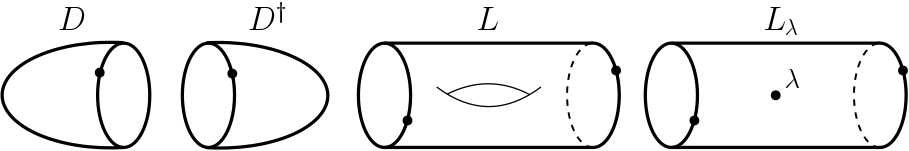 Figure 1
Peer Reviews
No public reviews on file for this paper yet. If you reviewed it on a platform where reviews are public (OpenReview, ICLR, NeurIPS, ICML), you can paste yours below so the community can read it here.
Videos
No videos yet. Explain this paper in a talk, walkthrough, or lecture? Add one.
Virtual classes of
parabolic -character varieties
Ángel González-Prieto
Instituto de Ciencias Matemáticas CSIC-UAM-UC3M-UCM. C. Nicolás Cabrera, 13-15, 28049. Madrid, Spain.
ETSI de Sistemas Informáticos, Universidad Politécnica de Madrid. C. Alan Turing s/n, 28031. Madrid, Spain.
Abstract.
In this paper, we compute the virtual classes in the Grothendieck ring of algebraic varieties of -character varieties over compact orientable surfaces with parabolic points of semi-simple type. When the parabolic punctures are chosen to be semi-simple non-generic, we show that a new interaction phenomenon appears generating a recursive pattern.
1. Introduction
††footnotetext: 2010 Mathematics Subject Classification. Primary: 14C30. Secondary: 57R56, 14L24, 14D21. Key words and phrases: TQFT, character varieties, Geometric Invariant Theory.
Let be topological space with finitely generated fundamental group, , and let be a reductive algebraic group. The set of representations of into , , has naturally a structure of algebraic variety, the so-called -representation variety of and denoted . Moreover, the group itself acts on by conjugation so we can consider the associated Geometric Invariant Theory (GIT) quotient, , called the -character variety of . Since two representations are equivalent if and only if they are conjugated, the character variety is the moduli space of representations of into [24].
The topology and geometry of character varieties is an active research area. One of the the reasons of this interest is the celebrated non-abelian Hodge correspondence. It states that, if is a closed orientable surface and , then the character variety of is diffeomorphic to the moduli space of rank vector bundles on with fixed determinant and equipped with a flat connection [30, 31], and to the moduli space of rank and degree [math] Higgs bundles on with fixed determinant [4, 29]. Despite that the three moduli spaces are naturally complex algebraic varieties, the correspondences are not holomorphic. This endows with three different complex structures that give rise to the first non-trivial example of a hyperkähler manifold [14].
For this reason, a thorough analysis of the natural algebraic structure on is needed. However, even in the simplest cases, the problem is very hard. The first approach was accomplished by Hausel and Rodríguez-Villegas in [13]. There, they introduced an arithmetic method that computes the -polynomial of the -character variety by counting its number of points in finite fields, in the spirit of the Weil conjectures. In [22], Mereb extended the results to the case . This strategy has also been exploited in [26], [27] and [20] at the side of the moduli space of Higgs bundles.
Despite of the power of the arithmetic method, it is a pure combinatorial approach that barely gives information about the underlying geometric structure of the character variety. In this way, Logares, Muñoz and Newstead in [16] initiated a more geometric approach to the computation of -polynomials of character varieties. The key idea of this paper is to chop into simpler pieces for which the -polynomial can be easily computed. Then, using the additivity of the -polynomial, the polynomial of the whole space can be obtained by summing up all the contributions. Finally, they understood the identifications that appear in the GIT quotient to get the -polynomial of .
Using this method, for , in [16] it is explicitly computed the -polynomial of the character variety over a surface of genus and , in [17] for genus and in [18] for arbitrary genus. Moreover, in [1], using a mix between the arithmetic and the geometric method, it was computed the -polynomial of character varieties over orientable surfaces for and over non-orientable surfaces for .
An even harder challenge appears when we consider a parabolic structure on . Roughly speaking, it is given by a set of tuples , where is a collection of different marked points, called the punctures, and is a collection of conjugacy classes of elements of , called the holonomies. In this case a -parabolic representation is a representation such that, if is the loop around the puncture , then . The set of -parabolic representations also form an algebraic variety , called the parabolic -representation variety of . The corresponding GIT quotient is the moduli space of -parabolic representations, known as the parabolic -character variety. The non-abelian Hodge correspondence extends naturally to the parabolic setting to give diffeomorphisms with the moduli space of logarithmic flat connections and with the moduli space of parabolic Higgs bundles [28].
However, very little is known about the algebraic structure of character varieties in the parabolic case. One of the most important advances was done in [19] and [21] for , where the -polynomial is computed for parabolic structures of generic semi-simple type i.e. the holonomy conjugacy classes are orbits of semi-simple elements lying in some Zariski open set of . For general parabolic structures, in [15] the case of at most two punctures in is considered over elliptic curves. However, the arithmetic method is limited to deal with generic punctures. On the other hand, the geometric method is based on very subtle stratifications of the representation varieties that is not clear how to generalize to arbitrary many punctures.
In order to overcome this problem, in [6] a new method was introduced based on Topological Quantum Field Theories (TQFTs) in the context of the PhD Thesis project of the author [7]. This method exploits the recursive nature of character varieties that is widely presented in the literature [3, 5, 12, 23]. The key idea of this method the following. Let be the category of mixed Hodge structures and let be its associated Grothendieck ring (a.k.a. -theory ring). Let us also consider the category of -dimensional bordisms of pairs with parabolic data in a collection of conjugacy classes of (see Section 2 for a precise definition). Then, in [6], we constructed a lax monoidal functor computing the virtual Hodge structure (i.e. the image in ) of parabolic -representation varieties with holonomies in . Recall that this means that, if is a closed connected -dimensional manifold, is a basepoint and is a parabolic structure on then, seen as a bordism , we have that satisfies .
As an application, in [8] we used this method to compute the virtual Hodge structure of parabolic -representation varieties over orientable surfaces of arbitrary genus and any number of punctures with Jordan-type holonomy. For this purpose, we showed that all the computations of the lax monoidal TQFT can be performed within a finitely generate -module, , called the core submodule. This simplifies the calculations since, in that case, the TQFT can be described explicitly by computing the images of finitely many elements. Using the results of [9] about stratification of GIT quotients, we translated these results to give the virtual Hodge structures of -character varieties over surfaces of arbitrary genus an any number of punctures of Jordan type.
Nonetheless, if we consider semi-simple holonomies in the parabolic structure, the situation becomes much more involved. The most important problem is that the semi-simple punctures trigger the appearance of new generators of the submodule , so it is no longer invariant under the TQFT. Moreover, if the punctures are not generic, an interaction phenomenon arises between these new generators. The aim of this paper is to explore this case.
In Section 2, we will sketch briefly the construction of [6] of the lax monoidal TQFT, . Moreover, we will show that, with a small modification, we can improve this TQFT to compute, not only virtual Hodge structures on representation varieties, but indeed the virtual class of the representation variety . Here is the localization of the usual Grothendieck ring of complex algebraic varieties, , by a certain multiplicative set. This extension is compatible with the description of the TQFT in [6] and those computations can be translated directly to this new context.
Section 3 is the core of this paper. There, we perform the computation of the TQFT for and punctures of semi-simple type. For this purpose, we explicitly identify the new generators induced by the semi-simple punctures. In Section 4, we perform the computation of the TQFT for the tube with a single puncture with semi-simple holonomy and we express the result in terms of the new generators. In Section 4.13, we extend the computations of Sections 6.3 and 6.4 of [8] to the new set of generators, completing the explicit description of the TQFT. Finally, in Section 5 we address the interaction phenomenon, giving rise to a combinatorial formula that shows how to modify the generic virtual class to deal with the case of non-generic punctures. These interaction phenomena are at the bottom of the reason why the arithmetic method breaks down when considering non-generic punctures. Therefore, as a consequence of these computations, in Theorem 5.6 we obtain the following result.
Theorem**.**
Let be the closed orientable genus surface and fix traces , maybe non-generic. Write them as for some . Let (resp. ) be one half of the number of tuples such that (resp. such that ). Let be a parabolic structure with punctures with holonomy and punctures with holonomies . Denote and let be the localization of with respect to the multiplicative set generated by and . The virtual class of in is
- •
If , then
[TABLE]
where the interaction term is given by
[TABLE]
- •
If , then
[TABLE]
where the interaction term is given by
[TABLE]
Finally, in Section 6 we use the techniques of [9] to translate this result across the GIT quotient down to character varieties. For this reason, in Section 6.1 we review the theory of pseudo-quotients that allows stratifications of representation varieties. In Section 6.3 we apply this theory to count the identifications that take place in the GIT quotient of the parabolic representation variety. In this way, we finally obtain the following result (Theorem 6.1).
Theorem**.**
The virtual class of in is
- •
If , then
[TABLE]
- •
If , then
[TABLE]
Also, we will show how the remaining combinations of holonomies for the punctures can be reduced to one of these cases of the ones studied in [8, 9].
This result finishes the study of virtual classes of parabolic -character varieties. However, much remain to be done in this business. First, the next goal would be to extend these results to higher rank. The case would allow us to extend the results of [1] to the parabolic case and the case is completely unknown. We expect that these situations might be addressed with the techniques developed in this series of papers. Furthermore, it would be interesting to consider other families of groups as or to explore the similarities and differences in the corresponding TQFTs. This study will be relevant towards the understanding of the mirror symmetry conjectures for character varieties, since and are Langlands dual groups.
The next step would be to extend the TQFT used here to deal with representation varieties over more general spaces. In particular, it would be interesting to consider the case of character varieties over singular and non-orientable surfaces, as well as over complements of knots. This is the objective of a upcoming paper.
A more ambitious goal would be to extend the TQFT across the non-abelian Hodge correspondence to compute also virtual classes of moduli spaces of flat connections and moduli spaces of Higgs bundles. This would allow us to capture not only a particular complex structure but the whole picture of the hyperkähler structure. Finally, we expect that the TQFT constructed will be useful to shed some light into the mirror symmetry conjectures for character varieties posed in [10] that predict some astonishing symmetries of -polynomials of character varieties over a group and its Langlands dual group .
Acknowledgements
The author wants to thank Tamás Hausel, Anton Mellit, Peter Newstead and Thomas Wasserman for very useful conversations. I would also like to express my highest gratitude to my PhD advisors Marina Logares and Vicente Muñoz for their invaluable help, support and encouragement throughout the development of this paper.
The author acknowledges the hospitality of the Faculty of Mathematical Sciences at Universidad Complutense de Madrid, in which part of this work was completed. The author has been supported by a ”la Caixa” Foundation scholarship LCF/BQ/ES15/10360013 and partially by a MINECO (Spain) Project MTM2015-63612-P.
2. Topological Quantum Field Theory for representation varieties
In this section, we shall sketch briefly the construction of the TQFT described in [6]. We will also include some modifications that will allow us to compute, not only virtual Hodge structures, but the whole virtual class in the Grothendieck ring of algebraic varieties.
We will follow the notation of [6]. Let be a set, and let be the category of -bordisms of pairs with parabolic data in . Recall that an object of this category is a triple with a closed -dimensional manifold, a finite set meeting each connected component of and a parabolic structure on , i.e. a set of co-oriented disjoint submanifolds of codimension , with labels .
A morphism is given by a unoriented bordism between and , a finite set of points meeting each connected component of and such that and , and a parabolic structure on such that the restrictions on and agree with and , respectively. Composition of morphisms is given by gluing of bordisms along their common boundary and juxtaposition of basepoints and parabolic structures. The category is naturally a monoidal category with monoidal product the usual disjoint union of manifolds.
Now, let be a commutative and unitary ring, and let be the category of -modules and -module homomorphisms. A lax monoidal Topological Quantum Field Theory, shortened TQFT, is a lax monoidal functor
[TABLE]
Remark 2.1*.*
The lax monoidality condition means that, for any , there exists a -module homomorphism
[TABLE]
However, this morphism might be not an isomorphism, in contrast to what is mandatory for a genuine monoidal functor.
Remark 2.2*.*
We can endow and with natural -category structures. In this framework, a lax monoidal TQFT can be usually promoted to a -functor. However, for computational purposes, we will not need this structure, so we will not explore it further in this paper. For more information, see [8].
A closed -dimensional manifold , together with a finite set and a parabolic structure on it, defines a morphism . Hence, under the TQFT, it gives rise to a -linear map . This map is fully determined by the element that we can think as an algebraic invariant of . In this sense, we say that computes the invariant .
2.1. Standard TQFT
In [6], it was constructed a lax monoidal TQFT that computes virtual Hodge structures of representation varieties. Such TQFT was constructed by means of a ‘pull-push construction’ by splitting the TQFT into a ‘field theory’ and a ‘quantisation’, being the later constructed via a -algebra (for a review of this method and these concepts, see [8, Section 4]). In this section, we will slightly extend this construction to compute the whole virtual class of the representation variety in the Grothendieck ring of algebraic varieties.
Let us fix a ground field . Let be the category of algebraic varieties over with regular morphisms between them. Moreover, given , we will denote by the relative category of algebraic varieties over . Recall that the objects of this category are pairs with and algebraic variety and a morphism . If the morphism is clear from the context, the object will be denoted just by . Given objects , a morphism between them is a regular morphism such that . Finally, we will consider the associated Grothendieck rings (also known as the -ring in -theory), and . The image of an algebraic variety in the Grothendieck ring will be denoted and will be called the virtual class of .
Now, fix an algebraic group and let be a collection of subvarieties of that are invariant under conjugation (e.g. conjugacy classes of some elements). Given , we are going to construct a lax monoidal TQFT, such that, for all morphism , it gives
[TABLE]
This TQFT is called the standard TQFT. In order to construct this functor, we are going to split it into two functors
[TABLE]
Here, is the category of spans of (see [2] for the definition). The functor is playing the role of a field theory and is playing the role of a quantisation (in the physical sense).
The field theory, , coincides with the one described in [6]. On an object , it assigns , the associated parabolic -representation variety of the fundamental groupoid (see Remark 2.3). Also, given a bordism , it assigns the span
[TABLE]
Here, and are the maps induced by the inclusions and , respectively, at the level of representations. By the Seifert-van Kampen Theorem for fundamental groupoids, is a well-defined functor.
Remark 2.3*.*
Recall that, given a compact manifold and a parabolic structure , the set of -parabolic representations, , has naturally the structure of an algebraic variety. Suppose that is the parabolic structure. Roughly speaking, the algebraic structure comes from considering a finite set of generators of , with the loops around the submanifold in the positive direction given by the orientation of the normal bundle of . Then, we identify with the image of the map , , that is an algebraic set.
In the case of having a set of basepoints , we can consider the representation variety of representations of the fundamental groupoid such that if is a positive loop around . In that case, by picking a distinguished element on each component of , we have a natural identification , where are the connected components of meeting a basepoint. This also endows with the structure of an algebraic variety. This is the structure considered along this paper.
The quantisation part is slightly different from the one in [6]. We will construct it by means of a -algebra (see [8, Section 4.1]) given by the following data.
- •
On an object , it assigns , the Grothendieck ring of algebraic varieties relative to . It is a ring with product the fibered product of varieties.
- •
In particular, the image of the singleton variety (i.e. of the final object) is . In this way, also has a natural -module structure by cartesian product.
- •
Given a regular morphism , we define to be morphism given by for . Analogously, we define by , where is the map fitting in the pullback diagram
[TABLE]
Observe that is a -module homomorphism by its very definition, as it commutes with cartesian product. Moreover, is a ring homomorphism since , for any , and analogously for the corresponding regular morphisms.
By the usual base change property for algebraic varieties, this assignment has the Beck-Chevally property. Thus, it is a -algebra that we shall denote . Therefore, by [8, Theorem 4.13], it gives rise to a lax monoidal functor . By construction, to a span of the form , it assigns the homomorphism such that . Thus, putting together this quantisation functor with the field theory, we have obtained the following result.
Theorem 2.4**.**
Let be an algebraic group and . There exists a lax monoidal TQFT
[TABLE]
computing virtual classes of parabolic -representation varieties.
2.2. Recovering Hodge monodromy representations
Suppose that the ground field is . In that case, we can also consider the -algebra of the -theory of mixed Hodge modules, , as in [6, 8]. In order to avoid misinterpretation with the maps of , the induced maps of will be denoted and . Note that this slightly differs from the notation of [6, 8].
Using as the -algebra for the quantisation, we also obtain a lax monoidal TQFT that we will denote . Here is the category of rational mixed Hodge modules. This was the TQFT used in [8] for calculations.
This functor and the functor constructed here are strongly related. To state the relation properly, suppose that we are working in a category with pullbacks and final object. Let and be two -algebras. In particular, this means that are contravariant functors out of with values in rings, and are covariant functors out of with values in modules over the rings , respectively. By a natural transformation , we will refer to a collection of ring homomorphisms , for , intertwining with the induced maps. This means that, for any morphism of , we have and .
Proposition 2.5**.**
Let . Consider the morphism that, for , sends , where denotes de unit of the ring. Then defines a natural transformation of -algebras
[TABLE]
Proof.
The maps intertwine with the induced maps of the -algebras. In order to check it, let be a regular morphism. For the pushout, we directly have . For the pullback map, consider the cartesian square
[TABLE]
By the Beck-Chevalley property of , we have
[TABLE]
Observe that, in the third equality, we have used , since is a ring homomorphism.
Finally, let us show that the maps are ring homomorphisms. Suppose that and are objects of . If denotes the diagonal map, and denotes the usual cartesian product (i.e. the fibered product over ), we have a cartesian square
[TABLE]
By definition, we have .
On the other hand, let us denote the projections onto the first and the second component, respectively. Since , we have that
[TABLE]
Note that, in the last equality, we have used . Therefore, by the Beck-Chevalley property of , both elements agree. This proves that is a ring homomorphism. ∎
Remark 2.6*.*
- •
The mixed Hodge module first appeared in [16] (see also [18]), where it was called the Hodge monodromy representation and was denoted by , or if the map was clear from the context. In this notation, the intertwining property reads and . Moreover, the fact that is a ring homomorphism implies that .
- •
The fact that is a ring homomorphism is quite surprising since, for a regular map , the morphism is not in general a ring homomorphism. However, it preserve the external product, that was exactly what we needed in order to complete the proof above.
In particular, the natural transformation gives us a ring homomorphism . It induces a natural transformation . Under this transformation, can be seen as taking values in . With these considerations, we have the following result.
Corollary 2.7**.**
There exists a natural transformation given by , for .
Proof.
By the construction of both functors, it is enough to build the natural transformation at the level of the respective quantisations, denoted . For this purpose, we can just take , for an algebraic variety . Unraveling the definitions, we get the claimed formula. ∎
2.3. Geometric and reduced TQFTs
Despite that computes the virtual class of representations varieties, it is convenient to consider a modification of this TQFT that is easier to compute. It is produced by the reduction procedure described in [8, Section 4.5]. In this Section, we will sketch the construction of this modification and we will describe the associated maps explicitly.
Given , there exists an action of on by conjugation. The orbit space of this action can be given the structure of a piecewise algebraic variety (see [8, Section 5.2]), denoted . We also have a piecewise algebraic quotient map .
With this piecewise quotient, we modify the field theory to assign, to any morphism of , the span
[TABLE]
Using this new field theory and the quantisation induced by the -algebra , we obtain a new assignment called the geometric TQFT.
Unfortunately, in this form is not a genuine functor since the new field theory does not satisfy the Seifert-van Kampen theorem. Nevertheless, this problem can be easily solved. Consider the endomorphism
[TABLE]
If is invertible then, by [8, Proposition 4.20], is a lax monoidal TQFT computing the same invariant than , called the reduced TQFT. For this reason, we can focus on the computation of the geometric TQFT, from which the reduced TQFT follows immediately.
Remark 2.8*.*
It may happen, and it will be actually the case in our computations of Section 3, that is not invertible directly. However, suppose that there exists a multiplicative set such that is actually invertible. In that situation, we can still get a reduced TQFT that, now, it will compute the virtual class of the representation variety in the localized ring .
In the case , we can give explicitly the morphisms associated to the geometric TQFT. Observe that, in this case, the boundaries have no parabolic structures since the parabolic structure are codimension submanifolds. Now, consider the set of morphisms of depicted in Figure 1, for .
The importance of these bordisms is the following. Let be the orientable closed surface of genus and consider any parabolic structure on it with marked points. Then, if is a set of basepoints of , as a morphism we can decompose . Thus, in order to compute virtual images of representation varieties over closed surfaces, we can only focus on this special set of bordisms.
With respects to the boundaries, we only need to care about the circle with a single basepoint, . We have that the associated module is i.e. Grothendieck ring of varieties over the set of conjugacy classes of . In order to get in touch with the notation of Section 3, let us denote this piecewise quotient map as . With respect to morphisms, as explained in [8, Section 5.1], the associated field theories of the discs are
[TABLE]
[TABLE]
Therefore, and . On the other hand, for the tubes and , the associated field theories are
[TABLE]
[TABLE]
Hence, and . Finally, the reduced TQFT is with .
3. Parabolic -representation varieties
From now on, we shall focus on the case of surfaces and , for which we will compute the module homomorphisms of the reduced TQFT, as described in the previous section. This is analogous to the results of [8] but for a wider set of allowed holonomies for the punctures. For convenience, we will shorten by .
3.1. Generalities on
In order to fix notation, recall that in there are five special types of elements, namely the matrices
[TABLE]
with . Any element of is conjugated to one of these elements. Such a distinguished representant is unique up to the fact that and are conjugated for all . Hence, we have a stratification
[TABLE]
where and denotes the conjugacy class of . Given , we will also denote .
The GIT quotient of the action of on itself is given by the trace map . By the stratification above, it only identifies the orbits and (both orbits of matrices of trace ) as well as the orbits and (both orbits of matrices of trace ). This implies that the piecewise quotient space is
[TABLE]
where is the space of traces of matrices with two different simple eigenvalues. The orbitwise quotient map will be denoted . Under the action of on itself by conjugation we have that , and , for . In particular, if we denote , we have that , and (see [8, Section 6] for details).
In analogy with [8, Section 6.1], under the inclusion of these strata into , we can consider the respective units , , , and seen as elements of . On , we also consider the varieties
[TABLE]
Let be their projections onto the second component, . In this setting, the pairs and define elements of that we will denote and , respectively. We set and . It can be proven that, if we consider , with projection over given by , then , where denotes the product in . These elements satisfy some algebraic relations in that we will need for the subsequent computations.
Lemma 3.1**.**
In the ring , the following relations hold.
[TABLE]
Proof.
For the first equality, observe that it holds
[TABLE]
Therefore, we have that and, solving for , we find . The computation for is analogous. The second equality can be obtained directly from this result, since we have
[TABLE]
However, a more directed proof can be given. Using the explicit expression of , we have that
[TABLE]
Observe that, in the second equality, the isomorphism is given by the map . ∎
The importance of these elements comes from the fact that, in [8], it was proven that the submodule generated by is invariant under and and that and are respectively the inclusion and projection onto . This means that all the computations of the TQFT can be safely restricted to this submodule.
For the purposes of this paper, we also need to consider a kind of ‘skyscraper generators’ over selected points of . For , we shall denote by the image of the unit in . In this way, we will consider the -submodule generated by and all the skyscraper generators for , that we will denote . Observe that is not finitely generated, in contrast to .
Remark 3.2*.*
There is a small change of notation with respect to [8, Section 6.1]. In that paper, the elements and are denoted as and , respectively. We have decided to change notation in order to avoid the ambiguity of using to denote both the unit over and over the matrices of trace . With the new convention, always refers to the unit over , the diagonalizable matrices of trace .
Another minor change of notation is that in this paper stands for what it was denoted as in [8]. This change allows us to be consistent with the product notation in the quantisation ring, that is cartesian product of varieties in this paper but it was tensor product of mixed Hodge modules in [8].
Let us consider the module endomorphism . The image under this map of was calculated in [8]. Taking into account the new skyscraper generators, we have the following result.
Lemma 3.3**.**
The submodule is invariant for the morphism . Indeed, the image of is given by and, with respect to the standard set of generators, the matrix of is
[TABLE]
Proof.
We just need to compute the image of the new skyscraper generators. Fix . We have a commutative diagram whose square is cartesian
[TABLE]
Hence, we have that . Combining this computation with [8, Proposition 6.3], the result follows. ∎
Remark 3.4*.*
The morphism is not invertible, as the polynomials in appearing the the matrix above are not units of . However, is invertible as endomorphism of the localization of with respect to the multiplicative set generated by and . From now on, we will denote the localizations for a complex algebraic variety and, in particular, we set . In this way, we get that is invertible. As mentioned in Remark 2.8, this implies we can still carry on our computations on the corresponding localized Grothendieck rings.
3.2. The semi-simple puncture
Fix and write for some . In this section, we shall compute the image of the tube under the reduced TQFT, where . Recall that the field theory for on is the span
[TABLE]
so .
Instead of the orbit space required by the field theory, it will be also convenient to consider the rough GIT quotient span
[TABLE]
Taking into account that , we get that this span is naturally isomorphic to
[TABLE]
Since the second and the third factors play no role in the previous span, we can focus on the simplified span
[TABLE]
Lemma 3.5**.**
Let be the algebraic variety
[TABLE]
Then, span (1) is isomorphic to
[TABLE]
Moreover, let us decompose where and . Then we have
- •
* is isomorphic to and the maps of the span correspond to the projections onto the second and third components, respectively.*
- •
* is isomorphic to . Under this isomorphism, the span is*
[TABLE]
Proof.
Let us take
[TABLE]
A straightforward computation shows that is the set of matrices of the form
[TABLE]
satisfying that
[TABLE]
With this description, we have that the left-most span map corresponds to , and the right-most map to . On , we can solve this equation for and the span maps are trivial fibrations with fibers .
If , the later equation forces and to satisfy
[TABLE]
Hence, is an affine hyperbola that can be parametrized by , . Under this isomorphism, the maps and become the claimed maps and , respectively. ∎
Proposition 3.6**.**
On , the endomorphism is given by
[TABLE]
Proof.
Observe that and . Hence, the span for restricts to
[TABLE]
Consider the isomorphism given by , the map and the projection . We can write and so we have that , with .
In particular this implies that, for , it holds since and are ring homomorphisms. For , we have that , which is isomorphic to as element of . Therefore, we have that and analogously for and . Thus, does not modify the calculation and we can focus on the computation of .
In this case, observe that we have an isomorphism , given by . Under this isomorphism, there is a commutative diagram
[TABLE]
where is . Since is an isomorphism, . In particular, we have that . On the other hand, Lemma 3.1 implies that
[TABLE]
and analogously for . For , also using the relations of Lemma 3.1 we obtain
[TABLE]
Therefore, using that , and subtracting the missing fibers over , the result follows. ∎
4. Computations of the geometric TQFT
After the preliminary computations of Section 3, we are ready to accomplish the computation of the geometric TQFT. Along this section, we fix and we write it as for a fixed . We shall focus on the computation of the -module morphism
[TABLE]
For short, if are subvarieties of , we shall denote
[TABLE]
We will also write so , where .
4.1. Image of
We have that and is just the projection onto a point . Hence, .
4.2. Image of
Analogously to the previous case, we have that and is the projection onto the point so .
Remark 4.1*.*
In general is not conjugated to except in the case . In that case, so .
4.3. Image of
In this case, has a non-trivial decomposition. Analyzing the strata separately we obtain the following.
- •
Over , we have that so these strata add no contribution.
- •
Over , a direct computation shows that
[TABLE]
This agrees with the calculation of Lemma 3.5. Therefore, .
- •
Over , by Lemma 3.5 we have that
[TABLE]
and is given by . Where , the previous equation forces . We have to remove the point from the fiber , so this stratum contributes as . Where , we can solve for and is free, so this stratum contributes as . Hence, we have that .
Adding all the contributions of the strata, we finally have that
[TABLE]
4.4. Image of
The calculations for this stratum are completely analogous to the ones for so we find that
[TABLE]
4.5. Image of
As in the previous case, we stratify and analyze each piece separately.
- •
Over , we have and is the projection onto a point. So we obtain that .
- •
Over , by Lemma 3.5, we have that
[TABLE]
Observe that we have to remove the point , for which instead of . This corresponds to . Where , we know by Lemma 3.5 that the fiber is that contributes with . Where , we have so the fiber is that contributes with . Taking into account the factor we obtain that .
- •
Over , analogously we have that
[TABLE]
As proved in Lemma 3.5, with respect to the projection onto , we have that for it is a trivial fibration of fiber so this part contributes with . On the other hand, the stratum contributes with .
Adding up the contributions, we find that
[TABLE]
4.6. Image of
The computation for this generator is very similar the previous one but taking into account the double cover that defines . We shall focus on the computation of and, using that the result follows by calculating .
According to the stratification of we have
- •
Over we have the commutative diagram with cartesian square
[TABLE]
where . Using that we find that so . This implies that
- •
Over , we a commutative diagram
[TABLE]
where . Stratifying according to as in Lemma 3.5 we have the following strata.
- –
For , the equation for in Lemma 3.5 forces that . In this way, we have that
[TABLE]
Therefore, .
- –
For , we can solve for to obtain that
[TABLE]
The first factor is an affine parabola without points so we have that .
Adding up all the contributions, we find that and, thus, .
- •
Over , the computation is completely analogous and we have .
- •
Over , the commutative diagram
[TABLE]
is completed with
[TABLE]
The projection becomes . As above, we stratify depending on .
- –
Where , the situation is simple since we can solve for and thus
[TABLE]
Moreover, under this isomorphism the map becomes the projection onto the last component. Therefore, since , we obtain that .
- –
Where , by Lemma 3.5 we get that this stratum contributes as .
Adding up all the contributions and subtracting , we finally find that
[TABLE]
4.7. Image of
The calculations for this element are analogous for the ones of , so we also obtain
[TABLE]
4.8. Image of
The computation for this element is very similar the one of . As above, we will compute and, using that , we get the image of as .
As above, we decompose the calculation according to the stratification of .
- •
Over we have the commutative diagram with cartesian square
[TABLE]
where the pullback variety is given by
[TABLE]
Therefore, we get .
- •
Over , there is a commutative diagram
[TABLE]
where . Stratifying according to , we get
- –
For , the equation for in Lemma 3.5 forces that and, thus
[TABLE]
Therefore, .
- –
For , we solve for so that
[TABLE]
The first factor is an affine hyperbola minus points, that contributes with . Therefore, .
Adding up all the contributions, we find that and, thus, .
- •
Over , the situation is completely analogous to the previous item so we have that .
- •
Over , we have the commutative diagram
[TABLE]
that is completed with . As always, we stratify depending on .
- –
Where , we get a trivial fibration as for with fiber so we obtain that .
- –
Where , by Lemma 3.5 we get that this stratum contributes as .
Therefore, putting together these results we find that
[TABLE]
4.9. Image of
- •
Over , we have that , so we have that .
- •
Over , we have that , except in the case that for which (c.f. Remark 4.1). Hence, if and .
- •
Over , the calculation is a simplified version of the one in Section 4.5. On , having and implies that . Hence, so .
- •
Over , now we have that, in , to have and implies that for some fixed. If , then . Thus so . However, if then and we have the same situation as for , so .
- •
Over , we also have a simplified version of Section 4.5. In this case, is given by the tuples such that
[TABLE]
- –
For , this equation forces . Hence, this stratum contributes as if , and [math] if .
- –
For , we can solve the equation for and we get , being the map the projection onto the first component. Thus, this stratum contributes with .
Adding up all the contributions, we get that, for
[TABLE]
On the other hand, in the case we obtain
[TABLE]
4.10. Image of
The computation for this generator is analogous to the one of . The differences are that, now, the stratum for is empty, except in the case , and the fibration over in the case lands in . Taking into account these changes, we obtain that, for
[TABLE]
Remark 4.2*.*
In the case , the generators and are indistinguishable, so both calculations of Sections 4.9 and 4.10 must apply. For this reason, has to be symmetric in and . This explains the balanced shape of .
4.11. Image of with
- •
Over , we have that , so these strata add no contribution.
- •
Over , we have that . In particular, since , the product so we can solve for . Hence, we obtain that so these strata contributes with .
- •
Over , we have that .
- –
For , is forced to be one of the two (different) roots of the equation for in Lemma 3.5, namely . Hence, this stratum contributes as .
- –
For , we can solve this equation for and we get , being the map the projection onto the first component. Thus, this stratum contributes with .
Therefore, taking into account all the contributions, we finally get that
[TABLE]
Remark 4.3*.*
The new traces can be better understood as follows. Let us consider the eigenvalues of and write it as , for . Then, the two new traces are the ones associated to the eigenvalues and , that is, and (or vice-versa, the names are arbitrary). In particular, for we have that and . Since we have to dismiss the root , we only have one contribution in Sections 4.9 and 4.10.
4.12. The reduced TQFT
From the computations of the previous sections, we have obtained an explicit expression of the morphism on . With this information at hand, passing to the localization with respect to and as mentioned in Remark 3.4, we can finally compute the reduced TQFT, .
Theorem 4.4**.**
Fix . Under the module homomorphism , we have that . Explicitly, in the set of generators, the matrix is
[TABLE]
In the case , the images of or with are the same as above, but the image of is given by
[TABLE]
Proof.
From the computations above, we know the explicit expression of . The reduced TQFT is . Thus, as , the same holds for . Moreover, from the expression of given by [8, Proposition 6.3] and Lemma 3.3, the matrix of can be explicitly computed using a computer algebra system. ∎
4.13. Image of under other tubes
Once completed the computation of , we need to extend the calculations in Sections 6.3 and 6.4 of [8] for and to the whole . Since the image of the generators of is known [8, Theorem 6.5], it is enough to compute the elements , and .
This task can be performed following the strategy of the previous sections, but there is a shortest path that we shall explain here. By Theorem 4.4, we have . Now, observe that the bordisms and commute as morphisms of so . Therefore, since and , we get that
[TABLE]
These last term can be computed from the expression of in [8, Theorem 6.5] and Theorem 4.4 for . Moreover, analogous arguments hold for the bordism . Putting together this information we obtain the following result.
Proposition 4.5**.**
The image of under the endomorphisms and is
[TABLE]
Remark 4.6*.*
As in the case of Theorem 4.4, from this information and the explicit expression of the endomorphism , we can easily compute the reduced versions and .
5. The interaction phenomenon
The previous computation shows that there exists a dichotomy in the behavior of the TQFT on the skyscraper generators over . Fix and consider the tube . As shown in Theorem 4.4, for , the images of the generators under are
[TABLE]
Therefore, these images are essentially equal with varying . However, for the image has a different shape
[TABLE]
We can interpret this last element as follows. In this case, we have that but . Hence, one of the two new skyscraper generators lies over the matrices of trace i.e. . In this way, the contribution that appears in the generic case becomes in the case . We may understand this phenomenon as that the trace interacts with the generator destroying the element and creating two new elements and . Analogous considerations can be done for , where is destroyed and a new contribution appears.
This ‘interaction phenomenon’ makes the computation of the iterated element much more involved that the non-semisimple case of [8]. In this section, we shall study thoroughly this interaction phenomenon and we shall provide an explicit formula for the iterated element.
5.1. The generic part
Let us consider in the first place the generic case. The importance of this situation is that, for generic traces , we can obtain a closed formula for the image of the bordism .
Definition 5.1**.**
Let be traces, and let us write them as for some . We will say that they are generic if all the products for all .
Remark 5.2*.*
This definition of genericity agrees with the Definition 4.6.1 of [21]. However, as we will see, we came up to this definition guided through a different path.
With a view towards the following result, for simplicity let us denote by the map . This is the quotient map for the action of on by , i.e. permutation of the eigenvalues.
Proposition 5.3**.**
Let be a generic set of traces, and let us write them as for some . Then we have
[TABLE]
The coefficients are given by
[TABLE]
Proof.
The formulae for the coefficients and follow easily by an induction argument using the matrix of Theorem 4.4. For the coefficients of the skyscraper generators for , the key point is to observe that the linear relation holds for any . Hence, working by induction we have that
[TABLE]
The formula for the skyscraper generators follows from the observation that, for any , we have . ∎
5.2. The interaction term
Despite our success in the computation of the generic situation, we still need to correct this result to take into account the contribution in the non-generic case. For this purpose, suppose that we have traces and let us write them as for . We shall denote
[TABLE]
If we need to make explicit the set of traces over which is computed, we will write .
In this situation, we define the interaction term of the traces as
[TABLE]
Observe that does not depend on the chosen ordering of the traces nor the choice the eigenvalue or for . Hence, indeed it only depends on the set of traces.
The importance of this term comes from the following result.
Proposition 5.4**.**
Let be any traces. Then we have
[TABLE]
where the sum on the skyscraper generators runs over the set of tuples such that .
Proof.
Firstly, observe that, if are generic, then and the result follows from Proposition 5.3. We will prove the result by induction on . For the base case , the formula holds since this case is always generic.
In the general case, we may suppose that is not generic with . For simplicity, let us denote and . Observe that, if we shorten and , then the number of times that appears in is precisely . Now we separate the sum as
[TABLE]
When we compare with respect to the image of the same sum in the generic case, we see that each generator gives an extra contribution to the submodule of . This implies a total extra contribution of with respect to the generic case. This justifies the appearance of the new interaction term.
On the other hand, has summands, which is fewer terms than the generic case. This implies that has a missing contribution of to the submodule with respect to the generic case. Moreover, it also creates a deficit of to the submodule generated by the skyscraper generators, coming from the missing terms in satisfying . This missing contribution is offset with the image of the old interaction term, as
[TABLE]
Putting together these observations, we finally get that
[TABLE]
as we wanted to prove. ∎
Remark 5.5*.*
In Definition 5.1, we defined a set of traces to be generic as the property of having no interaction within any subset for . However, Proposition 5.4 proves that, indeed, the final result does not depend on the potential interactions on proper subsets but only on the whole set . This is a quite surprising memoryless property that cannot be expected from the only shape of the TQFT.
Once we know how to control the interaction phenomenon, we can finally give a closed formula for the virtual class of any parabolic representation variety.
Theorem 5.6**.**
Let be the closed orientable genus surface and fix traces , maybe non-generic. Let be a parabolic structure with punctures with holonomy and punctures with holonomies . The virtual class of in is
- •
If , then
[TABLE]
The interaction term is given by
[TABLE]
- •
If , then
[TABLE]
The interaction term is given by
[TABLE]
Proof.
The proof is a computation using the results of [8, Theorem 6.5 and Corollary 6.9] and Proposition 5.4. Let us focus on the case , being the case analogous. In that case, if is a set of base points, we can decompose . Therefore, since , via the reduced TQFT we obtain that
[TABLE]
The computation of was accomplished in Proposition 5.4. Observe that this element lies in the submodule generated by and the skyscraper generators for . This submodule is finitely generated and invariant under the maps and .
Hence, using the computations of and of [8], we can write their matricial expression in the natural set of generators of . Now, we decompose them as and , with and their Jordan forms (that, indeed, are diagonal matrices). Let be the dual form of with respect to the standard generators of . Then, we have that
[TABLE]
Since and are diagonal matrices, the powers and can be computed explicitly. Hence, with the aid of a computer algebra system, the first summand gives the first term in the statement and the second summand gives the interaction term . ∎
Remark 5.7*.*
The formula above for is not valid for the case , since has a non-trivial kernel and, thus, .
Remark 5.8*.*
The previous result applies for a more general class of parabolic structures. Let be the closed orientable surface of genus . Let us denote by the parabolic structure with points with holonomy , points with holonomy , points with holonomy and points with respective holonomies . If is even, then is isomorphic to , which is one of the representation varieties considered in Theorem 5.6. On the other hand, if is odd and , then is isomorphic to , which is also one of the cases considered above. The remaining case of having odd and can also be accomplished, as shown in [8, Theorem 6.11], but in general it gives a different virtual class.
6. Parabolic -character varieties
Let be a complex reductive algebraic group, let be a topological space with finitely generated fundamental group and let be a parabolic structure, with associated representation variety .
The variety parametrizes the set of all the parabolic representations , but it does not take into account that some representations might be isomorphic. Hence, if we want to consider the moduli space of parabolic representations up to isomorphism, we need to quotient by the action of by conjugation. This can be done via the GIT quotient
[TABLE]
This is the so-called -character variety of with parabolic structure . In this section, we will focus on the computation of the virtual class .
6.1. Review of the theory of pseudo-quotients
In [9], it is given an algorithm for the computation of the virtual classes of character varieties in terms of the virtual classes of the associated representation varieties. For the sake of completeness, here we will sketch briefly the method.
The key concept introduced for this aim is the pseudo-quotient. Given a complex algebraic variety with the action of an algebraic group , a pseudo-quotient of by is a complex algebraic variety with a surjective -invariant regular morphism such that, for any disjoint -invariant closed sets , the Zariski closures of and in are disjoint. It may be understood as a week version of a good quotient (in the GIT sense [25]) in which we get rid of the condition that is a categorical quotient of . Pseudo-quotients of an action may not be unique, as shown in [9, Example 3.6]. However, in [9, Corollary 3.10] it is proven that, if are two pseudo-quotients for the action of on , then the associated virtual classes , as elements of . In particular, if admits a GIT quotient , then for any pseudo-quotient of .
However, the key property of pseudo-quotients for our purposes is that they behave well with respect to stratifications. Suppose that is an orbitwise-closed open set. This means that is a Zariski open set such that, for any , the Zariski closure of the orbit of under the action of is also in . In that case, we can decompose with a closed -invariant set. Then, [9, Theorem 4.1] shows that, if and are pseudo-quotients for the action of on and respectively, then . Hence, the virtual class of a pseudo-quotient of can be computed by focusing on the corresponding ones for and .
Finally, another very useful property of pseudo-quotients holds. Suppose that there exists a subvariety and an algebraic subgroup that ‘concentrates’ the information of the quotient of by . More precisely, this means that acts on making it an orbitwise-closed set, that the closure of any -orbit of intersects with and that, for any closed -invariant sets , they are disjoint if and only if the closure of their -orbits on are disjoint. This situation is called a core for the action. Then, in [9, Proposition 4.4], it is proven that if is a pseudo-quotient of by and is a pseudo-quotient of by , then . Hence, we can also focus on the action on the core and, up to virtual class, it has all the information of the global quotient.
6.2. Stratification analysis of character varieties
With the theory of pseudo-quotients at hand, we can easily stratify the action of on the representation variety. Let us denote by and the subvarieties of of reducible and irreducible representations, respectively. We have a decomposition with the first stratum being a closed set and the second stratum being an open orbitwise-closed set ([9, Proposition 6.2]). Hence, we have that
[TABLE]
Now, suppose that is a linear algebraic group (so in particular it is affine). Then, by [9, Proposition 6.4] we have that is a free geometric quotient, where is the group of inner automorphisms of . Applying now [9, Theorem 5.4] we finally get .
Furthermore, suppose that . If is the subvariety of completely reduced representations with respect to the standard basis of (i.e. diagonal matrices), then an adaptation of Proposition 7.3 and Corollary 7.4 of [9] implies that is a core for the action of on . Here denotes the symmetric group that acts on by permutation of eigenvalues. Thus, .
Hence, if we localize by , these decompositions give the formula
[TABLE]
6.3. Semi-simple punctures
From now on, we will consider the case . In order to lighten the notation, we shall omit the group from the notation again. Let be the compact orientable surface of genus . Choose and let be the parabolic structure with punctures with holonomies .
In order to understand the action of on the representation variety , we consider the set of upper triangular representations. Let us take be a tuple of upper triangular matrices with , say
[TABLE]
with , and . Then, we have that
[TABLE]
Therefore, if and only if the following system of equations holds
[TABLE]
As in Section 5.2, in order to control the first condition, we consider the set
[TABLE]
so that .
- •
For the quotient of by , we have that is a core for the action. Since and acts on by , we obtain
[TABLE]
- •
For the calculation of , we stratify taking care of equations (3).
- –
Let be the set of completely reducible representations. Any element of is conjugate to one of the form
[TABLE]
with and . This representation is unique up to permutation of the eigenvalues, so we have a double covering
[TABLE]
Therefore, as shown in [9, Remark 5.3], we obtain
[TABLE]
- –
Let be the set of reducible but not completely reducible representations. In this case, any element is conjugated to one of the form
[TABLE]
with , and where is the hyperplane of given by
[TABLE]
In order to compute its virtual class, we have a fibration
[TABLE]
Here, with the line spanned by . Therefore, we have
[TABLE]
Hence, putting all the computations together we get
[TABLE]
Now observe that, since , it is invertible in . Hence, plugging all these data into formula (2) and using Theorem 5.6, we finally get that
[TABLE]
6.4. Holonomies of general type
Now, apart from the chosen semi-simple holonomies over punctures , let us pick new different points . In this case, we consider the parabolic structure with holonomy over , for , and over all the points .
Observe that, in this case, the action of on the associated representation variety is free since . Thus, all the orbits are isomorphic and this implies that the action is also closed. Therefore, we have that
[TABLE]
With these results at hand, we are ready to finish the proof of the the main theorem of this paper.
Theorem 6.1**.**
Let us fix integers , and traces . Consider a parabolic structure with punctures with holonomy , punctures with holonomy , punctures with holonomies and punctures with holonomies . Set and . The virtual class of in is
- •
If , then
[TABLE]
- •
If , then
[TABLE]
Proof.
If there are no punctures with holonomies or , the result follows from the computations above. In the general case, as we showed in Remark 5.8, if is even (i.e. ) we can cancel the negative holonomies and pairwise and the resulting variety is isomorphic to only having punctures of type .
If is odd (i.e. ), we need to change the traces of the semi-simple holonomies to . The only effect in this case is that so the roles of and are interchanged. ∎
If we interpret as the image in -theory of the mixed Hodge structure on the compactly supported cohomology of (i.e. the Tate structure of weight ), the computations of this paper also give rise to the virtual Hodge structure on character varieties. Under this point of view, the results of this paper agree with the calculations of [8, 9] in the case of punctures of Jordan type.
Moreover, if we interpret as a variable in the polynomial ring , we also obtain the -polynomials of the corresponding character varieties. Under this perspective, the results of this paper agree with the existing computations in the literature. Theorem 6.1 agrees with [15] for at most marked points of semi-simple holonomy and genus (notice that there is a typo in [15] in the case ). The result also agrees with [16, 17, 18] for a single marked point and arbitrary genus of semi-simple type. If the surface has a single marked point of type (the so-called twisted variety) and arbitrary many semi-simple punctures of generic type, this result agrees with [11].
Remark 6.2*.*
The virtual classes of the character varieties with are also known from [18, 9]. To be precise, in these papers the computation is done for the virtual image of the mixed Hodge structure. However, following the lines of this paper, the arguments can be adapted to give the same virtual classes in by interpreting .
The reference list from the paper itself. Each links out to its DOI / PubMed record.
- 1[1] David Baraglia and Pedram Hekmati. Arithmetic of singular character varieties and their E 𝐸 E -polynomials. Proc. Lond. Math. Soc. (3) , 114(2):293–332, 2017.
- 2[2] Jean Bénabou. Introduction to bicategories. In Reports of the Midwest Category Seminar , pages 1–77. Springer, Berlin, 1967.
- 3[3] Erik Carlsson and Fernando Rodriguez Villegas. Vertex operators and character varieties. Adv. Math. , 330:38–60, 2018.
- 4[4] Kevin Corlette. Flat G 𝐺 G -bundles with canonical metrics. J. Differential Geom. , 28(3):361–382, 1988.
- 5[5] Duiliu-Emanuel Diaconescu. Local curves, wild character varieties, and degenerations. Preprint ar Xiv:1705.05707 , 2017.
- 6[6] Ángel González-Prieto, Marina Logares, and Vicente Muñoz. A lax monoidal Topological Quantum Field Theory for representation varieties. Preprint ar Xiv:1709.05724 , 2017.
- 7[7] Ángel González-Prieto. Topological quantum field theories for character varieties. Ph D Thesis. Universidad Complutense de Madrid , 2018.
- 8[8] Ángel González-Prieto. Motivic theory of representation varieties via Topological Quantum Field Theories. Preprint ar Xiv:1810.09714 v 2 , 2018.