Model-Free Practical Cooperative Control for Diffusively Coupled Systems
Miel Sharf, Anne Koch, Daniel Zelazo, Frank Allg\"ower

TL;DR
This paper presents a data-driven, model-free control framework for diffusively coupled systems that guarantees convergence to a formation, using passivity theory and network optimization to find suitable gains.
Contribution
It introduces a novel, data-based method to determine control gains for formation control in passive systems, including strategies to reduce conservatism through iterative sampling.
Findings
Guaranteed convergence to desired formation within an epsilon neighborhood.
A data-driven method to compute control gains based on passivity and network optimization.
Reduction of conservatism via iterative experiments and passivity shortage estimation.
Abstract
In this paper, we develop a data-based controller design framework for diffusively coupled systems with guaranteed convergence to an -neighborhood of the desired formation. The controller is comprised of a fixed controller with an adjustable gain on each edge. Via passivity theory and network optimization we not only prove that there exists a gain attaining the desired formation control goal, but we present a data-based method to find an upper bound on this gain. Furthermore, by allowing for additional experiments, the conservatism of the upper bound can be reduced via iterative sampling schemes. The introduced scheme is based on the assumption of passive systems, which we relax by discussing different methods for estimating the systems' passivity shortage, as well as applying transformations passivizing them. Finally, we illustrate the developed model-free cooperative control…
Click any figure to enlarge with its caption.
 Figure 1
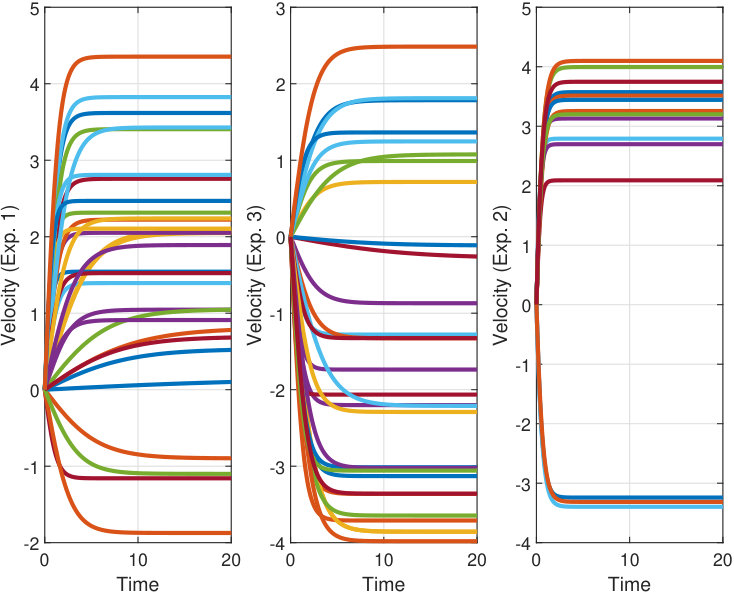 Figure 1
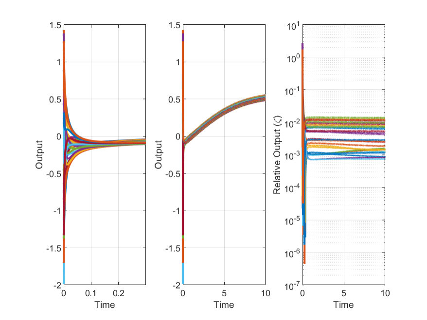 Figure 2
 Figure 4
 Figure 5
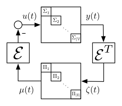 Figure 6
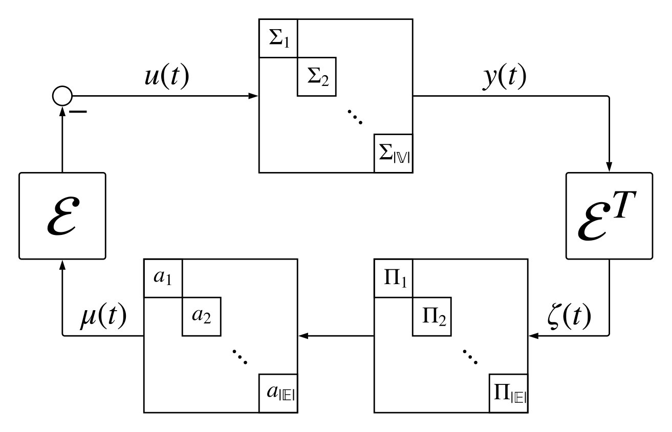 Figure 7
 Figure 8
Peer Reviews
No public reviews on file for this paper yet. If you reviewed it on a platform where reviews are public (OpenReview, ICLR, NeurIPS, ICML), you can paste yours below so the community can read it here.
Videos
No videos yet. Explain this paper in a talk, walkthrough, or lecture? Add one.
Model-Free Practical Cooperative Control for Diffusively Coupled Systems
Miel Sharf, Anne Koch, Daniel Zelazo and Frank Allgöwer M. Sharf is with the Division of Decision and Control Systems, KTH Royal Institute of Technology, Stockholm, Sweden. [email protected]. A. Koch and F. Allgöwer are with the Institute for Systems Theory and Automatic Control, University of Stuttgart, Germany. {anne.koch,frank.allgower}@ist.uni-stuttgart.de. D. Zelazo is with the Faculty of Aerospace Engineering, Israel Institute of Technology, Haifa, Israel [email protected]. This work was supported by the German-Israeli Foundation for Scientific Research and Development.
Abstract
In this paper, we develop a data-based controller design framework for diffusively coupled systems with guaranteed convergence to an -neighborhood of the desired formation. The controller is comprised of a fixed controller with an adjustable gain on each edge. Via passivity theory and network optimization we not only prove that there exists a gain attaining the desired formation control goal, but we present a data-based method to find an upper bound on this gain. Furthermore, by allowing for additional experiments, the conservatism of the upper bound can be reduced via iterative sampling schemes. The introduced scheme is based on the assumption of passive systems, which we relax by discussing different methods for estimating the systems’ passivity shortage, as well as applying transformations passivizing them. Finally, we illustrate the developed model-free cooperative control scheme with a case study.
I Introduction
Multi-agent systems have received extensive attention in the past years, due to their appearance in many fields of engineering, exact sciences and social sciences. Examples include robotics[1], traffic engineering [2] and ecology [3]. The state-of-the-art approach to model-based control for multi-agent systems offers rigorous stability analysis, performance guarantees and systematic insights into the considered problem. However, with the growing complexity of systems, the modeling process is reaching its limits. Obtaining a reliable mathematical model of the agents becomes a time-intensive and arduous task.
At the same time, modern technology allows for gathering and storing more and more data from systems and processes, inciting an increasing interest in data-driven control. There are two main approaches for data-driven control. The first is model-based data-driven control, which uses data to identify a model from the problem, which is in turn used to solve the synthesis problem [4, 5]. In this case, the model estimation errors must be taken into account when solving the synthesis problem. The second is model-free control, which does not try to estimate a model for the system. The latter can be further bisected into approximate dynamic programming methods and direct policy search. The former evaluates a score for each state-action pair, and then obtains an optimal control policy using dynamic programming [6], and the latter tries to find the optimal policy directly, e.g. by gradient descent or via a non-parametric description of the possible trajectories [7]. These methods have all been applied to multi-agent systems as well, with varying degrees of success [8, 6, 9, 10].
In this work, we develop a data-driven controller synthesis approach for multi-agent systems that comes with rigorous theoretical analysis and stability guarantees for the closed loop, with almost no assumptions on the agents and few measurements needed. Our approach is based on high-gain control as well as passivity. Some ideas on high-gain approaches to cooperative control can be found in [11] and references therein. In [12], the authors provide a high-gain condition in the design of distributed controllers for platoons with undirected topologies, while there are also many approaches to (adaptively) tune the coupling weights, e.g. [13]. Our approach provides an upper bound on a high-gain controller using passivity measures. Passivity properties of the components can provide sufficient abstractions of their detailed dynamical models for guaranteed control. Such passivity properties can be obtained from data as ongoing work shows (e.g., [14, 15, 16]).
Passivity is a well-known tool for controller synthesis [17], which is useful, beyond convergence analysis, for its powerful properties such as compositionality. It was first introduced in the field of multi-agent systems in the seminal works of Arcak [18, 19], and was since explored in many variants in the context of multi-agent systems in many other works [20, 21, 22, 23, 24, 25, 26, 1]. We focus on the variant known as maximal equilibrium independent passivity (MEIP), presented in [22]. The notion of MEIP establishes a connection between multi-agent systems and network optimization, see [22, 23, 24, 25, 26]. Different synthesis problems have been solved using this network optimization framework assuming an exact model for each of the agents exists [23, 24, 27]. More precisely, one needs a perfect description of the steady-state input-output behavior of the agents. Thus, these methods cannot be applied in our case.
As we said, this work generally studies the problem of controller synthesis for diffusively coupled systems. The control objective is to converge to an -neighborhood of a constant prescribed relative output vector. That is, for some tolerance , we aim to design controllers so that the steady-state limit of the relative output is -close to the prescribed values. The related problem of practical synchronization of multi-agent systems have been considered in [28], in which the agents were assumed to be known up to some bounded additive disturbance. However, a nominal model was needed to get practical synchronization. It was also pursued in [29], where strong coupling was used to drive agents close to a common trajectory, but again, a model for the agents was needed.
Our contributions are as follows. We present a model-free data-driven method for solving the practical formation control problem. This is done by cascading a fixed controller and an adjustable gain on each edge. We show that this gain can be chosen to guarantee a solution to the practical formation control problem. We then provide schemes to compute this gain offline only from input-output data without any model of the agents. In fact, this gain can be computed from only three experiments (per agent), and it can become less conservative with further data samples. If iterative experiments can be performed, we also provide an approach for applying different gains over different edges to further reduce any conservatism. We survey the different advantages for each of the methods and discuss their applicability in terms of the number of required measurements, or trade-offs in terms of energy. We also provide simulations presenting the effectiveness of the presented model-free control methods. To the best of the authors’ knowledge, no prior works consider data-driven control of multi-agent systems using passivity. Furthermore, this is the first application of the network optimization framework of [22, 24] where the agents do not have an exact model.
Notations
We employ use notions from algebraic graph theory [30]. An undirected graph consists of finite sets of vertices and edges . We denote the edge having ends and in by . For each edge , we pick an arbitrary orientation and denote . The incidence matrix of is defined such that for an edge , we have , , and for . denotes the diameter of .
We also use notions from linear algebra. For every vector , denotes the diagonal matrix with the entries of on its diagonal. The image of any linear map between vector spaces will be denoted by . Also, for two sets , we define . Furthermore, is the Euclidean norm.
Lastly, if is a dynamical system, and is a linear map of appropriate dimension, we can consider the cascaded system of and . The cascade of after is denoted , and the cascade of before is denoted .
II Background: Network Optimization and
Passivity in Cooperative Control
Our goal in this subsection is to describe the diffusive coupling networks studied in [22], and to present the passivity-based network optimization framework achieved for multi-agent systems. See also [23, 24].
II-A Diffusively Coupled Systems and Steady-State Relations
Diffusively coupled networks are composed of agents interacting over a graph using edge controllers . Each vertex represents an agent and each edge represents a controller. We model them as SISO dynamical systems:
[TABLE]
where the agents’ state, input and output are respectively, and the controllers’ state, input and output are respectively. To understand the coupling of these systems, we consider the stacked inputs and outputs of the agents and controllers as , and similarly for . The system is connected via the relations and , where is the incidence matrix of the graph . In other words, if we stack all agents to a dynamical system , and stack all controllers to a dynamical system , the closed-loop is the feedback connection of and . See Fig. 1 for an illustration of the network, which we will denote by .
We will be interested in steady-states of the closed-loop system. It’s clear that if the stacked vectors are a steady-state for , then for every vertex , is a steady-state input-output pair for the system , and for every edge , is a steady-state input-output pair for the system . This motivates the exploration of steady-state input-output relations, first defined in [22].
Definition 1**.**
The steady-state relation of a system is a set containing all the steady-state input-output pairs of the system.
We will denote the steady-states relations of , and as , and , accordingly.
Remark 1**.**
We will sometimes abuse the notation and consider this relation as a set-valued map. Indeed, for any input we can define the set by and similarly for , and . We also consider the inverse relation as the set-valued map assigning to a steady-state output the set i.e., the set of all steady-state inputs corresponding to the steady-state output . We define this similarly for , and .
Thus, is a steady-state of if and only if , , and . Equivalently, is a steady-state output of if and only if the zero vector [math] lies in the set [22, 23].
II-B Maximum Equilibrium-Independent Passivity and the Network Optimization Framework
The main tool allowing us to connect multi-agent systems to the network optimization world is monotone relations.
Definition 2**.**
A steady-state relation is monotone if for any two points and in the relation, implies . We say that a monotone relation is maximally monotone if it is not contained in a larger monotone relation.
In order to connect this definition to the system-theoretic world, we define the following variant of passivity:
Definition 3** ([22]).**
A SISO system is said to be (output-strictly) maximum equilibrium-independent passive (MEIP) if the following two conditions hold:
- i)
The system is (output-strictly) passive with respect to any steady-state input-output pair it has, and
- ii)
it’s steady-state relation is maximally monotone.
One important property of maximally monotone relations is that they are subgradients of convex functions [31]. In this direction, we assume that the agents and controllers of the diffusively-coupled network are MEIP. Let , and be the corresponding convex integral functions for the steady-state relations ,. In other words, and , where denotes the subdifferential of convex functions [31]. We shall denote and , so that and . The dual functions of are defined using the Legendre transform, , and similarly for and . We note that , , and [31].
We now resume our interest in steady-states for the diffusively coupled network . We recall that was the steady-state output of the diffusively coupled network if and only if . Restating this result in the language of convex functions gives the following theorem.
Theorem 1** ([22]).**
Consider the diffusively coupled network . Assume all agents are MEIP, and all controllers are output-strictly MEIP (or vice versa). Let and be the steady-state relations of and accordingly, and let be the corresponding convex integral functions. Then the closed-loop system converges to a steady-state , such that and are dual optimal solutions to the following convex optimization problems:
[TABLE]
The two network optimization problems above will be denoted often by (OPP) and (OFP) respectively. These problems are fundamental in the field of network optimization, dealing with optimization problems defined on graphs [31]. The names “optimal potential problem” and “optimal flow problem” are inspired from standard nomenclature in this field.
III Problem Formulation
We focus on relative-output based formation control. In this problem, the agents know the relative output with respect to their neighbors, and the control goal is to converge to a steady-state with prescribed relative outputs . Examples include the consensus problem, in which all outputs must agree, as well as relative-position based formation control of robots, in which the robots are required to organize themselves in a desired spatial structure [32].
More specifically, we are given a graph and agents , and our goal is to design controllers so that the signal of the diffusively coupled network will converge to a desired, given steady-state vector . One evident solution is to apply a (shifted) integrator as a controller. However, this solution will not always work even when the agents are MEIP.
Example 1**.**
Consider agents with integrator dynamics, together with (shifted) integrator controllers , where we desire consensus (i.e., ) over a connected graph ,
[TABLE]
The trajectories of the diffusively-coupled system can be understood by noting that the closed-loop system yields the second-order dynamics . Decomposing using a basis of eigenvectors of the graph Laplacian , which is a positive semi-definite matrix, we see that the trajectory of oscillates around the consensus manifold . Specifically, , where are the non-trivial eigenvalues of the graph Laplacian, are corresponding unit-length eigenvectors, and are constants depending on the initial conditions . Thus does not converge anywhere, let alone to consensus. Moreover, does not converge as , as . Thus the integrator controller does not solve the formation control problem in this case.
Even if the integrator would solve this problem in general, we would like more freedom in choosing the controller. In practice, one might want to design the controller to satisfy extra requirements (like - or -norm minimization, or making sure that certain restrictions on the behavior of the system are not broken). We do not try and satisfy these more complex requirements, but instead show that a large class of controllers can be used to solve the practical formation control problem. In turn, this allows one to choose from a wide range of controllers, and try and satisfy additional desired properties. [23] offers an algorithm solving the problem, assuming the agents are MEIP and a perfect model of them is known. This algorithm allows a lot of freedom in the choice of controllers. However, in practice we oftentimes have no exact model of the agents, or any closed-form model. To formalize the goals we aim at, we define the notion of practical formation control.
Problem 1**.**
Given a graph , agents , a desired formation , and an error margin , find a controller so that the relative output vector of the network converges to some such that .
By choosing suitable error margins , practical formation control (compared to formation control) comprises no restriction or real drawback in any application case. Therefore, solving the practical formation control problem constitutes an interesting problem especially for unknown dynamics of the agents. Thus, we strive to develop an algorithm solving this practical formation control problem without a model of the agents while still providing rigorous guarantees.
The underlying idea of our approach is amplifying the controller output. Consider the scenario depicted in Fig. 2, where the graph , the agents and the nominal controller are fixed, and the gain matrix is a diagonal matrix with positive entries. We will show in the following that when the gains become large enough, the controller dynamics become much more emphasized than the agent dynamics . By correctly choosing the nominal controller according to , we can hence achieve arbitrarily close formations to , as the effect of the agents on the closed-loop dynamics will be dampened. We denote the diffusively-coupled system in Fig. 2 as the 4-tuple , or as where is the vector of diagonal entries of . In case has uniform gains, i.e., , we denote the system as . We make an assumption in order to apply the network optimization framework of Theorem 1:
Assumption 1**.**
The agents are all MEIP, and the chosen controllers are all output-strictly MEIP.
Before expanding on the suggested controller design, we discuss Assumption 1. In practice, we might not know if an agent is MEIP. Hence, we discuss how to either verify MEIP for the agents, or otherwise determine their shortage of passivity. We also discuss how to passivize the agents in the latter case. First, in some occasions, we might not know a model for the agents, but some known general structure properties. For example, one might know that an agent can be modeled by a gradient system, or a Euler-Lagrange system, but the exact model is unknown due to uncertainty on the characterizing parameters. In that case, we can use analytical results to verify MEIP. To exemplify this idea, we show how a very rough model can be used to prove that a system is MEIP.
Proposition 1**.**
Consider a control-affine SISO system:
[TABLE]
Assume that is positive, that are continuous ascending functions, and that either or . Then (2) is MEIP.
The proof is available in the appendix. See also [24] for a treatment on gradient systems with oscillatory terms. Similarly, one can use a highly uncertain model to give an estimate about equilibrium-independent passivity indices.
Another approach for verifying Assumption 1 is learning input-output passivity properties from trajectories. For LTI systems, the shortage of passivity can be asymptotically revealed by iteratively probing the agents and measuring the output signal [15]. In [16], the authors showed that even one input-output trajectory (with persistently exciting input) is sufficient to find the shortage of passivity of an LTI system. For nonlinear agents, one can apply approaches presented in [14, 33], under an assumption on Lipschitz continuity of the steady-state relation. However, for general non-linear systems, this is still a work in progress. We note that for LTI systems, output-strict passivity directly implies output strict MEIP [22].
Using either approach, we can either find that an agent is MEIP, or that it has some shortage of passivity, and we need to render the agent passive in order to apply the model-free control approaches presented in this paper. We can use passivizing transformations in order to get a passive augmented agent. For example, if the agent has output-shortage of passivity , we can apply a controller to the agent as in [25], with , as shown in Fig. 3. It can be shown that the augmented agent is output-strictly MEIP in this case. More generally, one could deal with more complex shortages of passivity, namely simultaneous input- and output-shortage of passivity, using more complex transformations [26].
With this discussion and relaxation of Assumption 1, we return to our solution of the practical formation control problem. We considered closed-loop systems of the form , where is a vector of edge gains. From here, the paper diverges into two sections. The next section deals with theory and analysis for uniform edge gains. The following section deals with the case of heterogeneous edge gains.
IV Practical Formation Control
with Uniform Gains
The chapter is split into two parts. The first part deals with the theory, and the second part deals with the corresponding implementation of practical formation control synthesis using uniform gains on the edges.
IV-A Theory
We wish to understand the effect of amplification on the steady-state of the closed-loop system. For the remainder of the section, we fix a graph , agents and controllers such that Assumption 1 holds. We consider the diffusively coupled system in Fig. 2, where the gains over all edges are identical and equal to , and wish to understand the effect of . We let and denote the sum of the integral functions of the agents and of the controllers, respectively. We first study the steady-states of this diffusively coupled system.
Lemma 1**.**
Under the assumptions above, the closed-loop converges to a steady-state, and the steady-states of the closed-loop system are minimizers of the following problem:
[TABLE]
Proof.
We define a new stacked controller, , by cascading the previous controller with the gain . The resulting controller is again output-strictly MEIP, and we let denote the corresponding steady-state input-output relation and integral function. Theorem 1 implies that the closed-loop system (with ) converges to minimizers of (OPP) for the system . Hence, we have for any . Therefore, (OPP) for the system reads:
[TABLE]
as . ∎
Our goal is to show that when , the relative output vector of the diffusively coupled system globally asymptotically converges to an -ball around the minimizer of , and . Thus, if we design the controllers so that is minimized at , then provides a solution to the -practical formation control problem. Indeed, we can prove the following theorem:
Theorem 2**.**
Consider the closed-loop system , where the agents are MEIP and the controllers are output-strictly MEIP. Assume has a unique minimizer in , denoted . For any , there exists some , such that for all and for all initial conditions, the closed-loop converges to a vector satisfying . In particular, if , we solve the practical control problem.
In order to prove the theorem, we study (OPP) for the diffusively coupled system , as described in Lemma 1. In order to do so, we need to prove a couple of lemmas. The first deals with lower bounds on the values of convex functions away from their minimizers.
Lemma 2**.**
Let be a finite-dimensional vector space. Let be convex, and suppose is the unique minimum of . Then for any there is some such that for any point , if then .
Proof.
We assume without loss of generality that . Let be the minimum of on the set , which is positive since is ’s unique minimum and the set is compact. We know that, for any , the difference quotient is an increasing function of (see Theorem 23.1 of [31]). Manipulating this inequality shows that for any , implies , and in particular whenever . Thus, if then we must have , so we can choose and complete the proof. ∎
The second lemma deals with minimizers of perturbed versions of convex functions on graphs.
Lemma 3**.**
Fix a graph and let be its incidence matrix. Let be a convex function, and let be a convex function with a unique minimum when restricted to the set . For any , consider the function . Then for any , there exists some such that if then all of ’s minima, , satisfy .
Proof.
By subtracting constants from and , we may assume without loss of generality that . Choose some such that and let . Note that , meaning that if is any minimum of , it must satisfy , and in particular . Now, from Lemma 2 we know that there is some such that if then . If we choose , then whenever we have , implying . ∎
We now connect the pieces and prove Theorem 2.
Proof.
Lemma 1 implies that the closed-loop system always converges to a minimizer of (3). Lemma 3 proves that there exists such that if then all minimizers of (OPP) satisfy . This proves the theorem. ∎
Remark 2**.**
The parameters and can be used to estimate the minimal required gain by following the proofs of Lemma 2 and Lemma 3. Namely, where is the minimum of on the set , and where is any vector satisfying .
Corollary 1**.**
Let satisfy Assumption 1 and let be a network comprised of integrator dynamics for each agent. Denote the relative outputs of each system as and respectively. Then for any , there exists an such that if , then the relative outputs and both converge to constant vectors and respectively, and satisfy .
Proof.
The agents are MEIP. Thus, by Theorem 1, we know that the diffusively-coupled system converges to a steady-state, and its steady-state output is a minimizer of the associated (OPP) problem. Note that the input-output relation of is given via , meaning the integral function is the zero function. Thus the associated problem (OPP) is the unconstrained minimization of , meaning that the system converges, and its output converges to a minimizer of , i.e., its relative output converges to the minimizer of on . Applying Theorem 2 now completes the proof. ∎
Remark 3** (Almost Data-free control).**
Corollary 1 can be thought of as a synthesis procedure. Indeed, we can solve the synthesis problem as if the agents were single integrators, and then amplify the controller output by a factor . The corollary shows that for any , there is a threshold such that if , the closed-loop system converges to an -neighborhood of . We note that we only know that exists as long as the agents are MEIP. Computing an estimate on , however, requires one to conduct a few experiments.
There are a few possible approaches to overcome this requirement. One can try an iterative scheme, in which the edge gains are updated between iterations. Gradient-descent and extremum-seeking approaches are discussed in the next section (see Algorithm 3), but both require to measure the system between iterations. Another approach is to update the edge gains on a much slower time-scale than the dynamics of the system. This results in a two time-scale dynamical system, where the gains of the system are updated slowly enough to allow the system to converge. Taking as uniform gains of size , and slowly increasing , assures that eventually, , so the system will converge -close to . The only data we need is whether or not the system has already converged to an -neighborhood of 111Such data can be obtained by different methods, e.g. checking the size of the derivatives, using physical intuition in some cases, or using passivity to determine convergence rates as in [27]. , to know whether should be updated or not. This requires no data on the trajectories themselves, nor information on the specific steady-state limit, but only knowing whether the control goal has been achieved, which is the coarsest form of data. This results in an almost data-free solution of the practical formation control problem, which is valid as long as the agents are MEIP.
IV-B Data-Driven Determination of Gains
In the previous subsection, we introduced a formula for a uniform gain described by the ratio of and , that solves the practical formation problem, where and are as defined in Remark 2. The parameter depends on the integral function of the controllers, evaluated on well-defined points, namely . Thus we can compute exactly with no prior knowledge on the agents. This is not the case for the parameter , which depends on the integral function of the agents. Without knowledge of any model of the agents, we need to obtain an estimate of solely on the basis of input-output data from the agents.
From Remark 2, we know that for some such that . Without a model of the agents, cannot be computed directly, but we can find an upper bound on from measured input-output trajectories via the inverse relations , .
Proposition 2**.**
Let , , , , , and be steady-state input-output pairs for agent , for some . Then:
[TABLE]
Proof.
We prove the claim by induction on the number of steady-state pairs, . First, consider the case of two steady-state pairs. Because is a steady-state pair, we know that by Fenchel duality. Similarly, . Thus,
[TABLE]
where we use the inequality for and . Now, we move to the case . We write as . The first element can be shown to be bounded by by the case . The second element is bounded by by induction hypothesis, as we use a total of steady-state pairs. Thus, is no greater than the sum of the two bounds, . ∎
Remark 4**.**
If we only have two steady-state pairs, and , the estimate on becomes . Thus two steady-state pairs, corresponding to two measurements/experiments, are enough to yield a meaningful bound on . We do note that more experiments yield better estimates of , i.e., if the estimate in Proposition 2 is better as long as is a monotone series.
With can use Remark 4 to compute an upper bound on from the two steady-state pairs and per agent. Designing experiments to measure these quantities is possible, but can require additional information on the plant, e.g. output-strict passivity. Instead, we take another path and estimate and instead of computing them directly. Indeed, we use the monotonicity of the steady-state input-output relation to bound and from above and below. The approach is described in Algorithm 1. It is important to note that the closed-loop experiments are done with a output-strictly MEIP controller, which assure that the closed-loop system indeed converges.
We prove the following:
Proposition 3**.**
The output of Algorithm 1 is an upper bound on .
Proof.
First, we show that the closed-loop experiments conducted by the algorithm indeed converge. The plant is assumed to be passive with respect to any steady-state input-output pair it possesses. Moreover, the static controller is output-strictly passive with respect to any steady-state input-output pair it possesses. Thus it is enough to show that the closed-loop system has a steady-state, which will prove convergence as this is a feedback connection of a passive system with an output-strictly passive system. Indeed, a steady-state input-output pair of the system must satisfy and , or . This is equivalent to
[TABLE]
so exists and is equal to the minimizer of . This shows that the closed-loop experiments converge. it remains to show that it outputs an upper-bound on .
Using Remark 4, it is enough to show that and . To do so, we first claim that and . We first show that , by showing that . Indeed, because is a monotone map, this is equivalent to saying that . By the structure of the second experiment, the steady-state input is close to , and in particular smaller than [math]. The inequality is proved similarly. We note that because and , we have and thus . as is monotone.
Next, we prove that . By monotonicity of , this is equivalent to . Because , it is enough to show that either or . If the first case is true, then the proof is complete. Otherwise, , so the algorithm finds by running the closed-loop system in Fig. 4 with and . The increased coupling strength implies that the steady-state output should be close to , which is much smaller than . Thus , which shows that , or equivalently . The proof that is similar. This completes the proof. ∎
Remark 5**.**
Algorithm 1 demands us to run a certain system with parameter small and wait until convergence. In practice, determining when the system has converged can be done by measuring the output or its derivative. Alternatively, one can use a Lypaunov-based approach [27]. One could also use engineering intuition and simulations to conclude an estimate on the termination time of the experiments. The parameter can be chosen in a similar manner.
Remark 6**.**
One can run more experiments to give tighter estimates of . Indeed, by construction, take a collection of steady-state input-output pairs, and use the monotonicity of the steady-state relation to sort them in such a way that , . We would like to use Proposition 2, but we do not know the exact values of . Instead, we again use the monotonicity of the steady-state relation and bound and . Thus:
[TABLE]
We claim that is a relatively tight estimate of . Indeed:
Proposition 4**.**
Let , and assume that is an -Lipschitz function. Then , for a constant .
Proof.
First, . Thus, it is enough to bound each of the following terms:
- i)
. 2. ii)
. 3. iii)
. 4. iv)
. 5. v)
6. vi)
The first term can be bounded by:
[TABLE]
Similarly, the second term is bounded by and the third term is bounded by . The sum of the three terms is thus bounded by:
[TABLE]
where we use and . Similarly, the fourth term is bounded by , the fifth term is bounded by and the last term is bounded by . This completes the proof, as , and . ∎
Remark 7**.**
A natural question that arises is how to conduct experiments assuring that is small. If we run the system in Fig. 4 with , then the steady-state output would be very close to . Thus, if we run additional experiments with and references (i.e., a total of experiments), then . Thus, choosing as equally spaced points in an appropriate interval would give , and a uniformly random choice gives with high probability [34].
We saw that can be bounded using three experiments for general MEIP agents, and that additional measurements can be used to provide more accurate estimates of . Other recent works about data-driven control focus on the case of LTI systems, using them as a base to build toward a solution for nonlinear systems [4, 7, 35]. If we restrict ourselves to this case, we can exactly compute from a single experiment:
Proposition 5**.**
Suppose that the agent is known to be both MEIP and LTI. Let be any steady-state input-output pair for which either or 222e.g., by running the system in Fig. 4 with some and Then . Thus can be exactly calculated using a single experiment.
Proof.
We know that is a linear function, and the system state matrix is Hurwitz [21, 24]. Moreover, unless the transfer function of the agent is [math], is a linear function for some [36]. Thus . Now, , so is a steady-state input-output pair, meaning that . Moreover, we know that , and not both are zero, so we conclude that , and that . Thus, and . This completes the proof, as . ∎
The chapter concludes with Algorithm 2 for solving the practical formation control problem using the single-gain amplification scheme, which is applied in Section VI.
Remark 8**.**
Step 1 of the algorithm allows almost complete freedom of choice for the controllers. One possible choice are the static controllers . Moreover, if is any MEIP controller for each , and has a unique solution for each , then the “formation reconfiguration” scheme from [23] suggests a way to find the required controllers using mild augmentation.
Remark 9**.**
The algorithm allows one to choose any vector such that . All possible choices lead to some gain which assures a solution of the practical formation control problem, but some choices yield better results (i.e., smaller gains) than others. The optimal , minimizing the estimate , can be found as the minimizer of the problem , which we cannot compute using data alone. One can use physical intuition to choose a vector which is relatively close to the actual minimizer, but the algorithm is still valid no matter which is chosen.
V Iterative Practical Formation Control: Applying Different Gains on Different Edges
Let us revisit Fig. 2 and let with positive, but distinct entries . These additional degrees of freedom can be used, for example, to reduce the conservatism and retrieve a smaller norm of the adjustable gain vector while still solving the practical formation control problem. It follows directly from Theorem 2 that there always exists a bounded vector solving the practical formation control problem. However, the question remains how can be chosen based on sampled input-output data and passivity properties.
Our idea here is to probe our diffusively coupled system for given gains and adjust the gains according to the resulting steady-state output. By iteratively performing experiments in this way, we strive to find controller gains that solve the practical formation control problem. This approach is tightly connected to iterative learning control, where one iteratively applies and adjusts a controller to improve the performance of the closed-loop for a repetitive task [37]. Our approach here is based on passivity and network optimization with only requiring the possibility to perform iterative experiments.
One natural idea in this direction is to define a cost function that penalizes the distance of the resulting steady-state to the desired formation control goal and then apply a gradient descent approach, adjusting the gain for each experiment. However, to obtain the gradient of with respect to the vector , where is the steady-state output of , one requires knowledge of the inverse relations for all . With no model of the agents available, a direct gradient descent approach is hence infeasible. We thus look for a simple iterative multi-gain control scheme without knowledge on the exact steepest descent direction.
We start off with an arbitrarily chosen gain vector with only positive entries. Due to Assumption 1, the closed-loop converges to a steady state. According to the measured state, the idea is then to iteratively perform experiments and update the gain vector until we reach our control goal, i.e., practical formation control. The update formula can be summarized by
[TABLE]
where is the step size and , with entries , , is the update direction. In practice, the update can either be instantaneous or gradual, e.g. using linear interpolation or higher-order splines. We denote the -th entry of as and choose in each iteration such that
[TABLE]
If and are differentiable functions, then we claim that decreases in the direction of , i.e., . This leads to a multi-gain distributed control scheme, using (5) with (6), summarized in Algorithm 3. This multi-gain distributed control scheme is guaranteed to solve the practical formation problem after a finite number of iterations, and is summarized in the following theorem.
Theorem 3**.**
Suppose that the functions , are differentiable, and that there exists an agent such that for any point . Moreover, assume that for any . Then with as defined in Algorithm 3 (and equality if and only if ). Furthermore, if the step size is small enough, then the Algorithm 3 halts after finite time, providing a gain vector that solves the practical formation control problem.
Sketch of proof.
The proof is based on showing that can be written as , where is a positive-definite matrix depending on . We can now show that . The full proof of Theorem 3 is available in the appendix. ∎
Algorithm 3 together with the theoretical results from Theorem 3 provide us with a very simple and distributed, iterative control scheme with theoretical guarantees. Note also, that the steady-states of the agents are independent of their initial condition. For each iteration, the agents can hence also start from the position they converged to at the last iteration. This can be interpreted similarly to Remark 3, where gains are updated on a slower time scale than convergence of the agents. However, instead of only the information whether practical formation control is achieved, we generally need the actual difference that is achieved with the current controller in each iteration. In the special case of proportional controllers , yielding , we retrieve the exact controller scheme proposed in Remark 3.
An alternative gradient-free control scheme is the extremum seeking framework presented in [38]. Assuming that and are twice continuously differentiable, a step in the direction of steepest descent is approximated every steps (cf. [38, Theorem 1]). While the extremum seeking framework approximates the steepest descent (and the simple multi-gain approach only guarantees a descending direction), it also requires large amounts of experiments per approximated gradient step. Furthermore, the algorithm as presented in [38] cannot be computed in a purely distributed fashion. Therefore, the simple distributed control scheme in Algorithm 3 displays significant advantages in the present problem setup.
VI Case Study: Velocity Coordination in Vehicles with Drag and Exogenous Forces
Consider a collection of one-dimensional robot vehicles, each modeled by a double integrator . The robots try to coordinate their velocity. Each of them has its own drag profile , which is unknown to the algorithm, but it is known that is increasing and . Moreover, each vehicle experiences external forces (e.g., wind, and being placed on a slope). The velocity of the vehicles is governed by the equation
[TABLE]
where is the velocity of the -th vehicle, is its drag model, are the exogenous forces acting on it, is the control input, and is the measurement. In the simulation, the drag models are given by , where the drag coefficient is chosen as a log-uniformly distributed random variable. We assume that the vehicles are light, so the wind accelerates the vehicles by a non-negligible amount. Thus, is randomly chosen between and . We wish to achieve velocity consensus, with error no greater than . We consider a diffusive coupling of the agents with the cycle graph , and take proportional controllers .
We apply the amplification scheme presented in Algorithm 2 and choose the consensus value to use in the estimation algorithm. Note that the plants are MEIP, but not output-strictly MEIP, and use Algorithm 1 to estimate the required uniform gain . The first two experiments are conducted with , and . Based on their results, we run a third experiment on each of the agents for which this is required, this time with and , where the sign is chosen according to Algorithm 1. The experimental results are available in Figure 5(a).
We estimate each using Remark 4. For example, for agent 1 we get the three steady-state input-output pairs , , and . Monotonicity implies that it has steady-states and with and . We can thus estimate . Repeating this calculation for each of the agents and summing gives .
As for estimating , we have , so . The minimum is at , and by definition we have . Thus, we get . To verify the algorithm, we run the closed-loop system with the gain we found. The results are available in Figure 5(b). One can see that the overall control goal is achieved - the agents converge to a steady-state which is -close to consensus. However, the agents actually converge to a much closer steady-state than predicted by the algorithm. Namely, the distance of the steady-state output from consensus is roughly , much smaller than . Uncoincidentally, the true value of is , meaning we overestimate it (and hence ) by about . One can mitigate this by using more experiments to improve the estimate , as in Proposition 2 or in Remark 6. We follow this approach and conduct further experiments on each of the agents using and choosing randomly. The resulting values of , as well as the error from the true value of , can be seen in the table below. It can be seen that even a single additional measurement per agent can significantly reduce the estimation error of .
[TABLE]
Altogether we showed that Algorithm 2 manages to solve the practical consensus problem for vehicles, affected by drag and exogenous inputs, without using any model for the agents, while conducting very few experiments for each agent. However, it overestimates the required coupling, and thus has unnecessarily large energy consumption.
Let us now apply the iterative multi-gain control strategy. We start with , we choose the step size and apply Algorithm 3. In fact, since and , we receive , which constitutes the special case of Remark 3. The corresponding norm of the gain vector and the resulting in each iteration is illustrated in Fig. 6. After iterations, we already arrive at a vector, which solves the practical formation problem with , while . Note that the controller with the uniform gain had , so the iterative scheme beats it by a factor of in terms of energy.
VII Conclusions and Future Work
We presented an approach for model-free practical cooperative control for diffusively coupled systems only on the premise of passivity of the agents. The presented approach led to two control schemes: with additional two or three experiments on the agents, we can upper bound the controller gain which solves the practical formation problem, or we can iteratively adapt the adjustable gain vector until practical formation is reached. Both approaches are especially simple in their application, while still being scalable and providing theoretical guarantees. Future research might try and improve the presented methods, either by reducing the number of experiments needed on each agent, or by achieving faster practical convergence using iterations. One might also try to use very limited knowledge on the agents to achieve the said improvement. Other possible directions include data-driven solutions to more intricate problems using the network optimization framework, e.g. fault detection and isolation.
-A Proving Proposition 1
In order to prove the proposition, we use the notion of cursive relations established in [26]:
Definition 4** (Cursive Relations, [26]).**
A set is called cursive if there exists a curve such that the following conditions hold:
- i)
The set is the image of .
- ii)
The map is continuous.
- iii)
The map satisfies .
- iv)
* has measure zero.*
A relation is called cursive if the set is cursive.
The notion of cursive relations is useful as it can help prove that systems are MEIP. Specifically,
Theorem 4** ( [26]).**
A monotone cursive relation is maximally monotone.
We can now prove Proposition 1:
Proof.
Consider an arbitrary steady-state of the system. As is continuous and strictly monotone ascending, hence invertible, we must have for any steady-state input-output pair. Thus, we conclude that any steady-state input-output pair can be written as for some . We first show passivity with respect to every steady-state, and then show that the steady-state input-output relation is maximally monotone. Take a steady-state of the system, and define . We claim that is a storage function for the steady-state input-output pair . Indeed, , with equality only at , immediately follows from strict monotonicity of and . As for the inequality defining passivity, we have:
[TABLE]
where the second term is negative as are monotone ascending, and the first term is . Hence, the system is indeed passive with respect to any steady-state input-output pair. As for maximal monotonicity of the steady-state relation, we recall that it can be parameterized as for . We claim that this relation is both monotone and cursive, which will prove maximal monotonicity. Monotonicity holds as for any ,
[TABLE]
due to strict monotonicity. As for cursiveness, the map is a curve whose image is the relation. Moreover, it is clear that the map is continuous, and also injective due to (8). Lastly, we have
[TABLE]
so the proof is complete by Theorem 4. ∎
-B Proving Theorem 3.
We first state and prove the following lemma:
Lemma 4**.**
Suppose that the assumptions of Theorem 3 hold, and let be any constant. Define and . Then the set is bounded.
Proof.
First, we note that the inequality implies that for any edge , we have by the triangle inequality. We let , where is the diameter of the graph , so that if there exists some such that then . Moreover, let , so , so that if satisfies , then . Indeed, for each we have , and , meaning that . Similarly, if then . We claim that for any and any , we have , where and . Indeed, take any , and suppose that for some . There are two possibilities.
- •
There is some such that . Then , implying that .
- •
For any , , implying that .
Similarly, one shows that if there is some such that , then . This completes the proof. ∎
Proof of Theorem 3.
Consider the solution of as a function of . Then is a differentiable function by the inverse function theorem, and its differential is given by where the matrix is given by
[TABLE]
We note that is positive-definite for any , by Proposition 2 in [36]. Thus, the gradient of is given by:
[TABLE]
We note that , as if and only if by strict monotonicity. Thus,
[TABLE]
which is non-positive as is a positive-definite matrix.
Now, we claim that if and only if . Indeed, , so we denote for some . As is positive definite, (12) implies that if and only if is the zero vector. The kernel of the Laplacian is the span of the all-one vector , so for some , hence . This concludes the first part of the proof.
As for convergence, we know that if is small enough, then . However, the value of so that can depend on itself, but it is obvious that if is small enough, then for any , we have . We let , and consider the sets and . For any , we know that by above, and that by the steady-state equation . Thus, all steady-state outputs achieved during the algorithm are in the set , which is bounded by Lemma 4. The map sending a matrix to its minimal singular value is continuous, meaning that achieves a minimum on the set at some point , and the minimum is positive as is positive-definite. We denote the minimum value by .
Now, consider equation (12). We get that is bounded by above . In turn, we saw above that unless , , meaning that , where is the minimal nonzero singular value of . Hence, at any time step , . In turn we conclude that . Iterating this equation shows that eventually, , completing the proof. ∎
The reference list from the paper itself. Each links out to its DOI / PubMed record.
- 1[1] A. Franchi, P. R. Giordano, C. Secchi, H. I. Son, and H. H. Bulthoff, “Passivity-based decentralized approach for the bilateral teleoperation of a group of uavs with switching topology,” in IEEE International Conference on Robotics and Automation , pp. 898–905, 2011.
- 2[2] M. Bando, K. Hasebe, A. Nakayama, A. Shibata, and Y. Sugiyama, “Dynamical model of traffic congestion and numerical simulation,” Phys. Rev. E , vol. 51, pp. 1035–1042, Feb 1995.
- 3[3] D. Urban and T. Keitt, “Landscape connectivity: A graph-theoretic perspective,” Ecology , vol. 82, no. 5, pp. 1205–1218, 2001.
- 4[4] B. Recht, “A tour of reinforcement learning: The view from continuous control,” Annual Review of Control, Robotics, and Autonomous Systems , vol. 2, no. 1, pp. 253–279, 2019.
- 5[5] S. Dean, H. Mania, N. Matni, B. Recht, and S. Tu, “On the sample complexity of the linear quadratic regulator,” Foundations of Computational Mathematics , 10 2017.
- 6[6] D. Görges, “Distributed adaptive linear quadratic control using distributed reinforcement learning,” IFAC-Papers On Line , vol. 52, no. 11, pp. 218 – 223, 2019. 5th IFAC Conference on Intelligent Control and Automation Sciences ICONS 2019.
- 7[7] J. Coulson, J. Lygeros, and F. Dörfler, “Data-enabled predictive control: In the shallows of the Dee PC,” in 18th European Control Conf. , pp. 307–312, 2019.
- 8[8] S. Fattahi, N. Matni, and S. Sojoudi, “Efficient learning of distributed linear-quadratic controllers,” ar Xiv preprint ar Xiv:1909.09895 , 2019.