The KdV equation on the half-line: Time-periodicity and mass transport
Jerry L. Bona, Jonatan Lenells

TL;DR
This paper investigates whether the KdV equation models the experimentally observed time-periodic wave profiles in a flume with a periodic boundary forcing, demonstrating asymptotic periodicity but revealing a subtle mass conservation issue.
Contribution
It applies the Fokas method to analyze the KdV equation with periodic boundary conditions, showing asymptotic time-periodicity and identifying a second-order mass conservation failure.
Findings
Solutions become asymptotically periodic in time at fixed points.
Mass conservation fails at second order in wave amplitude.
The KdV model aligns with experimental periodicity observations.
Abstract
The work presented here emanates from questions arising from experimental observations of the propagation of surface water waves. The experiments in question featured a periodically moving wavemaker located at one end of a flume that generated unidirectional waves of relatively small amplitude and long wavelength when compared with the undisturbed depth. It was observed that the wave profile at any point down the channel very quickly became periodic in time with the same period as that of the wavemaker. One of the questions dealt with here is whether or not such a property holds for model equations for such waves. In the present discussion, this is examined in the context of the Korteweg-de Vries equation using the recently developed version of the inverse scattering theory for boundary value problems put forward by Fokas and his collaborators. It turns out that the Korteweg-de Vries…
Click any figure to enlarge with its caption.
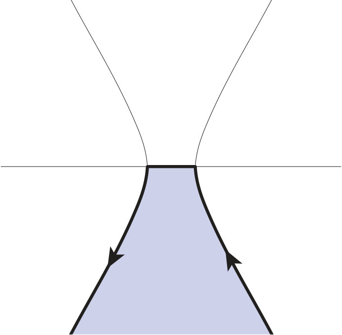 Figure 1
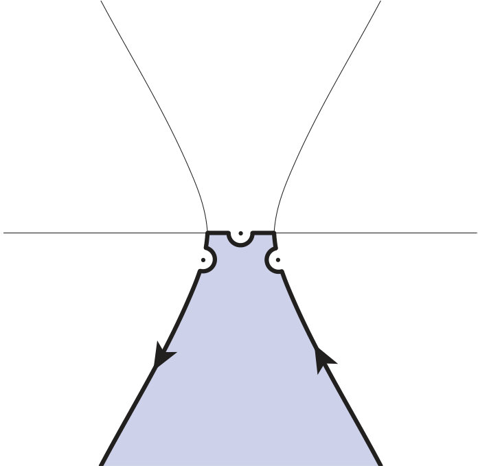 Figure 2
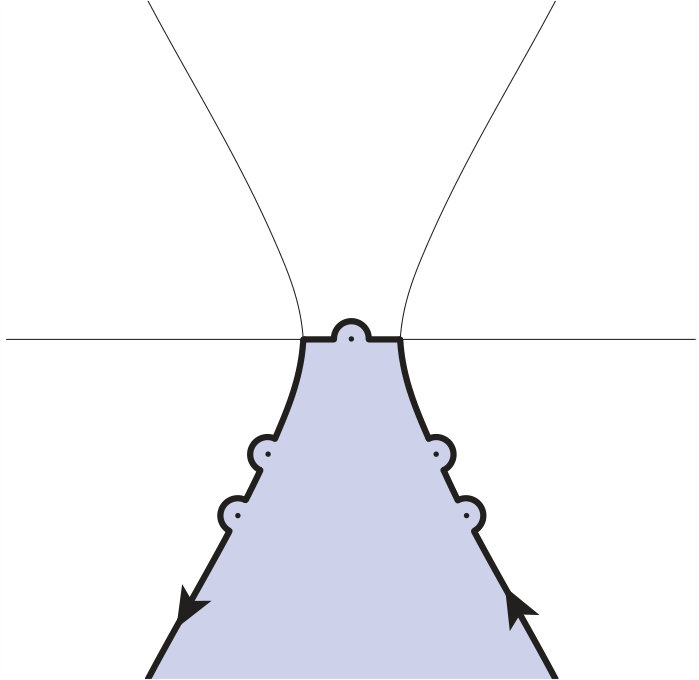 Figure 3
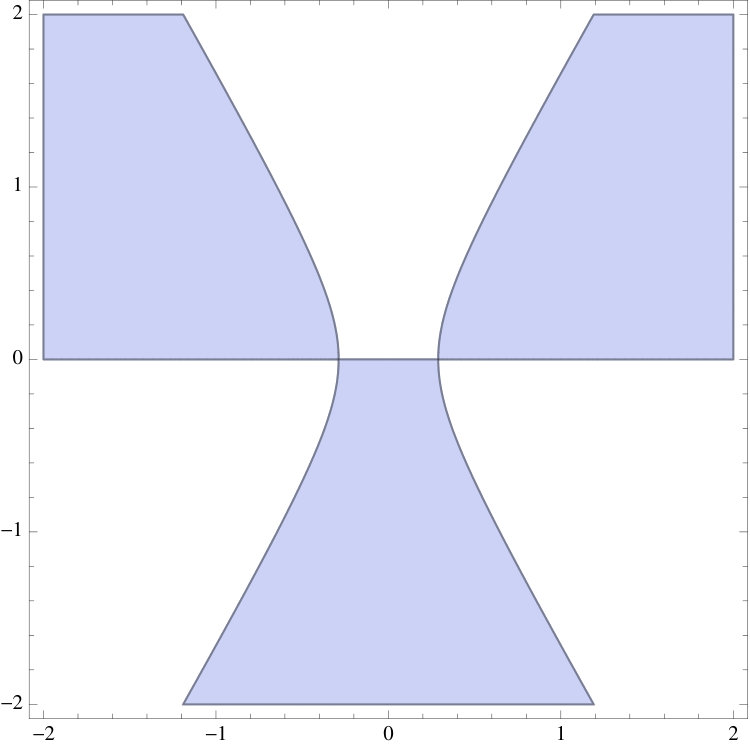 Figure 4
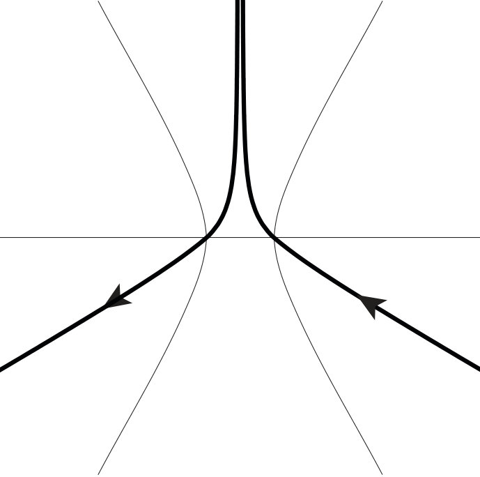 Figure 5
 Figure 6
Peer Reviews
No public reviews on file for this paper yet. If you reviewed it on a platform where reviews are public (OpenReview, ICLR, NeurIPS, ICML), you can paste yours below so the community can read it here.
Videos
No videos yet. Explain this paper in a talk, walkthrough, or lecture? Add one.
The KdV equation on the half-line:
Time-periodicity and mass transport
Jerry L. Bona
J.L.B.: Department of Mathematics, Statistics and Computer Science, University of Illinois at Chicago, 851 S. Morgan Street MC 249, Chicago, Il 60607, USA.
and
Jonatan Lenells
J.L.: Department of Mathematics, KTH Royal Institute of Technology, Stockholm, Sweden
Abstract.
The work presented here emanates from questions arising from experimental observations of the propagation of surface water waves. The experiments in question featured a periodically moving wavemaker located at one end of a flume that generated unidirectional waves of relatively small amplitude and long wavelength when compared with the undisturbed depth. It was observed that the wave profile at any point down the channel very quickly became periodic in time with the same period as that of the wavemaker. One of the questions dealt with here is whether or not such a property holds for model equations for such waves. In the present discussion, this is examined in the context of the Korteweg-de Vries equation using the recently developed version of the inverse scattering theory for boundary value problems put forward by Fokas and his collaborators. It turns out that the Korteweg-de Vries equation does possess the properly that solutions at a fixed point down the channel have the property of asymptotic periodicity in time when forced periodically at the boundary. However, a more subtle issue to do with conservation of mass fails to hold at the second order in a small parameter which is the typical wave amplitude divided by the undisturbed depth.
AMS Subject Classifications (2010): 35B30, 35C15, 35Q53, 37K10, 37K15, 76B15, 86-05.
Keywords: Water waves, initial-boundary-value problem, wave tank experiments, Korteweg-de Vries equation.
1. Introduction
The propagation of long-crested, unidirectional, small-amplitude, long wavelength disturbances over a featureless, flat bottom in shallow water can be approximately described by Korteweg-de Vries–type equations. A one-parameter class of such equations takes the form
[TABLE]
Here, the independent variable is proportional to distance in the direction of propagation while is proportional to elapsed time. The dependent variable is proportional to to the deviation of the free surface from its rest position at the point corresponding to at time . The real parameters
[TABLE]
are defined in terms of a typical amplitude and wavelength as well as the undisturbed depth of the water. The variables are scaled so that and its partial derivatives are formally all of order one while and are assumed to be small compared to one. The parameter is a modeling parameter that in principle can take any real value. However, the initial-value problem for the model will not be well posed unless .
In a flat-bottomed, laboratory channel, Zabusky and Galvin [31] ran experiments showing qualitative agreement between measurements and the model’s predictions for the case , the classical Korteweg-de Vries equation (KdV equation henceforth). Later work by Hammack and Segur [27] continued this line of investigation and also found qualitative agreement. The detailed accuracy of such models in the case , the BBM equation, was investigated in a series of wave tank experiments reported in [11]. In these experiments, a paddle-type wavemaker mounted at one end of the tank was oscillated periodically and the resulting wave motion was monitored at several points down the channel. More precisely, four measurements of the wave motion were taken at points . This produced four time series, and .
These measurements suggested an initial-boundary-value problem for (1.1) wherein the measurement was taken as boundary data for the equation and the initial data was identically zero, corresponding to the water being initially at rest. The predictions of this initial-boundary-value problem were then compared directly to the other three time series. As the equation (1.1) is an approximation for waves moving only to the right, the experiment ceases as soon as the waves reach the end of the channel and reflection becomes relevant. Hence, a natural boundary condition at , the end of the tank, is and, in the case of the KdV equation, the second boundary condition is also required. However, since a lateral boundary condition at the end of the channel away from the wavemaker is irrelevant to the motion prior to the wave reaching it, it is mathematically easier to simply push the right-hand boundary to infinity. Rigorous justification of this procedure on the time scale where there is no motion at can be found in [7] and [8]. The outcome of the comparisons made in [11] is that the just-described initial-boundary-value problem works quantitatively quite well, even for rather large values of the Stokes’ number .
In the course of examining the results of the experiments just described, two qualitative features of the wave motion emerged. The goal of the present essay is to address rigorously these two aspects in the context of the KdV equation, .
A. Time-periodicity. The experimental data indicate that a periodically moving wavemaker gives rise to measurements and which are asymptotically time-periodic with the same period as that of the wavemaker. In other words, if the wave maker oscillates with period , then the functions and approach functions which are periodic in with period as . Indeed, in the experiments, this approach is seen to be very rapid.
B. **Mass transport. ** In the experimental set-up, the total mass of the water in the channel is evidently constant. As the wavemaker oscillates periodically, the net amount of water added to the region beyond the first measurement point oscillates accordingly. Thus the function is expected to settle down to periodic oscillations around zero for large values of .
The plan of the paper is to introduce the principal theorems for both the linear problem in which the nonlinearity is dropped and the nonlinear problem in the next section. This will include a discussion of previous work on these problems. Theorem 2.1 will be proved in Section 3 while the nonlinear Theorem 2.2 and the resulting Corollary 2.3 will be dealt with in Section 4. The proofs are inspired by the developments in [25] where the nonlinear Schrödinger equation with asymptotically time-periodic data was considered. As mentioned, attention will be given only to the Korteweg-de Vries equation, the case . This is because the main tool used in the present investigation is inverse scattering theory. As far as we know, the model (1.1) does not have an inverse scattering theory if . A brief concluding section includes not only a summary of the results, but brief remarks on the implications for wave tank experiments.
2. Main results
In this section, the two principal results of our study are stated and discussed. The proofs are presented in Sections 3 and 4. An elementary rescaling of the independent and dependent variables assures that we may take and in (1.1). However, it must be remembered that the resulting boundary data now depends upon the parameters and .
The mathematical problem under consideration is then the equation
[TABLE]
together with the initial and boundary conditions
[TABLE]
where the given Dirichlet boundary value is taken to be smooth and compatible with the vanishing initial data at , which is to say . This initial-boundary value problem has received considerable attention. It is known to be globally well posed in a variety of circumstances to do with restrictions on the initial and boundary data (these development started with [16] and [17]; see [15] and the references contained therein for a more up-to-date appraisal). As the present discussion derives directly from experimental results, we are not going to be specially concerned with sharp hypotheses on the data. The answers to the issues just mentioned are the focus. Also, while the Korteweg-de Vries equation is known rigorously to approximate well solutions of the full, inviscid water wave problem (see [1], [10], [12], [21]), that fact depends upon smoothness of the auxiliary data. Without sufficient smoothness, there is no approximation.
2.1. The linear limit
The first theorem answers the questions posed in the introduction in the affirmative in the case of the linearized version of equation (2.1).
Theorem 2.1**.**
Let be a sufficiently smooth solution of the linearized KdV equation
[TABLE]
with vanishing initial data and compatible, periodic Dirichlet data of period , i.e.,
[TABLE]
For any fixed , is asymptotically time-periodic with period . More precisely, for each and as ,
[TABLE] 2.
For any fixed , the mass function has the property that as ,
[TABLE]
In particular, if has zero average, then is asymptotically time-periodic with period .
Asymptotic periodicity is established for the linear problem for both the KdV and the BBM equation in [18]. These results are obtained by classical energy estimates. The theory reported there is not as sharp as that obtained here using inverse scattering techniques. In any case, the linear inverse scattering theory is needed for our analysis of the nonlinear problem.
2.2. The nonlinear problem
In the second theorem, nonlinear corrections to Theorem 2.1 are kept and estimated. Thus, consider a perturbative solution
[TABLE]
of (2.1) with Dirichlet data
[TABLE]
where is a small parameter. The first and second Neumann boundary values of the solution are
[TABLE]
Their respective perturbative expansions are written as
[TABLE]
For definiteness, the results are presented when the Dirichlet data comprise a periodic sine-wave. Similar results can be obtained for other periodic boundary forcings. It is worth mentioning that the measured boundary conditions in the experiments reported in [11] closely resemble a sine wave while the boundary conditions used in the sediment transport study [3] were modeled exactly as sine waves with the field measured amplitudes and frequencies.
Theorem 2.2**.**
Let be a non-zero constant such that
[TABLE]
Let be a solution of (2.1) with boundary data
[TABLE]
Let denote the unique solutions of the cubic equations
[TABLE]
such that and belong to the boundary of the domain defined by
[TABLE]
(see Figure 1). Then, the first and second Neumann boundary values of at are as in (2.6), where, as ,
[TABLE]
Theorem 2.2 reveals that, at least to second order in perturbation theory, the time-periodic Dirichlet profile gives rise to time-periodic Neumann conditions. This suggests that the time-periodic Dirichlet data also generates a time-periodic solution in the nonlinear case.
Results of this nature for the nonlinear problem, but with damping incorporated, are discussed in [13]. That theory relies upon rather delicate Fourier analysis and is not as sharp as what is brought forth here.
The situation for mass transport is more complicated.
Corollary 2.3**.**
Under the assumptions of Theorem 2.2, the mass function satisfies
[TABLE]
where and, as ,
[TABLE]
*Proof. *Calculate as follows:
[TABLE]
It thus transpires that
[TABLE]
Since , the expressions for and obtained in Theorem 2.2 yield (2.10).
Equation (2.10b) implies that does not approach zero as . Indeed, if and only if
[TABLE]
and this equation is never satisfies for and . This suggests that a periodic Dirichlet boundary condition does not in general give rise to an asymptotically periodic mass function , although the discrepancy lies at second order.
3. Proof of Theorem 2.1
The first step is to derive an integral representation for the solution of the boundary value problem for the linear equation (2.3).
Define the open subsets of the complex -plane by
[TABLE]
Let where and . Similarly, let with and ; see again Figure 1.
For each , the cubic polynomial
[TABLE]
vanishes at exactly one point in each of the three sets , , and . Denote these points by , , and , respectively.
Lemma 3.1**.**
The solution for the initial-boundary-value problem (2.2) for the linearized KdV equation (2.3) has the representation
[TABLE]
in terms of the initial data and the Dirichlet data . Here, and
[TABLE]
*Proof. *Equation (2.3) is the compatibility condition of the Lax pair
[TABLE]
where is the spectral parameter and is a scalar-valued eigenfunction. Write (3.2) in differential form as
[TABLE]
where the closed one-form is defined by
[TABLE]
Stokes’ Theorem implies that the integral of around the boundary of the domain in the -plane vanishes. This yields the global relation
[TABLE]
where
[TABLE]
Multiplying equation (3.3) by and integrating the result along with respect to , it transpires that
[TABLE]
where Jordan’s lemma has been used to deform the contour from to in the second integral.
The final step consists of using the global relation to eliminate the two unknown functions and from (3.4). Letting , , in (3.3) gives
[TABLE]
Solving these two equations for and leads to
[TABLE]
Substituting these expressions into the solution formula (3.4) and observing that, Jordan’s lemma implies that the contributions from the terms involving vanish leads immediately to (3.1).
Now suppose that and that is periodic with period . To prove , note that equation (3.1) implies
[TABLE]
Making the change of variables in the part of the first -integral that runs along and using the periodicity of , there obtains
[TABLE]
Deforming the contour of integration from to the steepest descent contour , defined in Appendix A, and see also Figure 4, a steepest descent argument yields (2.4) (see Proposition A.1).
To prove , define by
[TABLE]
Equation (3.1) implies that
[TABLE]
where denotes the contour deformed so that it passes to the right of the removable singularity at .
Since the contour has been deformed to , the -integral can be split and the part involving can be calculated using Cauchy’s theorem to reach the formula
[TABLE]
Substituting this expression for into (3.6) gives
[TABLE]
Integrating by parts with respect to and using the periodicity of , it is inferred that the curly bracket in (3.7) equals
[TABLE]
Hence, for any and ,
[TABLE]
Deforming the contour of integration in the -integral from to , a steepest descent argument provides (2.5) (see again Appendix A and Figure 4).
4. Proof of Theorem 2.2
The proof relies on the formulas
[TABLE]
where as before and
[TABLE]
with
[TABLE]
These relations can be extracted from the nonlinear integral equations characterizing the Dirichlet to Neumann map of (2.1) derived in [28]. The roots satisfy the identities
[TABLE]
In consequence, it transpires that
[TABLE]
Furthermore, since
[TABLE]
Cauchy’s theorem implies
[TABLE]
For each integer , the third-order polynomial has three zeros; one zero in each of the three sets , and . Denote the unique solutions of in corresponding to and by and , respectively.
Several integrands will have singularities at points in the set . Let denote the contour depicted in Figure 3 with indentations inserted so that passes to the right of the points , and , Assumption (2.7) implies that these indentations can be chosen to lie in . Indeed, (2.7) implies that neither nor coincides with where . In fact, for , both and belong to the interval . For , and . For , . In particular, is a simple zero of and is a simple zero of . Similarly, is a simple zero of and is a simple zero of .
The discussion continues with the particular choice . Each of the expressions in (4.1) is considered in turn with this choice of boundary data.
4.1. Asymptotics of
Suppose . Equation (4.2a) becomes
[TABLE]
where
[TABLE]
Substituting this into (4.1a) and using Cauchy’s theorem gives the expression
[TABLE]
where the formulas
[TABLE]
have been applied. Using Jordan’s lemma to deform the contour to the steepest descent contour depicted in Figure 4, Proposition A.1 reveals that
[TABLE]
thereby establishing (2.8a).
4.2. Asymptotics of
Substituting (4.5) into (4.1b) and using Cauchy’s theorem provides the formula
[TABLE]
when . Here, we have used that
[TABLE]
Just as in the case of , a steepest descent argument shows that
[TABLE]
which proves (2.8b).
4.3. Asymptotics of
The computation of relies on (4.1c) and proceeds via a series of lemmas.
Lemma 4.1**.**
The integral in the last term on the right-hand side of (4.1c) is given by
[TABLE]
*Proof. *Equation (4.9) together with the identities
[TABLE]
imply that
[TABLE]
After substituting this expression into (4.4), formula (4.10) emerges.
Lemma 4.2**.**
The function in (4.2c) has the representation
[TABLE]
where and are given by
[TABLE]
and
[TABLE]
*Proof. *In view of (4.11), it transpires that
[TABLE]
Inserting this into the expression (4.3) for leads to
[TABLE]
where is as in (4.13). Computing the integrals with respect to gives (4.12).
Lemma 4.3**.**
The first term on the right-hand side of (4.1c) is
[TABLE]
*Proof. *This is a consequence of the expression (4.12) for and Cauchy’s theorem. For example, (4.12) implies that the coefficient of is
[TABLE]
Since the integrand has simple poles at and , Cauchy’s theorem implies that the latter integral equals
[TABLE]
Using (4.10) and (4.15) in the expression (4.1c) for , one finds that
[TABLE]
where
[TABLE]
To complete the proof of (2.8c), it is enough to show that is as . The proof of this fact is postponed to Section 4.5.
4.4. Asymptotics of
The computation of relies on (4.1d).
Lemma 4.4**.**
The last two terms on the right-hand side of (4.1d) can be written as
[TABLE]
*Proof. *This follows from the expression (4.7) for , the expression (4.10) for , and the fact that .
Lemma 4.5**.**
The first term on the right-hand side of (4.1d) is given by
[TABLE]
*Proof. *As in the proof of Lemma 4.3, this is a consequence of the expression (4.12) for and Cauchy’s theorem.
According to (4.1d), is the sum of the expressions in (4.18) and (4.19). Thus,
[TABLE]
where
[TABLE]
The proof of (2.8d) is completed by establishing that is in the next subsection.
4.5. Asymptotics of and
In this subsection, the proof of Theorem 2.2 is completed by showing that is of order as , .
Lemma 4.6**.**
The functions and defined in (4.6) and (4.14) satisfy
[TABLE]
and
[TABLE]
Proof.
A computation using (4.6), Proposition A.1, and Cauchy’s theorem shows that the left-hand side of (4.22) equals
[TABLE]
This proves (4.22). Recalling the definition (4.14) of and deforming the contour to , equation (4.23) follows immediately from Proposition A.1. ∎
Lemma 4.7**.**
The function defined in (4.13) satisfies
[TABLE]
*Proof. *First note that the definition (4.6) of and Cauchy’s theorem yield
[TABLE]
Substituting this and the expression (4.6) for into the definition (4.13) of and performing the integrals with respect to provides the formula
[TABLE]
To prove (4.25), multiply (4.26) by , , and integrate over . We claim that all the terms on the right-hand side of (4.26) which involve a factor of , , or are of order . Assuming for the moment that this is valid, it is inferred that the only contribution to , , derives from the last line of (4.26), which is to say,
[TABLE]
Computing the integral using the residue theorem, the asymptotic relations (4.25) emerge.
It remains to show that any term in (4.26) involving , , or yields a contribution of order O\big{(}t^{-\frac{3}{2}}\big{)}. This follows from steepest descent considerations. In Appendix B, the details of this calculation are provided for the case of the triple integral
[TABLE]
and the double integral
[TABLE]
The other terms can be treated similarly. The proof of Lemma 4.7 is complete.
Using equations (4.8), (4.22), (4.23), and (4.25) in the definitions (4.3) and (4.21) of and , respectively, there appears
[TABLE]
which completes the proof of Theorem 2.2.
5. Conclusion
Two questions about solutions of a natural initial-boundary-value problem for the Korteweg-de Vries equation have been addressed here. Both these questions arise naturally from observed experimental data obtained in water tank experiments. Overall, these results, which are asymptotic, but exact in their large-time structure, raise a cautionary note. While the positive result of asymptotic periodicity corresponds well to what is seen in experiments, the lack of asymptotically conserved mass is troubling. Admittedly, this does not occur at first order, in the notation in force here, but rather at the second order . As the Korteweg-de Vries model is only an accurate approximation on the so-called Boussinesq time scale of order , the fact that mass is not conserved at the higher order does not make the initial-boundary-value problem considered here necessarily suspect. However, it does reinforce the view that the model should not be pushed beyond the Boussinesq time scale. If a unidirectional initial-boundary-value problem valid on a longer time scale is needed, a higher-order correct model should be employed. A recent example of such a model is provided in [5] (and see the references therein to other, related models) and a relevant initial-boundary-value problem was put forward and analysed in [20]. However, this latter problem features a piece of boundary data that might be hard to obtain in a laboratory setting. This issue deserves further study.
Appendix A Steepest descent lemma
In this appendix, the method of steepest descent is used to determine the large behavior of certain integrals involving the exponential .
Let as before. The function vanishes at the two critical points . Let be the steepest descent contour shown in Figure 4. The contour is characterized by the condition that on the part of passing through , while on the part of passing through . For , let denote the part of that lies in the ’th quadrant. Then is strictly increasing from [math] to as moves away from towards along any of the ’s.
Proposition A.1**.**
Let be a function which is analytic in a neighborhood of . Suppose that grows at most algebraically as . It follows that
[TABLE]
*Proof. *Write the left-hand side of (A.1) as the sum , where denotes the contribution from , viz.
[TABLE]
Consider . For , let . The definition of the steepest descent contour implies that the mapping is a diffeomorphism from onto . Thus, a change of variables yields
[TABLE]
For any , the assumption that grows at most algebraically as implies that the integral
[TABLE]
is exponentially small. On the other hand, for near we have
[TABLE]
Thus, if has the expansion
[TABLE]
then
[TABLE]
Substituting this into (A.2) and evaluating the integrals with respect to leads to
[TABLE]
The last step can be made rigorous using standard arguments from the steepest descent method (see e.g. [29]). A similar argument applied to provides the asymptotic relation
[TABLE]
Equations (A.3) and (A.4) imply that .
Analogous computations give , thereby establishing Proposition (A.1).
Remark A.2**.**
The proof of Proposition A.1 can be extended to give the expansion of the integral in formula (A.1) to all orders in . In principle, a tedious computation can then provide the asymptotic expansions in (2.8) to all orders in .
Appendix B Asymptotics of and
Here, a proof is offered that and defined in (4.27)-(4.28) are also of order as .
Asymptotics of To prove that , note that the integrand in (4.27) has removable singularities at the points where . Moreover, the integrand is non-singular for in the set , so the contour in the -integral may be replaced with . Deforming the contour of integration in the -integral from to and interchanging the order of the and integrals, it is found that
[TABLE]
Next, deform the contour in the -integral so that it passes to the left (i.e. the indentation lies in ) of as well as to the left of the solutions in of the equations and (see Figure 5). Denote this deformed contour by .
For each pair , one observes that . In consequence, there exists a unique point such that
[TABLE]
Let denote the contour with a small indentation added so that it passes to the right of whenever . The following claim implies that this indentation can be chosen in such a way that for all .
Lemma B.1**.**
There exists an such that stays an -distance away from the critical points for .
*Proof. *Let denote the portion of that passes through . It will be shown that stays well away from for and . The case when can be handled in a similar way.
In view of (B.1), can approach only if is close to . Let be such that for . There exists a such that whenever satisfies . Thus, if is such that and , then by the triangle inequality,
[TABLE]
so that stays away from in this case. On the other hand, since for and is small only for near , there exists a such that whenever . Also, for . Hence, if is such that and , then
[TABLE]
showing that also stays away from in this case.
Since the contour avoids the point , it is the case that for all and . Hence, the integral may be split as follows:
[TABLE]
To compute , first use Jordan’s lemma to deform the contour to and then deform the contour in the -integral to infinity. Since implies , it follows that
[TABLE]
This implies that there exists a such that for all large . In particular, the integrand is as in . Thus, deforming the contour in the -integral to infinity, observing that has strictly negative real part and hence is nonzero throughout this deformation, it follows that .
To compute , remark that by deforming the contour to infinity and using Cauchy’s theorem, the formula
[TABLE]
emerges. The function vanishes at , but this singularity is removable since . In consequence, deforming the contour to infinity and using Cauchy’s theorem yields
[TABLE]
Since , the singularity at is removable. Deforming the contour to and applying Proposition A.1 yields , thereby showing that .
Asymptotics of To show that , notice that the integrand in (4.28) has removable singularities at the points where . To proceed, first deform the contour in the -integral from to and then deform the contour in the -integral from to . However, contrary to the earlier notation, the contour is now obtained from by inserting indentations so that it passes to the left of the origin and of the points at which (see again Figure 5). Since for and for with equality only at , can vanish only when and . In particular, for and . Thus the integral can be split, viz.
[TABLE]
To compute , observe that implies . It thus transpire that
[TABLE]
Thus, the integrand is as in . Deforming the contour in the -integral to infinity in , it follows that .
For the computation of , remark that
[TABLE]
Since , the singularity at is removable. Deforming the contour to and applying Proposition A.1, it is concluded that , thereby establishing that .
Appendix C An alternative perturbative approach
In Theorem 2.2 it was shown that if , then and are asymptotically periodic as , at least to second order in perturbation theory. We also computed the large asymptotics and gave rigorous error estimates for and to the same order.
If one assumes that and are asymptotically periodic as with period , and if one does not worry about precise error estimates, the coefficients in (2.8) can be determined directly using an alternative perturbative approach. This idea was first implemented for the nonlinear Schrödinger equation in [26].
The KdV equation (2.1) admits the Lax pair
[TABLE]
where is a vector-valued eigenfunction, is the spectral parameter, are defined by
[TABLE]
and denote the standard Pauli matrices. Letting and denote the first and second entries of respectively, the -part of (C.1) can be written as
[TABLE]
This in turn implies that the quotient satisfies the Ricatti equation
[TABLE]
Assume that the functions and are asymptotically time-periodic of period as . The functions to which they are asymptotic then have Fourier series representations
[TABLE]
Substituting these representations into equation (C.2) evaluated at leads directly to the equation
[TABLE]
This in turn yields the infinite hierarchy of equations
[TABLE]
C.1. Perturbative solution of the algebraic system
The algebraic system (C.4) may be solved perturbatively if the Fourier coefficients associated with the Dirichlet data are known. Indeed, a perturbative analysis of (C.4) yields expressions for the coefficients in terms of the , , and . The condition that be non-singular in then yields expressions for the Fourier coefficients and associated with the Neumann values in terms of the . This provides a straightforward, constructive approach to the Dirichlet to Neumann map.
In more detail, first substitute the expansions
[TABLE]
into (C.4). The terms of lead to the formulas
[TABLE]
For , let , , and denote the three roots of , ordered so that
[TABLE]
These roots satisfy the identities
[TABLE]
For to be nonsingular at and , it is required that
[TABLE]
Solving these equations for and using (C.6), there appears the formulas
[TABLE]
The equations (C.5) thus lead to
[TABLE]
Similarly, the terms of give
[TABLE]
The condition that should not have singularities at and determines the coefficients and . This process can be continued indefinitely. Indeed, the terms of order yield an equation of the form
[TABLE]
where the function is given in terms of (known) lower order terms. The condition that should not have singularities at and then implies that
[TABLE]
Once , , are determined, one may proceed to the next order.
Example C.1**.**
Consider the example wherein
[TABLE]
with satisfying (2.7). Then for all and
[TABLE]
As in Theorem 2.2, write and for and respectively. Equations (C.7) and (C.8) provide the formulas
[TABLE]
whence
[TABLE]
Thus, apart from the error terms, the expressions in (2.8a) and (2.8b) have been recovered.
Similarly, equation (C.9) yields
[TABLE]
For to not have singularities at and , it must be the case that
[TABLE]
Solving for and leads to
[TABLE]
Substituting in (C.10) and using the identities
[TABLE]
we find after some algebraic manipulations that
[TABLE]
For to not have singularities at and , it is required that
[TABLE]
which implies that . Similar considerations yield
[TABLE]
and
[TABLE]
Apart from the error terms, this recovers the expansions in (2.8c) and (2.8d).
Acknowledgement The gestation of this project took place when the authors were both participating in a conference held at the Schrödinger Institute in Vienna. The authors are especially grateful to the American Institute of Mathematics for providing an excellent environment for discussions during a weeklong National Science Foundation USA supported workshop on boundary-value problems for nonlinear, dispersive equations. JL thanks the University of Illinois at Chicago for support during a visit there and also acknowledges support from the European Research Council, Grant Agreement No. 682537, the Swedish Research Council, Grant No. 2015-05430, the Göran Gustafsson Foundation, and the EPSRC, UK. JB is grateful to Southern University of Science and Technology in Shenzhen for providing support for a visit there in the course of which the manuscript was finalized.
The reference list from the paper itself. Each links out to its DOI / PubMed record.
- 1[1] A. A. Alazman, J. P. Albert, J. L. Bona, M. Chen, and J. Wu, Comparisons between the BBM equation and a Boussinesq system. Adv. Differ. Equations 11 (2006) 121-166.
- 2[2] T. B. Benjamin, J. L. Bona and J. J. Mahony, Model equations for long waves in nonlinear, dispersive media. Philos. Trans. Royal Soc. London, Series A 272 (1972) 47-78.
- 3[3] B. Boczar-Karakiewicz, J. L. Bona, W. Romanczyk and E.G. Thornton, Modeling the dynamics of the bar system at Duck, NC, USA. In Proceedings of the 26th International Conference on Coastal Engineering (held in Copenhagen) 1998, American Soc. Civil Engineers: New York, pp. 2877-2887.
- 4[4] J. L. Bona and P. J. Bryant, A mathematical model for long waves generated by a wavemaker. Proc. Cambridge Philos. Soc. 73 (1973) 391-405..
- 5[5] J. L. Bona, X. Carvajal, M. Panthee and M. Scialom, Higher order models for unidirectional water waves. J. Nonlinear Science 28 (2018) 543-577.
- 6[6] J. L. Bona, S.-M. Sun and B.-Y. Zhang,
- 7[7] J. L. Bona, H. Chen, S.-M. Sun and B.-Y. Zhang, Comparison of quarter-plane and two-point boundary value problems: the BBM equation. Discrete Cont. Dynamical Systems, Series A 13 (2005) 921-940.
- 8[8] J. L. Bona, H. Chen, S.-M. Sun and B.-Y. Zhang, Comparison of quarter-plane and two-point boundary value problems: The Kd V equation. Discrete Cont. Dynamical Systems, Series B 7 (2007) 465–495.