Crystal Volumes and Monopole Dynamics
Sergey Cherkis, Rebekah Cross

TL;DR
This paper explores the dynamics of doubly periodic monopoles by relating their moduli space's Kähler potential to geometric volumes in Euclidean space, providing insights into their structure and behavior.
Contribution
It establishes a novel connection between the Kähler potential of monopole moduli space and Euclidean volume calculations, advancing understanding of monopole wall dynamics.
Findings
Derived a relation between Kähler potential and Euclidean volume.
Characterized the moduli space as hyperkähler and non-compact.
Linked monopole dynamics to geometric volume regions.
Abstract
The low velocity dynamic of a doubly periodic monopole, also called a monopole wall or monowall for short, is described by geodesic motion on its moduli space. This moduli space is hyperkaehler and non-compact. We establish a relation between the Kaehler potential of this moduli space and the volume of a region in Euclidean three-space cut out by a plane arrangement associated with each monowall.
Click any figure to enlarge with its caption.
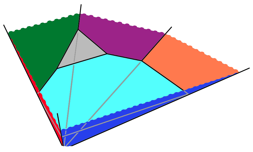 Figure 1
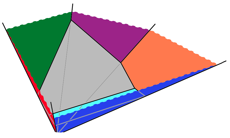 Figure 2
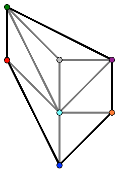 Figure 3
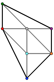 Figure 4
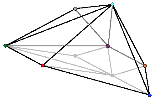 Figure 5
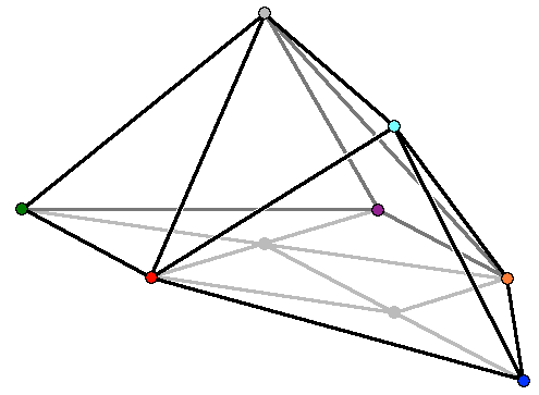 Figure 6
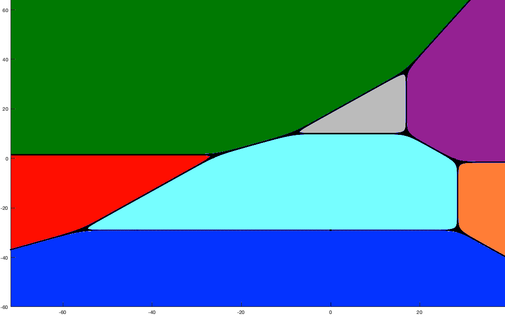 Figure 7
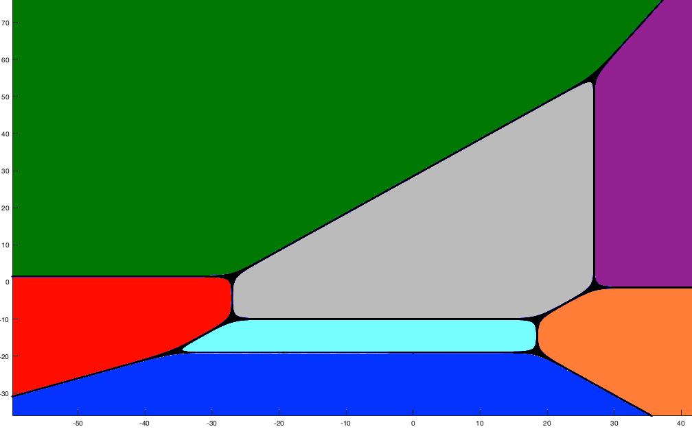 Figure 8
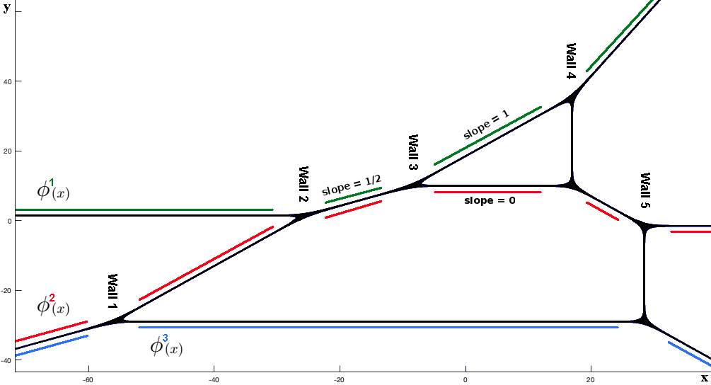 Figure 9
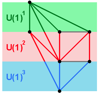 Figure 10
Peer Reviews
No public reviews on file for this paper yet. If you reviewed it on a platform where reviews are public (OpenReview, ICLR, NeurIPS, ICML), you can paste yours below so the community can read it here.
Videos
No videos yet. Explain this paper in a talk, walkthrough, or lecture? Add one.
Crystal Volumes and Monopole Dynamics
Sergey A. Cherkis
Department of Mathematics, University of Arizona, Tucson, AZ 85721 [email protected]
Rebekah Cross
Contents
1 Introduction
A monopole wall or a monowall is a BPS monopole on The latter space is endowed with coordinates and the product Euclidean metric with respective circle radii and , i.e. and In detail, a monowall is a Hermitian bundle of rank with a pair consisting of a connection on and a Higgs field , which is an endomorphism of satisfying the Bogomolny equation
[TABLE]
Here is the curvature of the connection (so in a local trivialization the curvature two-form is where is the connection one-form), is the Hodge star operator, and the covariant differential.
We impose the same asymptotic condition as in [CW12], namely that the eigenvalues of the Higgs field grow at most linearly, having the form
[TABLE]
as and the connection one-form has the form
[TABLE]
Here See [CW12, Sec.4] for the detailed discussion of charges , consistency conditions, and field asymptotics.
As argued in [CW12], it is natural to enlarge the scope of our problem by allowing for Dirac-type monopole singularities at some points and in At these points the Higgs field has (up to unitary gauge transformation) a prescribed singularity
[TABLE]
The first study of monopole walls, that we are aware of, was undertaken by Ki-Myeong Lee in [Lee99], where the deformation theory of monopole walls with arbitrary compact simple Lie gauge group was studied. The numerical study by Richard Ward of an monowall appeared in [War07] and [War11]. The spectral curve was used in [CW12] to study the deformation theory of monowalls. Hamanaka et al [HKM14] used monowall scattering to compute the moduli space asymptotic metric for monowalls. The interior of these moduli spaces was probed by Maldonado and Ward in [MW14] via special geodesics. A systematic description of the asymptotic region of the monowall moduli space and classification of the monowall moduli spaces of real dimension four appeared in [Che14]. For a general monopole, the asymptotic moduli space metric in the regime of widely separated constituents was found in [Cro15]. Monowalls relate to a number of significant problems involving non-abelian Hodge theory [Moc19], mirror symmetry [TWZ18], Calabi-Yau moduli spaces and quantum gauge theories in five dimensions [Che14, CDZS19], and integrable systems [Sci17].
1.1 Spectral Data of a Monowall
The Bogomolny equation (1) implies the compatibility of the following linear system
[TABLE]
Here is the covariant derivative along the -direction, etc. It follows that the holonomy around the -direction has eigenvalues that are meromorphic in the complex coordinate
[TABLE]
This motivates introducing the holomorphic spectral curve
[TABLE]
Moreover, the asymptotic conditions (2) and prescribed Dirac singularity conditions (3) ensure that this spectral curve is algebraic, given by , with the spectral polynomial
[TABLE]
Here is the lowest degree common multiple of the denominators of the rational functions appearing as coefficients of the characteristic polynomial This defines up to an overall constant nonzero factor. This ambiguity can be fixed, if desired, by imposing the dictionary order on the vertices and requiring the coefficient for the minimal vertex to be one. The Newton polygon is the minimal convex hull of all the points for which . The height of is equal to the monopole bundle rank
Note that our preferential treatment of the coordinate leading to the definition of the spectral curve was somewhat arbitrary. One can instead consider the modified holonomy around the direction and obtain a different spectral curve now covering the factor with coordinate .
Let Per denote the set of integer perimeter points of and let Int denote the set of its integer interior points. As demonstrated in [CW12], the Newton polygon is entirely determined by the charge values and the numbers of singularities and while the perimeter coefficients with are determined by the constants and appearing in the asymptotic conditions (and by the -coordinates of the Dirac singularities ). See [CW12] for details. The interior coefficients, on the other hand, are some of the moduli (parameterizing the deformations) of the monopole solution, thus producing a family of curves (with fixed perimeter coefficients). In fact, the total number of real moduli of a monowall is equal to four times the number of internal points: and the moduli space is the universal Jacobian fibration of this family
We shall focus on the region in the moduli space with large and large differences between them (as specified in Section 2 using the secondary fan). The generic curve for a family is a punctured Riemann surface of genus with punctures. Since, for any given monowall, is a curve of eigenvalues it (generically) comes equipped with a Hermitian eigen-line bundle with a flat connection . The triplet is the spectral data encoding the monowall solution up to a gauge transformation, with its parameters and moduli correspondence as follows:
- •
The holonomy of around each puncture is valued in and is determined by the asymptotic conditions. This is how the triplets of parameters of the boundary conditions translate to the spectral data [CW12, Sec. 4]: determine the position of each puncture, while determines the holonomy around it.
- •
Viewing a (generic) curve as a sphere with handles, one can associate each handle to an internal point of and choose a symplectic homology basis of the compactified Riemann surface with each pair associated to the -th handle. Thus, each internal point has four moduli associated to it: two real moduli and in and two moduli and specifying the holonomies and of around the cycles and respectively.
Let us emphasize an important distinction between parameters and moduli. Variations of moduli correspond to deformations of the solution of the Bogomolny equation (1), while variations of parameters result in deformations of the solution that are not square integrable. Physically, moduli correspond to all directions in the space of (gauge equivalence classes of) solutions that have finite mass, while the parameters are the remaining transverse coordinates. As a result, a monowall can slowly evolve in time with moduli changing, while all parameters will have to remain fixed, since their time evolution would require infinite energy. In other words the space of all monowalls with the given Newton polygon is fibered over the parameter space. The base is parameterized by the parameters and the fiber is what we call the moduli space. The coordinates on the moduli space are the moduli. The norm on the tangent space of pairs induces the metric on each moduli space.
1.2 The Crystal
Given a monowall and its spectral polynomial with coefficients , set and consider the set of planes
[TABLE]
Let us call the convex domain above all of these planes the cut crystal:
[TABLE]
Its surface is the graph of the function
[TABLE]
The shape of the cut crystal depends on the moduli (and parameters) and we shall be interested in how its volume changes with the change in the moduli Since the cut crystal has infinite volume, to keep track of these changes, let us also consider the domain above all of the perimeter planes only:
[TABLE]
Call it the the blocked crystal. Its surface is the graph of the function
[TABLE]
It is completely determined by the asymptotic conditions and is independent of the moduli, and it satisfies Thus, clearly, and the planes corresponding to the interior points of cut out of the blocked crystal .
We call the volume of the difference of the two crystals and the cut volume
[TABLE]
It is a function of variables , one for each integer point of
Intuitively, for large moduli a monowall would split into subwalls, as demonstrated in [Cro19]. As argued in Section 2, the subwall positions are well approximated by the positions of the vertices of this cut crystal. It was conjectured in [Che14] that the Kähler potential of a monowall moduli space is related to this cut volume (12). This paper refines this conjecture and proves it. This is based on the asymptotic metric found in [Cro15], obtained by analyzing subwall dynamic interactions via the Gibbons-Manton approach [GM95], reviewed in Sections 3. This metric approximates the metric on the moduli space end with exponential accuracy. The Kähler potential of this asymptotic metric is presented in Section 4. This Kähler potential, in turn, is the Generalized Legendre Transform (GLT) of Lindström and Roček [LR88, HKLR87] of the function The main result of this paper is that the GLT function encoding the asymptotic monowall metric equals the cut volume:
[TABLE]
The exact meaning and the proof of this relation are spelled out in Section 5. It can be summarized as follows:
in the regime of far separated subwalls the monowall Kähler potential is the Generalized Legendre Transform of the cut volume.
2 Subwall Positions and Spectral Curve Branch Points
As monowall moduli increase, the monowall splits into subwalls. Let us explore the dependence of these subwall positions on the moduli.
2.1 The Secondary Fan and the Monowall Spine
There is significant information about the monowall contained in the cut crystal. Its surface consists of
faces (each face contained in one of the planes (8) and thus each has an associated integer point ), 2. 2.
edges at which these faces meet, and 3. 3.
vertices.
The projection of the cut crystal edges and vertices on the plane is a graph, that we call the spine, as illustrated in Figure 1. From this description the spine is dual to a regular subdivision [GKZ08, Chs. 6 and 7] of the Newton polygon in which the two integer points of are connected by an edge if and only if the corresponding faces of the cut crystal meet at a crystal edge. Each spine edge is normal to the correspoinding edge of the subdivision of
A regular subdivision is defined in the following way. Consider a real valued function on the integer points of and the convex hull in of the set of downward rays The part of this hull’s surface that is not vertical is a graph of a concave function over the interior of in Let us call it the tent function. It is piecewise linear, with corners at (some of the points) . The edges of this surface project onto giving a regular subdivision of (Note, in some of the literature, e.g. in [GKZ08] itself, such subdivisions are called coherent subdivisions instead of regular subdivisions.) In our case, choosing results in a subdivision dual to the monowall spine. Also, note that the resulting tent function is the negative of the Legendre transform of the cut crystal surface function of Eq.(10).
As a result, the space with coordinates is subdivided into cones labelled by regular subdivisions of These cones form the secondary fan of Moving to infinity within a given cone results in the monowall splitting into subwalls of certain types, determined by the elements of that corresponding subdivision. Each polygon appearing in the subdivision corresponds to a subwall.
The secondary fan is encoded in the secondary polytope In fact, the two are dual to each other: each ray of is normal to a face of and two rays are connected by a wedge if the corresponding faces of share an edge. The th coordinate of the vertex of can be read off from its corresponding regular triangulation as the total area of the triangles for which the th integer point of is a vertex. See [GKZ08] for many fascinating details.
There is a partial order on all regular subdivisions given by refinement. The maximally refined subdivisions are the regular triangulations with each triangle of area111As in [GKZ08], we normalize the area of a basic triangle with vertices and to be one, instead of a half. . This is the case we are most interested in here, as it corresponds to the monowall maximally split into elementary subwalls.
Each regular triangulation labels a cone (of maximal dimension) in the secondary fan (see [GKZ08, Ch.6]), with other regular subdivisions labelling its lower-dimensional cones. According to [Che14, Sec.5], the secondary fan is in the space with coordinates which include both moduli and parameters. A generic direction lies in the interior of a single cone of the secondary fan and corresponds to some regular triangulation. Fixing all parameters gives a slice of . The intersection of this slice with the secondary fan divides this slice into regions, some compact and some noncompact.
The ‘down-facing’ cones of the secondary fan correspond to triangulations not involving any internal points of as triangle vertices. (These form the associahedral face of the secondary polytope, its largest face.) The maximally refined triangulations described above correspond to ‘upward-facing’ cones. It is these latter that correspond to asymptotic directions in the monowall moduli space (the noncompact regions of the secondary cone subdivision of an slice). Such, regular triangulations describe generic asymptotics of a monowall moduli space.
To summarize, for a regular triangulation there is the following correspondence illustrated in Figure 1:
each face of the spine222A spine face is the projection of a face of the cut crystal. corresponds to an integer point in the Newton polygon 2. 2.
each edge of a spine is an interface between faces and and it is orthogonal to the edge of the triangulation connecting the two corresponding integer points and of and 3. 3.
each vertex of the spine corresponds to a triangle of the triangulation Triang of
Clearly, point 2. above can be stated as: the spine edge connecting vertices and is orthogonal to an edge of the triangulation of the Newton polygon that is shared by the triangles and
2.2 Subwall Positions
Let us now explore the generic asymptotic region in the monowall moduli space by fixing a regular maximal triangulation and moving along a ray in the corresponding upward facing cone of the secondary fan. Each triangle of this triangulation corresponds to a vertex of the spine. We claim that (up to a constant, moduli independent, shift) the position of this vertex is the position of the corresponding subwall into which the monowall splits. To be exact, we understand the position of the subwall to be the point of (partial) gauge symmetry restoration, i.e. the branch point of the spectral curve
2.2.1 Spine Vertex
Consider a triangle of the regular maximal triangulation. Say its vertices are and ordered counterclockwise. A crystal vertex corresponding to that triangle is positioned at the point satisfying
[TABLE]
with solution
[TABLE]
Since the triangulation is maximal and the points are numbered counterclockwise, the triangle has minimal area, thus the denominator in (15) is and the position of the spine vertex is To simplify the notation, let and and same for other quantities, then
[TABLE]
2.2.2 Spectral Curve Branch Points
The holonomy of breaks the gauge symmetry, and when the gauge symmetry is maximally broken to the Bogomolny equation for the resulting fields is Abelian, implying that the Higgs field is harmonic. Thus, at large distances the Higgs field is linear. Therefore, it is exactly the regions where the gauge symmetry is at least partially restored that can be viewed as the sources of electromagnetic fields. This argument (at least in the limit of large separation of all subwalls) associates the magnetic charge to the regions where some eigenvalues of the holonomy coincide. In other words, the monowall consists of subwalls positioned at the branch points of the spectral curve. These subwalls carry magnetic charges and the magnetic field is constant between them.
Our immediate task is finding the locations of the branch points, in particular, their coordinates, with and comparing them with the locations of the spine vertices found above. As moduli become large, so does the spectral curve. To keep the whole curve in view, we rescale the coordinates accordingly. To begin, let and We consider the relevant locations of the branch points as is sent to zero, which corresponds to the large moduli region.
From the basic Puiseux expansion, each branch point is governed by three relevant monomials of the spectral polynomial (see [Cro19] for details), corresponding to the vertices of some triangle of the given regular triangulation of , therefore we can focus on
[TABLE]
The other terms are exponentially small ( with some ) in the moduli. If needed, relabel the vertices so that Let and for If needed, exchange the indices and to have the counterclockwise orientation, so that Now, the above equation reads In the new variables and Eq.(19) becomes thus with and
In terms of and the original variables are
[TABLE]
Branching of as a function of can only occur at the branch points of the solution of (20). These occur at the roots of the discriminant of the polynomial
[TABLE]
The discriminant is proportional to the resultant , which we now compute.
Let us list some basic properties of the resultant (see e.g. [Swa62]) of a pair of polynomials:
[TABLE]
where , and
Clearly,
[TABLE]
And the resultant is
[TABLE]
It vanishes at
[TABLE]
This is the position of a branch point corresponding to the triangle . In terms of the spatial position of this branch point of the spectral curve, we have
[TABLE]
which matches the position of the vertex of the spine (16) up to terms. The coordinate of the branch point is read off as the imaginary part of (26):
[TABLE]
Thus, for large values of the subwalls are positioned at the locations of the vertices of the spine. Moreover, the and positions of the wall associated to the spine vertex (corresponding to the triangle of the triangulation) are expressed via the same relation
[TABLE]
where the sum is over the three spine faces containing to the vertex When these three faces are numbered counterclockwise, the coefficients are and
2.3 Subwall Charges and Inter-wall Fields
If the vertices of the spine indicate the subwall positions, the spine edges approximate the eigenvalues of the Higgs field between the walls (to exponential accuracy in distance to the nearest wall). Away from all subwalls the gauge symmetry is broken to with each factor associated to one holonomy eigenvalue . We order these eigenvalues in decreasing order of so that Thus, each is a continuous, piecewise linear function of with kinks at the spine vertices. Away from the walls we have Higgs field
[TABLE]
where is the distance to the closest wall and the constant is the characteristic wall width, computed in [Cro15, Sec.3].
Since each spine edge, orthogonal to the edge of the triangulation of , corresponds to of the ordered eigenvalues, now all non-vertical edges of the spine are labelled by the factor indices , as illustrated in Figure 3. If we associate each index value to some distinct color, then the spine consists of continuous lines going left to right, each piecewise linear with kinks at the spine vertices. Each colored line is a graph of a function . It corresponds to an (approximate) Higgs diagonal value and the slope of the line is the magnetic field of the corresponding factor. The difference in line slopes and across the wall is the magnetic charge in that th factor of the wall corresponding to this spine vertex.
Next, we interpret the resulting fields as a superposition of individual subwall contributions and explore the subwall dynamics.
3 Subwall Interactions
The moduli space of a monowall is of real dimension with half of the moduli being the coefficients (for ) of the spectral curve and the other half parameterizing the Hermitian eigen-line bundle with a flat connection over We view this moduli space as a three-torus fibration over the dimensional space with base coordinates and the fiber coordinates The space of ‘long’ moduli and parameters factors as a direct product of the space of all ‘long’ moduli and of the space all ‘long’ parameters. As we discussed, this space contains the secondary fan whose maximal cones are indexed by the regular triangulations of the Newton polygon The space of long moduli is obtained by fixing the values of the long parameters. This is the base space of the moduli space fibered by tori. It traverses this fan, and the fan subdivides it into polytopal regions, each region corresponding to a phase of the monowall. The monowall in each phase, labelled by a triangulation Triang is well approximated (for sufficiently large moduli) by an array of subwalls. And -th subwall corresponds to a triangle and it carries Abelian charges (defined by the slopes of the two sides of the triangle to which the graph of is associated). Away from any subwall the Higgs field is essentially diagonal with
[TABLE]
Here and and the subwalls’ positions are
Let us discuss the meaning of (31) in detail, neglecting the exponentially small terms from now on. A single Abelian wall positioned at produces fields and with
[TABLE]
The superposition of such fields has left-right symmetric asymptotics. To accommodate general monowall charges, let
[TABLE]
so that the total fields are
[TABLE]
Now, any variation of the moduli produces some motion of the subwalls. A moving charged wall produces Liénard-Wiechert potentials [Cro15, Eq.(16)], instead of those of the static potentials of Eq.(32). In addition, each wall has an associated electromagnetic phase. Time dependence of this phase produces an electric charge Thus, each subwall (with varying moduli) becomes a dyonic moving wall with magnetic charges , respective electric charges and velocity We spell out the explicit expressions for these potentials next.
3.1 Moving Dyonic Subwalls
To avoid superficial prefactors let and , so that for an Abelian monowall
[TABLE]
An elementary static wall positioned at produces
[TABLE]
where the one-form satisfies for example
[TABLE]
The superposition of such subwalls as in (35) produces the functions (31) read off from the spine with .
A BPS dyon with electric charge and magnetic charge satisfies BPS equations and [CPNS77], so an elementary dyonic wall can be described by the pentuple consisting of the scalar Higgs field , an electro-magnetic potential consisting of the time component function and a ‘vector’ component one-form and dual electromagnetic potentials (a function) and (a one-form). These are related by electromagnetic duality
[TABLE]
Here are the one-forms metric dual to the electric and magnetic vector fields, and are in the same relation as the electro-magnetic dual fields and
In these terms the fields of the th static dyonic wall with magnetic charges and electric charges positioned at are
[TABLE]
[TABLE]
The Lorentz boost (accompanied by the proper time delay) produced the Liénard-Wiechert potential produced by the moving dyonic wall. Our focus is on the dynamics of slowly moving walls, thus, we neglect terms higher than quadratic in the resulting Lagrangian. In particular, the typical time delay terms of the form can be safely replaced by The resulting fields are
[TABLE]
[TABLE]
Here and is the value of the one-form on the vector From now on we drop the higher order terms in and
A dyonic wall moves in the background of fields which are the sum of contributions of all other walls. For example, (keeping up to quadratic terms in and ) the Higgs field that the -th wall experiences is
[TABLE]
Similarly,
[TABLE]
Note, that since the fields produced by any given subwall itself vanish at its location, there are no self-interaction terms, and the sums above are extended over all walls. The resulting relativistic Lagrangian governing the -th subwall dynamics is
[TABLE]
with the background fields given by (3.1–54). This Lagrangian governing the motion of one of the subwalls should be understood as the part of the effective Lagrangian of the whole monowall governing the motion of all subwalls. In particular it is the part of that contains Note, that the two subwall interaction is symmetric, e.g. Thus, combining individual subwall Lagrangians into one333Each pairwise interaction contributes once. (and keeping terms up to quadratic in velocities and electric charges):
[TABLE]
with implicit summation over the repeated indices and and
[TABLE]
and
[TABLE]
3.2 Subwall Positions and Charges
3.2.1 Positions
As we discussed, the motion of the subwalls is highly choreographed, since the subwalls’ positions are dictated by the plane arrangement. Via Eqs. (16):
[TABLE]
where the sum is over the three faces that have as a their vertex and the coefficients are as in Sec. 2.2.1. In fact, the -position of the wall is determined by the same relation
[TABLE]
As mentioned in Sec. 1.1, one can consider another spectral curve . Analysis of its branch points leads to the same subwall position relation
[TABLE]
Next, we focus on understanding the relations between the electric charges of the subwalls. Namely, we shall now demonstrate that they also satisfy the same relation
[TABLE]
for independent variables , one for each internal spine face.
3.2.2 Electric Charges
Let denote the set of spine vertices, – the set of spine edges, and – the set of spine faces. We shall orient the edges rightwards (and up, if vertical). For an edge let denote its head and let denote its tail. Then the crystal vertex position is determined from the system of equations (14)
[TABLE]
satisfied for all faces for which is a vertex of :
Taking the difference of adjacent faces, one gets the spine vertex position from the equations
[TABLE]
for any edge beginning or ending at the vertex
Note that solutions of (66) are in one-to-one correspondence with solutions of (65). Also, Eqs. (66) describes a system of
- •
points in and
- •
lines in the same in , such that
- •
each point has three lines passing through it (corresponding to three edges for which is a vertex) and
- •
each line has two points on it (corresponding to the two ends of ).
The reciprocal view of the dual with coordinates gives the system of points and lines such that each point has two lines through it and each line has three points on it.
Note, that the whole system is completely determined by the set of distinct points , since (using the first configuration) each line is determined by two points on it.
Consider triplets with the (coincident) eigenvalue of at the wall where this eigenvalue has a kink. As earlier, we define for each spine edge Then, comparing the electric flux change across the subwall (LHS below) with the electric charge (RHS below), one has
[TABLE]
This was our very definition of the electric charge . This relation implies that is the same for any edge beginning or ending at .
This implies that for any edge Which in turn is equivalent to
[TABLE]
for any and any beginning or ending at .
Note, that (68) is also a system. In fact, since it has the same set of points it must be the same system of projective lines and points. Thus,
[TABLE]
We take the last equation as determining . The first equation, on the other hand, reads
[TABLE]
for any edge Since, and , we have and therefore the function on edges is potential on the dual graph, in other words, there is a function such that . Here denotes the spine face to the left of the oriented spine edge , and denotes the one to its right. Substituting this into Eq. (70),
[TABLE]
We conclude that the set of triples satisfies exactly the same system of equations as the triples with the role of played by Thus, are expressed via (16):
[TABLE]
and
3.3 The Asymptotic Metric on the Moduli Space
Now we are ready to read off the asymptotic metric on the moduli space within each maximal cone of the secondary fan. So far we can conclude that the effective Lagrangian (56), expressed in terms of the moduli and independent charges , is
[TABLE]
To lighten our notation from here on we denote by the matrix with entries and similarly for
The conserved charges should be viewed as momenta associated with the electromagnetic phase moduli In order to express the Lagrangian in terms of the moduli we perform the Legendre transform in
[TABLE]
This yields the effective Lagrangian:
[TABLE]
which describes free motion of a point on a manifold with the Pedersen-Poon [PP88] type metric
[TABLE]
This is the asymptotic metric on the moduli space of the monowall. Its terms are written in terms of the and of Eqs. (57-60) and the coefficients appearing in Eq. (29). Let us emphasize that each generic ray in the moduli space lies in a cone labelled by a regular triangulation of the Newton polygon. Thus, the end of the moduli space is divided into sectors, each with the corresponding asymptotic metric (77). The triangulation determines both the coefficients and the order of the subwalls’ positions
4 The Kähler Potential and the Generalized Legendre Transform
Consider approaching the infinity of the moduli space within some maximal cone of the secondary fan. Such a cone is specified by a triangulation Triang of the Newton polygon As we now demonstrate, the Kähler potential of the asymptotic metric is encoded in a single function:
[TABLE]
The relation is via the Generalized Legendre Transform of [LR88, HKLR87] as follows.
Number the subwalls from left to right, so that and introduce a Laurent polynomial in the auxiliary variable for each subwall
[TABLE]
and let
[TABLE]
Note, that thanks to (61 – 63) the polynomial coefficients associated to the positions of each wall are functions of the respective moduli (and parameters) :
[TABLE]
Consider the Generalized Legendre Transform of the following auxiliary function
[TABLE]
of the parameters and of three quarters of the moduli. Half of the complex moduli are The contour integration above is over a counterclockwise oriented small circle around zero. The remaining half of the moduli are related to the above coordinates by
[TABLE]
Importantly, constructed this way is guaranteed to satisfy the Laplace type system of equations
The Kähler potential is the Legendre transform of
[TABLE]
with on the right-hand side understood as functions of and determined by As usual for the Legendre transform and This gives , which is the negative inverse of the matrix Also as well as The resulting metric
[TABLE]
is directly expressed in terms of :
[TABLE]
which in terms of the real moduli and reads
[TABLE]
with the one-form The exact metric coefficients can be easily evaluated observing that
[TABLE]
and by direct calculation
[TABLE]
[TABLE]
Using one has
[TABLE]
which exactly matches Eqs. (57-60).
Thus, we directly verified that the resulting GLT metric (84) with (86) and (88) exactly matches the asymptotic metric (77) obtained from the subwall dynamics:
[TABLE]
5 From the GLT Function to the Cut Volume
5.1 Cut Volume
We make use of the Lawrence formula [Law91] for the volume of a simple convex polytope
[TABLE]
which is a sum of signed volumes of simplices with
[TABLE]
the signed volume of the simplex with its apex at and its base in the base plane Here
- •
is one of the vertices of with exactly of the planes passing through it,
- •
the corresponding simplex is cut out by these planes and the base plane with some fixed vector not normal to any of the polygon planes,
- •
the constants are the coefficients in the decomposition
[TABLE]
Let us gain some appreciation of this formula (91) by proving it. In dimension , let be the simplex edges emanating from its main vertex and ending on its base plane Let be a point in this base plane and let be its height, i.e. and Clearly the symplex volume is
[TABLE]
The corresponding vectors are normal to respective simplex faces, and thus each is proportional to the vector product of the two edges of that simplex face:
[TABLE]
To lighten our notation let By construction , thus
[TABLE]
giving Noting that we have the Lawrence formula take the form
[TABLE]
We used since is normal to the base plane continaining and
The signs in the Lawrence formula are chosen already so that the individual simplex volumes contribute with different signs and the polygon volume does not depend on the choice of the base plane
Let us choose a high horizontal plane for a very large value The cut volume is the difference of the volume of the (convex) regularized blocked crystal
[TABLE]
and the (convex) regularized cut crystal
[TABLE]
The Lawrence formula applies to both and and thus the cut volume is
[TABLE]
where the first sum is over the vertices at which three perimeter planes (i.e. planes corresponding to the points in Per) meet or at which two perimeter and one top plane meet. The last sum is over the vertices involving an internal plane as well as the vertices involving the top plane. The latter contributions cancel (as, indeed, the cut volume does not depend on the choice of the high top plane). The remaining contributions are moduli independent, thus, up to a constant, the volume we are interested in is
[TABLE]
with the apex of the cone cut out by for three internal points forming the triangle of the triangulation. In the Lawrence formula we choose and , and have Thus, , where is the area of the triangle444Here we use our conventions of the footnote on page 2, i.e. is twice the conventional triangle area. And the relevant factors read off from are . The resulting volume formula is
[TABLE]
with the triangle positively oriented.
5.2 GLT Function
The GLT function (78) is
[TABLE]
In terms of the Higgs field (35), this reads
[TABLE]
For any given subwall all factors which have a nonzero charge have the same value , while the charges themselves satisfy , since555We suppose for concreteness that of the factors have and of the factors have
[TABLE]
Thus, the first term in (102) vanishes. If we let denote the magnetic flux in the -th factor to the right of the -th subwall, then and , as defined in (34). Thus, the second term in (102) is a telescoping series: and , therefore, the last term becomes Summing over the factors, As a result
[TABLE]
Here is twice the conventional area of the triangle associated with -th subwall.
Comparing to (100) we conclude that the GLT function is equal to the cut volume:
[TABLE]
6 Outlook
The effective dynamics of a monopole wall are given by the electromagnetic interaction of its constituents. In the low speed approximation it produces the effective Lagrangian from which we read off the resulting asymptotic moduli space metric. We proved that the Kähler potential of this metric is the Generalized Legendre Transform of the regularized crystal volume cut out by the plane arrangement. The latter volume can be easily read off from the monopole charges, parameters, and moduli.
The remaining challenge is to find the Kähler potential for the whole moduli space. With this goal in mind we now pose some questions and take the liberty of making some speculations.
There is a more refined volume function at hand that could capture some of the Kähler potential subleading asymptotic behavior. Consider the Ronkin function
[TABLE]
It is linear outside of the amoeba with Note that as moduli approach infinity These planes lead to a function The region above the graph of is the melted crystal. One can consider the volume of the region and use this melted volume instead of the cut volume used in this paper. For large moduli these two volumes and are exponentially close to each other and thus produce the same asymptotic.
One might seek to combine the two Ronkin functions and , for example, incorporating both and spectral curves and to encode the complete Kähler potential.
The relation between the two Legendre transforms that we used can be summarized in the following diagram:
[TABLE]
This leads to a question: Is there a more direct relation between the tent function and the Kähler potential? Is there a natural physical meaning of the Legendre transform of the Ronkin function in this context?
Let us conclude with a conjecture for the auxiliary function for the exact Kähler potential. To begin, we define the Twistor Spectral curve [Che07] via the Hitchin scattering problem [Hit82]. The space of oriented lines in the covering space of the base space is the minitwistor space . Each line is determined by the unit vector of its direction , (which determines the point with the complex coordinate on the Riemann sphere ) and the line’s displacement from the origin (which is a point in the tangent plane at with coordinate ). For each line, consider the scattering problem For some lines this problem has an solutions. These lines are called the spectral lines. Each line in is a point in and the set of all spectral lines forms a curve in Since our initial problem is invariant under discrete shifts in the and directions, the curve descends to a curve in the quotient space which is the space of geodesics in Let be the local branches of this twistor spectral curve. We conjecture that
[TABLE]
produces the exact Kähler potential.
The challenge in using such a relation is that even for the conventional monopoles in the twistor curve is notoriously difficult to find, as it should satisfy a complicated ‘triviality condition’. In addition, for monowalls, the curve is contained in the minitwistor space that is non-Hausdorff, while its cover is of infinite genus. Some recent approaches, such as in [Moc19], provide promising perspectives on this problem.
Acknowledgments
SCh is grateful to the organizers of the 2019 workshop “Microlocal Methods in Analysis and Geometry” at CIRM–Luminy and to the Institute des Hautes Études Scientifiques, Bures-sur-Yvette where the final stages of this work were completed. SCh received funding from the European Research Council under the European Union Horizon 2020 Framework Programme (h2020) through the ERC Starting Grant QUASIFT (QUantum Algebraic Structures In Field Theories) nr. 677368. RC thanks the Marshall Foundation for her Dissertation Fellowship funding.
The reference list from the paper itself. Each links out to its DOI / PubMed record.
- 1[CDZS 19] Cyril Closset, Michele Del Zotto, and Vivek Saxena, Five-dimensional SCF Ts and Gauge Theory Phases: an M-theory/type IIA Perspective , Sci Post Phys. 6 (2019), 052, ar Xiv:1812.10451 , doi:10.21468/Sci Post Phys.6.5.052 . · doi ↗
- 2[Che 07] Sergey A. Cherkis, A Journey Between Two Curves , SIGMA 3 (2007), 043, ar Xiv:hep-th/0703108 , doi:10.3842/SIGMA.2007.043 . · doi ↗
- 3[Che 14] , Phases of Five-dimensional Theories, Monopole Walls, and Melting Crystals , JHEP 06 (2014), 027, ar Xiv:1402.7117 , doi:10.1007/JHEP 06(2014)027 . · doi ↗
- 4[CPNS 77] Sidney R. Coleman, Stephen J. Parke, Andre Neveu, and Charles M. Sommerfield, Can One Dent a Dyon? , Phys. Rev. D 15 (1977), 544, doi:10.1103/Phys Rev D.15.544 . · doi ↗
- 5[Cro 15] Rebekah Cross, Asymptotic Dynamics of Monopole Walls , Phys. Rev. D 92 (2015), no. 4, 045029, ar Xiv:1506.07606 , doi:10.1103/Phys Rev D.92.045029 . · doi ↗
- 6[Cro 19] , Doubly Periodic Monopole Dynamics and Crystal Volumes , Ph.D. thesis, University of Arizona, 2019.
- 7[CW 12] Sergey A. Cherkis and Richard S. Ward, Moduli of Monopole Walls and Amoebas , JHEP 05 (2012), 090, ar Xiv:1202.1294 , doi:10.1007/JHEP 05(2012)090 . · doi ↗
- 8[GKZ 08] Israel M. Gelfand, Mihkail M. Kapranov, and Andrey V. Zelevinsky, Discriminants, Resultants and Multidimensional Determinants , Modern Birkhäuser Classics, Birkhäuser Boston, Inc., Boston, MA, 2008, Reprint of the 1994 edition. MR 2394437