Clustering Degree-Corrected Stochastic Block Model with Outliers
Xin Qian, Yudong Chen, Andreea Minca

TL;DR
This paper introduces a convex-optimization clustering algorithm for degree-corrected stochastic block models that effectively handles outliers, achieving exact recovery and lower error rates in heterogeneous networks.
Contribution
It presents a novel convex-optimization method with penalization for clustering in the presence of outliers, improving accuracy over existing algorithms.
Findings
Achieves exact cluster recovery under mild conditions.
Performs well on networks with Pareto degree distributions.
Reduces error rates compared to prior methods.
Abstract
For the degree corrected stochastic block model in the presence of arbitrary or even adversarial outliers, we develop a convex-optimization-based clustering algorithm that includes a penalization term depending on the positive deviation of a node from the expected number of edges to other inliers. We prove that under mild conditions, this method achieves exact recovery of the underlying clusters. Our synthetic experiments show that our algorithm performs well on heterogeneous networks, and in particular those with Pareto degree distributions, for which outliers have a broad range of possible degrees that may enhance their adversarial power. We also demonstrate that our method allows for recovery with significantly lower error rates compared to existing algorithms.
Click any figure to enlarge with its caption.
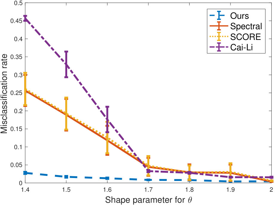 Figure 1
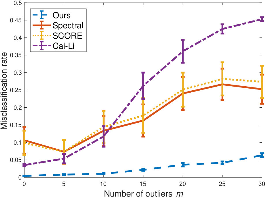 Figure 2
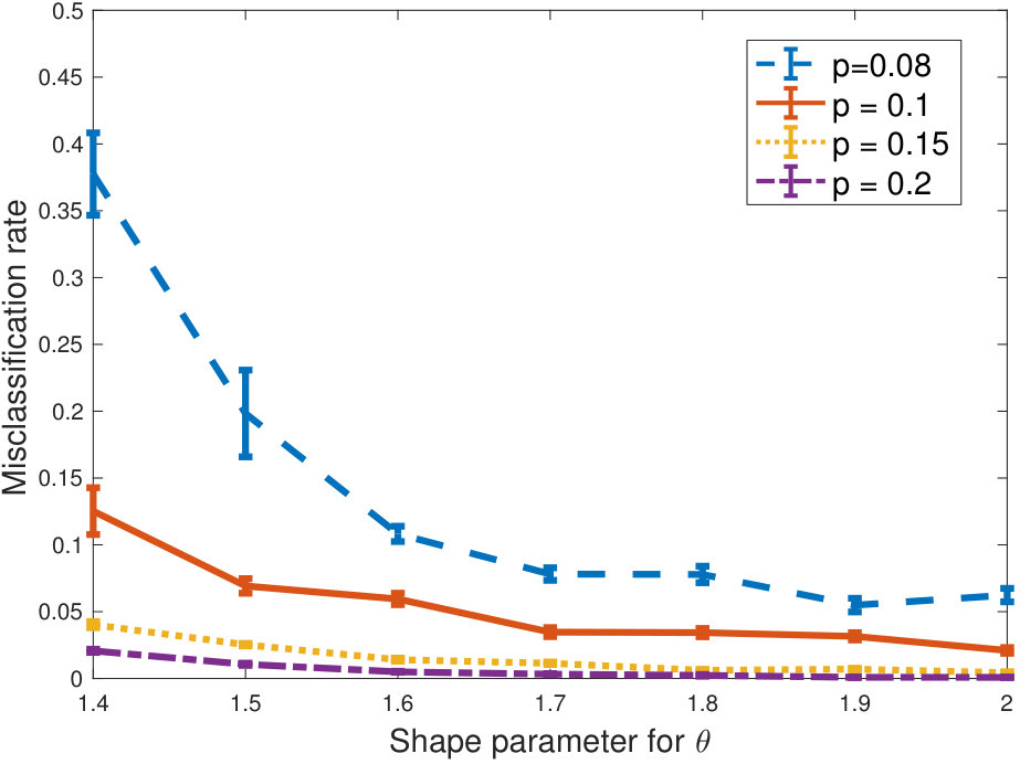 Figure 3
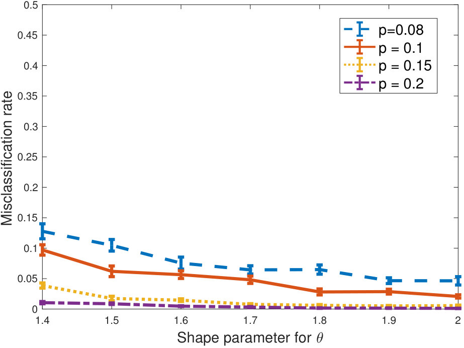 Figure 4
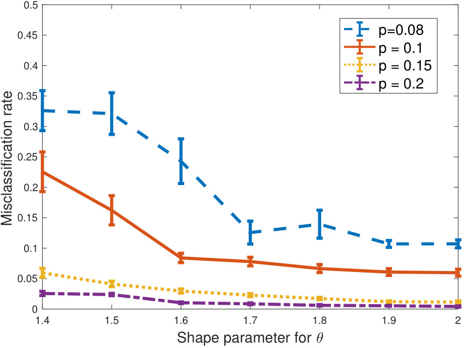 Figure 5
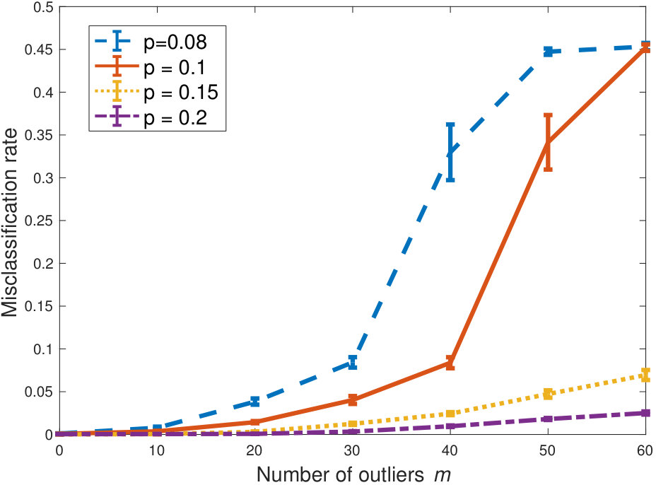 Figure 6
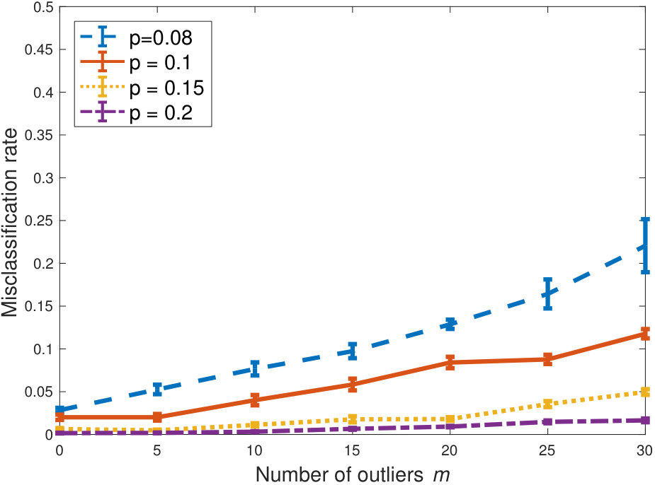 Figure 7
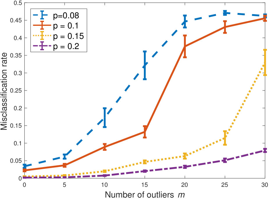 Figure 8
Peer Reviews
No public reviews on file for this paper yet. If you reviewed it on a platform where reviews are public (OpenReview, ICLR, NeurIPS, ICML), you can paste yours below so the community can read it here.
Videos
No videos yet. Explain this paper in a talk, walkthrough, or lecture? Add one.
Taxonomy
TopicsAnomaly Detection Techniques and Applications · Complex Network Analysis Techniques · Adversarial Robustness in Machine Learning
Clustering Degree-Corrected Stochastic Block Model with Outliers
Xin Qian Yudong Chen Andreea Minca Northwestern University, Industrial Engineering and Management Sciences, Ithaca, NY, 14850, USA, email: [email protected] University, School of Operations Research and Information Engineering, Ithaca, NY, 14850, USA, email: [email protected] University, School of Operations Research and Information Engineering, Ithaca, NY, 14850, USA, email: [email protected].
Abstract
For the degree corrected stochastic block model in the presence of arbitrary or even adversarial outliers, we develop a convex-optimization-based clustering algorithm that includes a penalization term depending on the positive deviation of a node from the expected number of edges to other inliers. We prove that under mild conditions, this method achieves exact recovery of the underlying clusters. Our synthetic experiments show that our algorithm performs well on heterogeneous networks, and in particular those with Pareto degree distributions, for which outliers have a broad range of possible degrees that may enhance their adversarial power. We also demonstrate that our method allows for recovery with significantly lower error rates compared to existing algorithms.
1 Introduction
Clustering nodes in a complex network is one of the major challenges in network science. Various aspects of this problem have been studied by researchers across different fields including computer science, statistics, operation research, probability and physics; for a partial list of work in this line, see Airoldi et al. (2008); Bickel and Chen (2009); Bordenave et al. (2018); Chen et al. (2014b); Clauset et al. (2004); Condon and Karp (2001); Dasgupta et al. (2004); Demaine et al. (2006); Fortunato and Barthelemy (2007); Fortunato (2010); Guédon and Vershynin (2015); Lei et al. (2015); Massoulié (2014); Newman and Girvan (2004); Nowicki and Snijders (2001); Rohe et al. (2011); Shamir and Tishby (2011); Yi et al. (2012); Zhang et al. (2014).
A variety of clustering algorithms have been developed, such as modularity maximization (Newman, 2006; Karrer and Newman, 2011), graph-cut based methods (Condon and Karp, 2001; Bollobás and Scott, 2004), model/likelihood-based methods (Zhao et al., 2012; Le et al., 2016), spectral clustering (McSherry, 2001; Shi and Malik, 2000; Ng et al., 2002), hierarchical clustering methods (Balcan and Gupta, 2010), and more recently algorithms for dynamic networks (Hajek and Sankagiri, 2018).
A main goal and driving force for the development of new algorithms is to tackle features of real world datasets, among those size and heterogeneity of the networks. In many cases, promising algorithms remain heuristic and are not yet amenable to rigorous performance analysis. On the theory side, obtaining provable performance guarantees is hindered by the fact that each realistic feature added to the network model significantly increases the complexity of the analysis.
A recent line of research on clustering makes use of convex optimization to achieve both computational efficiency and statistical quality guarantees (Chen et al., 2014a, b; Ames and Vavasis, 2011; Cai and Li, 2015; Guédon and Vershynin, 2015). By relaxing the original combinatorial problem into a semidefinite program (SDP), tractable clustering algorithms are developed which, under very general statistical settings, provably produce a high quality clustering. With a few exceptions such as Dasgupta et al. (2004); Karrer and Newman (2011); Chen et al. (2018), most previous work in this area considers homogeneous networks, in which different nodes exhibit similar statistical properties.
In this paper, we focus on designing clustering algorithms applicable to heterogeneous networks with outliers, and on providing theoretical guarantees for them. In particular, we would like to simultaneously capture the following three key features common in real world networks:
- •
Clustering/community structure: Nodes may belong to several different groups, where nodes in the same group are more likely to connect to each other than those in different groups.
- •
Heterogeneous degrees: It is well-documented that real-world networks have heterogeneous node degrees. In particular, the degrees of nodes, even those in the same cluster, may exhibit heavy-tailed distribution (Newman, 2010).
- •
Arbitrary outliers: There may exist a set of nodes that do not belong to any clusters and have arbitrary, even adversarial connection patterns.
Many networks have these properties. For example, the political blogs networks (Adamic and Glance, 2005) contain blogs that are mostly democratic or republican-oriented, some of whom have significantly more followers than others, but there are blogs that are associated with neither political groups. Another important example is given by financial networks. These consist of thousands of nodes at most but face a lot of heterogeneity. More importantly, the number of clusters is known and small. Clusters represent classical investment strategies, while some of the firms are multi-strategy and can be thought of as outliers (Guo et al., 2016). Arbitrary outliers could also correspond to non-bank firms connected in financial derivatives markets (Peltonen et al., 2014). Last and probably most important, for genomic networks, there are a variety of co-expression networks that suffer from the presence of outliers. For example, cancer-type-specific co-expression networks are medium sized network of 10-20 thousand genes and network analysis and clustering can be useful to identify prognostic genes for some types of cancer, Yang et al. (2014).
Note that the outliers may be different in nature among themselves, so one cannot simply treat them as an additional cluster and apply a standard clustering algorithm. Indeed, many existing methods, such as spectral clustering, are known to perform poorly in the presence of outliers even in small datasets (Cai and Li, 2015).
1.1 Our Contributions
Motivated by the considerations above, we consider a network model that accounts for the combined features. The clustering algorithm we consider is based on Semidefinite Programming (SDP) relaxation of the Modularity Maximization approach. We introduce a novel regularization term that penalizes outliers with unusual connection patterns beyond those implied by the inlier heterogeneity.
Two existing works serve as the foundation of our analysis: the Stochastic Block Model (SBM) with Outliers in Cai and Li (2015) and the Degree-Corrected Stochastic Block Model (DCSBM) in Chen et al. (2018). As usual, the complexities arising by adding multiple realistic features largely surpass complexities of handling any of these features alone. In particular, our analysis needs to address the following challenges:
(1) When inliers are homogeneous, a node with unusual degree can be immediately recognized as an outlier. Therefore, for an outlier to hide, it must have a degree that is similar to inliers’ degree. This limits significantly the power of the adversary. In real networks, however, a node with unusual degree may not be an outlier – it can well belong to one of the clusters, and have very high or low degree simply because this node is more popular/unpopular than other nodes in the same cluster. In this sense, we are facing the more challenging problem where the outliers have more freedom and do not need to restrict their degrees. The ability of the outliers to select across a broad range of degrees (especially when the inliers’ degree distribution is heavy-tailed) makes it crucial for an algorithm to look into the detailed connectivity patterns of the nodes (who connects to whom) rather than just their degrees (how many they connect to), even more so than SBM.
(2) We use the primal-dual witness approach. However, in proving the necessary bounds for the recovered solution, we need to bound separately the contributions from nodes with different degrees. The heterogeneous nature of the nodes’ connectivity complicates the analysis on the distribution of edges. We need to obtain sufficiently tight individual bounds and ensure the correct dependence on the individual degrees such that the aggregate bound is sufficiently strong. In contrast, a worse case bound in terms of the maximum degree would be too loose. Moreover, in the degree-corrected set-up, the definiteness of the adjacency matrix becomes worse and the homogeneous penalization on diagonal terms is not enough to recover the true clusters. We instead introduce a term that depends on the degree of each node, namely it takes the form , where is depends both on the degree vector and a control on the expected number of edges to other inliers.
By addressing these points, we provide theoretical guarantees for the exact recovery of the inlier nodes with high probability. In particular, we impose no assumptions on the outlier nodes other than their cardinality. We provide an explicit and non-asymptotic condition for exact recovery. Namely, we request that the density gap (difference between the intra- and inter-cluster edge density) must be larger than an expression based on the natural problem parameters, such edge densities, amount of degree heterogeneity, sizes of the clusters, and number of inliers/outliers. We also give explicit conditions on the tuning parameters of the algorithm. Surprisingly, the condition for recovery does not contain an “nm” term as in (Cai and Li, 2015) and instead contains two terms in “n” and respectively ””.
The applicability of our model is to networks of several thousands of nodes. These are medium sized networks, which may arise in various applications and are subject to the real-world features described above. We provide numerical results based on synthetic data for a network of size in the range to , divided into clusters and in the presence of a varying number of outliers, . The degrees are following a heavy-tailed Pareto distribution, with varying shape parameters. We compare the misclassification rate for our algorithm to state of the art algorithms, such as spectral clustering (Zhang et al., 2014), SCORE (Jin, 2015) and Cai-Li (Cai and Li, 2015). Our results significantly improve the quality of recovery. Notably, the performance of the algorithm is relatively unhindered even under very heterogeneous degree distributions and in the presence of a large number of outliers. In contrast, other algorithms have a sharp increase in the misclassification rate in such settings.
1.2 Notation
Matrices are denoted by bold capital letters, vectors by bold lower-case letters, and scalars by normal letter. The notation means the matrix is positive semidefinite (psd). For two matrices and of the same dimension, we denote their trace inner product by by , and we write if for all and . For an integer , let We use to denote the identity matrix, the matrix with all entries equal to 1, and the diagonal matrix whose -th diagonal entry is . We use notations like etc. to denote numerical constants independent of the other model parameters (in particular, the number of nodes ). Finally, for two quantities and that may depend on , we write if they are of the same order, that is, there exist numerical constant and such that .
2 Problem Setup
We consider a Degree-Corrected Stochastic Block Model with Outliers, which is a generative model for a random graph with underlying clustering structures.
In particular, the model involves a graph . Here is a set of vertices, where inliers are partitioned into unknown clusters , and the other nodes are outliers. The adjacency matrix , where if and only if nodes and are connected, are generated randomly as follows. Each pair of distinct inliers and are connected by an undirected edge with probability , independently of all others. Here the vector is referred to as the degree heterogeneity parameters of the nodes. The symmetric matrix is called the connectivity matrix of the clusters, and specifies the likelihood of connectivity of the inliers. The connections of the outliers among each other and to the inliers are arbitrary; they may depend on the underlying clusters and the realization of edges between the inliers, and may even be chosen adversarially.
Note that the above model is a generalization of several well-known models. When there are no outliers () and is uniform, the model reduces to the classical SBM (Holland et al., 1983). If but is allowed to vary across , it becomes the standard DCSBM (Dasgupta et al., 2004; Karrer and Newman, 2011). Finally, when but may be non-zero, it coincides with the setting considered in Cai and Li (2015), i.e., the SBM with outliers.
For future development, it is convenient to write the adjacency matrix in a block form according to the clustering structure
[TABLE]
where the block matrices above have the following interpretations:
- •
is a symmetric 0-1 matrix representing the connection within the outliers. Under our model, is arbitrary.
- •
is a 0-1 matrix representing the connection between inliers and outliers; in particular, is the adjacency matrix between the outliers and the -th inlier cluster. Under our model, is arbitrary.
- •
is a symmetric 0-1 matrix representing the connection between inliers. In particular, is the adjacency matrix between the -th and -th clusters. Under our model, each entry of is equal to 1 with probability , independently of all others.
- •
is an unknown permutation matrix, in which there is a single 1 in each row and column while all other entries are 0. Under this permutation, the nodes are ordered according to the underlying structure of clusters and outliers.
For each , we denote the size of the -th cluster by be . Note that . Let be the minimum size of the clusters. We also introduce the vector of node degrees , where .
For each candidate partition of the inliers into several clusters, we may associate it with a partition matrix , such that if and only if nodes and are assigned to the same cluster, with the convention that . Ideally, we would like to find a partition matrix of the form
[TABLE]
where denotes the -by- all-one matrix, and denotes arbitrary entries. In other words, we want to correctly recover the cluster structure within the inliers, where cluster assignment of the outliers may be arbitrary.
Given a single realization of the resulting random graph , our goal is to recover the true inlier clusters , that is, to recover a partition matrix in the form of (2.2).
3 Algorithm: A Convex Relaxation Approach
In this section, we provide the motivation and description of our algorithm, which can handle both degree heterogeneity and outliers.
We begin by recalling that a classical approach to clustering nodes in a network is modularity maximization (Newman, 2006), which involves solving the optimization problem
[TABLE]
The negative of the objective of the above optimization problem is called modularity, which is a measure of the quality of the candidate clustering . This quality measure is derived and studied in depth in the work of Newman (2006), which shows that maximizing the modularity provides a natural and robust framework for finding a good clustering of the nodes.
In general, the modularity optimization problem (3.1) is intractable due to the need of searching over partition matrices, a non-convex and combinatorial constraint. Replacing this constraint with a convex constraint, Chen et al. (2018) propose the following convex, SDP relaxation of modularity maximization:
[TABLE]
where we recall that is the all-one matrix. They provide recovery guarantees for the above convex relaxation under DCSBM without outliers. On the other hand, to handle outliers in the classical SBM setting, Cai and Li (2015) propose a convex relaxation formulation that penalizes the diagonal entries of :
[TABLE]
This formulation, however, is unable to handle DCSBM as it treats all nodes equally without considering the variation in their degrees.
Our Algorithm: Building on the formulations (3.2) and (3.3), we propose a convex relaxation formulation that accounts for both degree heterogeneity and outliers. Given that outliers can have any degree, we need to incorporate a larger penalization term on diagonal entries of . In particular, we penalize a potential outlier whose degree exhibits unusual behavior beyond the normal variation implied the DCSBM.
To be more specific, our algorithm depends on several quantities of the model. For each true cluster , we define the aggregate degree heterogeneity parameter as
[TABLE]
Consequently, the expected number of edges from each node to other inliers is equal to , where
[TABLE]
Our diagonal penalization term is based on the quantity , where . With the above notation, we consider the following convex relaxation formulation
[TABLE]
One can see that our formulation is a convex relaxation of modularity maximization with an additional node-dependent regularization term on the diagonal entries of . In particular, we penalize each node differently with the weight , which is an upper bound of the node’s degree that also captures the positive deviation from the expected connections to other inliers. The tuning parameter controls the strength of this diagonal penalization, and should be chosen to be sufficiently large. In our theoretical results in the next section, we provide guidance on how to choose ; in particular, we need , where and is a numerical constant.
4 Theoretical Guarantees
In this section, we provide theoretical guarantees on the performance of the convex optimization approach (3.4) under the setting of DCSBM with Outliers described in Section 2. Before stating our main theorem, we introduce several quantities of interest, and record some useful relationships between them.
4.1 Additional Notations and Preliminary Facts
We first provide a summary of the notations used in the sequel. Without loss of generality, assume that the first nodes, , are inliers.
- •
and
- •
and
- •
.
- •
, , , and , as defined previously.
- •
, , , and
- •
, which is the expected degree of -th vertex with inliers.
- •
, which is the sum of the degrees of nodes in cluster .
- •
For a matrix and each pair , we use to denote the submatrix of with entries indexed by .
By definition, it is clear that
[TABLE]
for all Note that the expected degrees of inliers is determined by the quantities and ; in fact, we have .
4.2 Guarantee for Perfect Clustering
We are now ready to state the main result of the paper. Recall that our goal is to find a partition matrix of the form (2.2) given the adjacency matrix , that is, to recover the cluster structure of the inliers from a single realization of a graph generated from DCSBM with outliers. The theorem below, proved in Section 6, provides sufficient conditions for when our convex relaxation approach (3.4) achieves this goal.
Theorem 1**.**
Assume that and . Suppose that and
[TABLE]
for some , and that the tuning parameters in (3.4) satisfy
[TABLE]
and
[TABLE]
where are sufficiently large numerical constants. Then with probability at least for some constant , any solution to the semidefinite program (3.4) must be of the form
[TABLE]
where is a permutation matrix.
Theorem 1 guarantees that any optimal solution satisfies the property that for any inliers and , if nodes and are in the same true cluster and otherwise. In other words, correctly recovers the true cluster structure of the inliers. Since we impose no assumption on the outliers, there is in general no hope of determining how outliers would be clustered. Consequently, the theorem does not provide guarantees on the values of the elements on the last rows and columns of . Nevertheless, the theorem ensures that the presence of the outliers does no hinder the clustering of the inliers.
Once we obtain the solution as above, we can extract from it an explicit clustering of the inliers by treating each row of as a point in and running the -means algorithm; see Cai and Li (2015); Chen et al. (2018) for the details.
The results in Theorem 1 are non-asymptotic and valid for finite ; in particular, the probability for recovery has the form , which is the same as in Cai and Li (2015, Theorem 3.1) and Chen et al. (2018, Theorem 3.3). Let us parse the recovery condition in Theorem 1 under the simplified setting with , , and ; that is, the connectivity matrix has diagonal entries all equal to and off-diagonal entries all equal to , and all clusters have the same size
- •
First consider the special case where the node degrees are uniform (no degree heterogeneity); that is, In this case, noting that by assumption and performing some algebra, we find that the conditions (4.1)–(4.3) simplify to
[TABLE]
where is the expected inlier degree. Up to a rescaling by , these conditions match those in Cai and Li (2015, Theorem 3.1) under the same setting.
- •
Next consider the special case where there is no outliers; that is, . In this case, we may take ; moreover, by again noting that and performing some algebra, we find that the conditions (4.1)–(4.2) become
[TABLE]
These conditions match those in Chen et al. (2018, Theorem 3.3) except for an addition term in the gap condition for .
Therefore, in the special cases of SBM with oultiers and DCSBM, we see that Theorem 1 is strong enough to essentially recover the results in Cai and Li (2015); Chen et al. (2018) as corollaries. Moreover, Theorem 1 strictly generalizes their results as it is applicable in the setting with both outliers and degree heterogeneity.
5 Experiments
In this section, we provide numerical experiment results demonstrate the performance of our algorithm for clustering heterogeneous networks with outliers. We also compare our algorithm with several state-of-the-art algorithms.
Recall the structure of the adjacency matrix as given in equation (2.1), which we reproduce below
[TABLE]
With this in mind, we now describe how we generate the inlier part and the outlier part of the adjacency matrix.
Inliers:
For each inlier node , the degree heterogeneity parameter is sampled independently from a Pareto(, ) distribution with the density function , where and are called the shape and scale parameters, respectively. We consider different values of the shape parameter, and choose the scale parameter accordingly so that the expectation of each is fixed at . Note that the heterogeneity of the degree ’s decreases as the shape parameter increases. Given the above and two given inter and intra-cluster density parameters , we then generate according to DCSBM with parameters , and the .
Outliers:
For generating the outliers we follow (Cai and Li, 2015, pp. 7). Let be a fixed number. We assume that for each and , and . We also assume that for each , . Here controls the degrees of the outliers.
In the following experiments, we choose the parameter such that the outliers’ expected degree is moderately above the average of the inliers’ degrees. Given that the inliers’ degrees are heavy-tailed, this means that the outlier’s degrees are not distinguishable from inliers with a larger degree. The larger the parameter, the harder is the recovery problem.
In Figure 1 we show the performance of our algorithm in terms of the misclassification rate. Here we consider varying values for the shape parameter, the number of outliers and intra-cluster density parameter . The inter-cluster density parameter is . As can be seen from the figure, as the problem gets harder in terms of more heterogeneity, more outliers or more sparsity, the performance of our algorithm degrades gracefully. For as low as we note that the performance suffers only very little as the degree distribution gets significantly heavier (as captured by a shape parameter ) and as we increase the number of outliers. Very sparse graphs (with intra-cluster connectivity are naturally more sensitive.
In Figure 2, we consider a setting similar to Figure 1, but with larger graphs . The results demonstrate the same relatively unhindered performance under increased heterogeneity and number of outliers, when the graph is not too sparse.
We next decrease the connectivity of the outliers, as we set . In this case, the problem becomes easier, as outliers are more restricted. As shown in Figure 3, the misclassification rates decrease and remain small even as we increase the number of outliers and the heterogeneity of the inliers.
Finally, in Figure 4, we compare our algorithm with three state-of-the-art algorithms: spectral clustering (Zhang et al., 2014), SCORE (Jin, 2015) and Cai-Li (Cai and Li, 2015). The gain in performance is significant, and in particular for the more adversarial settings with high degree.
6 Proof of Theorem 1
In this section, we prove our main result in Theorem 1.
6.1 Roadmap of the Proof
The high level strategy of the proof involves using a primal-dual witness approach, which consists of two steps:
We first construct a candidate optimal primal solution to the convex program (3.4). This is done by solving an auxiliary optimization problem; see Lemma 1. 2. 2.
We then certify that this candidate solution is indeed optimal by showing that it satisfies a form of the first-order optimality (KKT) condition, which involves the existence of a corresponding dual solution/certificate. This is done by explicitly constructing the dual certificate and proving that it has the desired properties with high probability. A crucial step in the analysis is to decompose the penalized connecting matrix into four terms and establish high-probability bounds for each of them.
The reason for using the above strategy is as follow: Our goal is to recover the true inlier clusters, so the “inlier part” of the desired solution should have a block-diagonal form that corresponds to ground truth clusters, as in equation (2.2). However, a priori we do not know what the “outlier part” of the solution will look like — it depends on the edge connection of the outliers, and in general will not be exactly zero. Therefore, we need to first “pin down” the outlier part of the solution, which is precisely the Step 1 above. To show this solution is indeed optimal, we prove that there exists a corresponding dual solution that “certifies” its optimality, which is the goal of the Step 2 above. Below we elaborate on the main technical challenges and novelty in these two steps.
In Step 1, we construct a candidate solution that is feasible to the primal problem. A major difficulty of proving the optimality of is in that a priori we do not know the exact value the matrix . To overcome this difficulty, we note that the candidate solution is constructed from the optimal solution of the auxiliary optimization problem. The KKT condition of the auxiliary optimization problem gives several desirable constraints for the outlier parts of its primal and dual solutions (i.e., the constraints on and in Lemma 1); in particular, the solution must be perpendicular to the normal vector of the semidefinite cone constraint. We show that this property is equivalent to , where is the outlier part of the matrix that appears in the objective of our convex relaxation approach (3.4); cf. (6.16). This property allows us to understand the effect of outlier part of the solution and subsequently find the closed form of other parts.
In Step 2, to establish the optimality of , we need to show that it has an objective value no larger than that of any other feasible solution . In other words, we need to show that . To this end, we make use of the property of the matrix , which can be decomposed as in (6.16) into the block-diagonal part (i.e., the term within inlier clusters ), the off-diagonal part (i.e., the term between inlier clusters ), the outlier-inlier part (i.e., the term between inliers and outliers ), and the within-outlier part (i.e., the term within outlier set ). For example, the element in the block-diagonal part is the sum of some inliers’ degree terms and a Bernoulli random variable with a relatively large parameter, while the element in the outlier-inlier part is the sum of some outliers’ degree terms. As mentioned, in Step 1 we establish several structural properties of . Combining these properties of and those of , we can apply probability concentration inequalities to separately bound the four terms , , and that contribute to .
The most challenging point lies in proving that matrix corresponding to the outliers is positive semidefinite. To achieve this, we need to choose the tuning parameter appropriately, and relate the matrix to another matrix , which excludes the “between inliers” matrix . Then the problem becomes proving that is a positive semidefinite matrix. We again separate in the inlier part and outlier part and prove the positive semidefinite matrix property by Gershgorin Theorem (Horn and Johnson, 2012), namely that the absolute value of the diagonal entry is larger than the sum of all off-diagonal entries in the same row. Another difficulty is that we need to adjust the parameter so that it has appropriate lower and upper bounds when we apply the Gershgorin Theorem. This is the technical reason why we use instead of in the diagonal penalization term in (3.4).
Before proceeding with the proof, we note several useful facts. The condition (4.1) in Theorem 1 implies that , i.e., an inlier’s expected number of connections to other inliers is larger than the number of outliers. Moreover, we also have the following upper bound on the maximum of degree of an inlier: with probability at least ,
[TABLE]
This bound can be proved using the Chernoff’s inequality, which ensures that with probability at least . Finally, we have the relationship , which follows from the definitions of these quantities and the condition (4.1).
6.2 Step 1: Solution Candidate
In this section, we construct a candidate solution feasible to our convex relaxation (3.4). Define the matrices
[TABLE]
Consequently, we have the expression
[TABLE]
Since the desired candidate solution of optimization problem (3.4) has a block-diagonal structure in the inlier part, the cost of inlier part is fixed. We therefore focus on minimizing the cost of the outlier part. The objective function of the optimization problem (6.5) is actually the rows and columns of the objective function of (3.4). The following lemma, proved in Appendix A, guarantees the existence of vectors . These vectors are used to construct a candidate solution.
Lemma 1**.**
If assumptions (4.2) and (4.3) hold, then the solution to
[TABLE]
exists and is unique. Moreover, denote the solutions by , which by definition satisfy . Then there are nonnegative vectors and an nonnegative diagonal matrix
[TABLE]
such that
[TABLE]
In addition, we have
[TABLE]
Furthermore, for all and , we have
[TABLE]
Finally, for all , we have
[TABLE]
To proceed, we define the matrices
[TABLE]
and
[TABLE]
Since ’s are feasible to optimization problem (6.5), we can easily see that is feasible to optimization problem (3.4). In the sequel, we will prove that the is actually an optimal solution to (3.4).
6.3 Step 2: Verification of the solution to the dual problem
To establish the theorem, it suffices to show for any feasible solution to the program (3.4) with , there holds
[TABLE]
To this end, we will prove that can be decomposed as
[TABLE]
where the matrices , and have the form
[TABLE]
[TABLE]
and the matrix satisfies .
In the following, we will construct one by one the matrices and in the decomposition (6.16) and prove that , and . Finally, we will prove that and for , from which we can conclude that and thereby finish the proof.
6.3.1 Construction of and in (6.16)
The equality yields that
[TABLE]
It is clear that (6.17) is equivalent to (6.7). In the following, we will construct satisfying (6.18) and satisfying both (6.19) and (6.20).
The equality (6.18) is equivalent to
[TABLE]
where the last equality is due to . To ensure , we construct as the sum of a non-negative diagonal matrix plus a positive matrix. In particular, we set
[TABLE]
Setting satisfies our requirements.
Next let us construct satisfying both (6.19) and (6.20). These two equalities are equivalent to
[TABLE]
One can verify that
[TABLE]
If we set
[TABLE]
then satisfies (LABEL:eq:phiab1) and (LABEL:eq:phiab2). After simplification, we obtain
[TABLE]
As we have shown, and are well defined, so is given by . In the following, we will study the properties of these matrices and give lower bounds for terms and defined in (6.16).
6.3.2 The Term in (6.16)
We will show that
[TABLE]
Notice that is a diagonal matrix, so we only need to check that each entry on the diagonal is larger or equal than 0. Since , , and , it is sufficient to prove
[TABLE]
Notice that
[TABLE]
and
[TABLE]
By Lemma 3, we have with probability at least
[TABLE]
and
[TABLE]
In addition, by Chernoff’s Inequality, with probability at least we have
[TABLE]
Thus, with probability , we have
[TABLE]
where last inequality is due to the fact that .
Combining pieces, we see that the following is sufficient for our goal:
[TABLE]
Note that the condition (4.1) in Theorem 1 fulfills all the requirements above, thus we have . This implies the weaker result that .
Finally, we have
[TABLE]
where the last inequality is due to the fact that all entries of equal to 1 and all entries of are no larger than 1.
6.3.3 The Term in (6.16)
We will first prove that . For the first three terms in (6.27), we apply Lemma 4 to get
[TABLE]
Lemma 1 also proves that .
To bound the forth and fifth term in (6.27), we first bound . Since , and is a 0-1 matrix, we have
[TABLE]
where upper bound of is due to the facts that and .
Therefore, to prove , we only need to prove that
[TABLE]
which is implied by
[TABLE]
Note that the condition (4.1) in Theorem 1 fulfills all the requirements above, thus we have .
Finally, we have
[TABLE]
where the last inequality is due to the fact that and .
6.3.4 The Term in (6.16)
By the feasibility of and the non-negativity of and , we have
[TABLE]
and
[TABLE]
By (6.9), i.e. , we have
[TABLE]
By (6.8), we have
[TABLE]
It follows that
[TABLE]
where the last inequality is due to the fact that all entries of are no larger than 1.
6.3.5 The Term in (6.16)
We will first prove that . The condition implies that . Thus we only need to prove that the -th largest eigenvalue of is no smaller than [math] while all other smaller eigenvalues are equal to [math].
We define the matrix
[TABLE]
One sees that is a basis matrix, i.e., the columns of are orthogonal unit vectors. Take such that is an orthogonal matrix. Define the matrix
[TABLE]
The matrix is close to in the sense that
[TABLE]
Note that each entry of takes the form of , where is a constant. Thus we have , or . Since the matrix
[TABLE]
has the same eigenvalues as does, Weyl’s Inequality implies that
[TABLE]
Thus we only need to prove .
To this end, we consider the decomposition
[TABLE]
In Section 6.3.1, we proved . Combining with (6.87), we have
[TABLE]
Thus we have
[TABLE]
Combining with the bound (6.88) to be proved later, we have
[TABLE]
By taking
[TABLE]
when is large enough, we obtain that
[TABLE]
With the above bound, to prove , it suffices to prove
[TABLE]
Set with a sufficiently large constant . By multiplying both sides of (6.58) by , it suffices to prove
[TABLE]
The above inequality is true if we can prove that the sum of absolute value of all off-diagonal entries is less than the absolute value of corresponding diagonal entry.
For the first rows, we have
[TABLE]
Since , and by Lemma 1, , the sum of absolute value of -th row of is no larger than
[TABLE]
Therefore, we only need to prove
[TABLE]
Note that . The inequality (6.62) is implied by the following four conditions:
[TABLE]
and
[TABLE]
and
[TABLE]
and
[TABLE]
The last inequality is due to the fact that and where is the average value of all ’s.
To study the bottom rows of , we notice that
[TABLE]
so the sum of all absolute values of -th row of is not larger than
[TABLE]
On the other hand, the sum of absolute values of off-diagonal entries in the -th row of is no larger than
[TABLE]
The -th diagonal entry of is no smaller than
[TABLE]
Combining pieces, we see that it suffies to establish
[TABLE]
By requiring , we have for sufficiently large constant . Thus we only need to prove
[TABLE]
Notice that , so the equality (6.76) is implied by the conditions:
[TABLE]
and
[TABLE]
and
[TABLE]
Note that the condition (4.1) in Theorem 1 fulfills all the requirements above. We conclude that .
Finally, we have
[TABLE]
where the last inequality is due to the fact that and and are both positive semi-definite matrix.
6.4 Concluding the proof
In conclusion, we have proved that and . Thus and we have finished the proof of Theorem 1.
6.5 Technical Lemmas
Lemma 2** (Chernoff’s Inequality).**
Let be independent random variables with
[TABLE]
Then the sum has expectation and we have
[TABLE]
and
[TABLE]
Lemma 3**.**
If we define , then with probability at least , we have for all ,
[TABLE]
Further, if we assume , where , we have
[TABLE]
Proof.
The inequalities (6.78) and (6.79) are the straightforward consequences of Chernoff’s Inequality. These inequalities imply that . Since , it follows from the assumption of Theorem 1 that
[TABLE]
Therefore, as long as is large enough, we have . Thus and (6.80) follows immediately. ∎
Lemma 4**.**
With high probability at least , the following inequalities hold for all :
[TABLE]
Proof.
Proof of (6.82): The entry on the -th row of and -th column follows the Bernoulli distribution of mean . Thus the sum of all entries of has a mean of . By Chernoff’s Inequality, we have
[TABLE]
Let , we have with probability at least ,
[TABLE]
Note that hold for sufficiently large constant , we have , and therefore (6.82) holds.
Proof of (6.83) and (6.84): The entry on the -th row of and -th column follows the Bernoulli distribution of mean . Thus the sum of -th row of has a mean of . By Chernoff’s Inequality, we have
[TABLE]
Let , we have with probability at least ,
[TABLE]
Note that and hold for sufficiently large constant . It follows that , and therefore (6.83) holds. The bound (6.84) can be proved similarly.
Proof of (6.85): By Lemma 3, for and , we have and . Note that
[TABLE]
It follows that , which finishes the proof. ∎
Lemma 5** (Chen et al., 2018, Lemma 5).**
Let be a symmetric random matrix. Moreover, suppose that are independent zero-mean random variables satisfying and . Then with probability at least , we have
[TABLE]
for some numerical constant and .
Lemma 6**.**
With high probability at least , we have
[TABLE]
and
[TABLE]
Proof.
Note that the element is a random variable with zero mean and variance of . Therefore,the matrix satisfies the condition of Lemma 5 with . Thus, with probability at least , we have
[TABLE]
for some numerical constant and .
By a similar argument, we can prove that (6.88) holds. ∎
\appendixpage
Appendix A Proof of Lemma 1
Consider the -th row of the matrix . The sum of absolute values of the diagonal entries is at most , whereas the absolute value of the corresponding diagonal entry is at least . Notice that . Therefore, for sufficiently large constant (actually we only require ), we can prove that the diagonal entry is larger than the sum of absolute values of the diagonal entries. Gershgorin Theorem (Horn and Johnson, 2012) states that a matrix is a positive definite matrix if for all . Therefore, we obtain that the matrix is a positive definite matrix. On the other hand, it is clear that is a positive definite matrix. We conclude that the matrix is a positive definite matrix. This implies that the objective function of the optimization problem (6.5) is strongly convex. The feasible set of the constraint (6.5) is convex and compact, so the optimal solution exists uniquely.
It is easy to see that there exist feasible solutions to the optimization problem (6.5) with all inequalities satisfied strictly. Therefore, by the constraint qualification under the Slater’s condition, we know that the solution must satisfy the KKT condition in (6.7), (6.8), and (6.9).
Since and , we have
[TABLE]
Because is a non-negative diagonal matrix, is positive definite. By Cauchy-Schwarz Inequality, for all , we have
[TABLE]
Notice that equation (6.7) is equivalent to
[TABLE]
Taking the -th row yields and using the non-negative property of and , we have
[TABLE]
Finally, since , if (thus ), we have
[TABLE]
or equivalently
[TABLE]
The reference list from the paper itself. Each links out to its DOI / PubMed record.
- 1Adamic and Glance (2005) L. A. Adamic and N. Glance. The political blogosphere and the 2004 us election: divided they blog. In Proceedings of the 3rd international workshop on Link discovery , pages 36–43. ACM, 2005.
- 2Airoldi et al. (2008) E. Airoldi, M. Blei, S. Fienberg, and E. Xing. Mixed membership stochastic blockmodels. J. Mach. Learn. Res. , 9:1981–2014, 2008.
- 3Ames and Vavasis (2011) B. P. W. Ames and S. A. Vavasis. Nuclear norm minimization for the planted clique and biclique problems. Mathematical Programming , 129(1):69–89, 2011.
- 4Balcan and Gupta (2010) M.-F. Balcan and P. Gupta. Robust hierarchical clustering. In Conference on Learning Theory (COLT) , 2010.
- 5Bickel and Chen (2009) P. J. Bickel and A. Chen. A nonparametric view of network models and newman-girvan and other modularities. Proceedings of the National Academy of Sciences , 106(50):21068–21073, 2009.
- 6Bollobás and Scott (2004) B. Bollobás and A. D. Scott. Max cut for random graphs with a planted partition. Combinatorics, Probability and Computing , 13(4-5):451–474, 2004.
- 7Bordenave et al. (2018) C. Bordenave, M. Lelarge, and L. Massoulié. Nonbacktracking spectrum of random graphs: Community detection and nonregular ramanujan graphs. Ann. Probab. , 46(1):1–71, 01 2018.
- 8Cai and Li (2015) T. Cai and X. Li. Robust and computationally feasible community detection in the presence of arbitrary outlier nodes. Ann. Statist. , 43(3):1027–1059, 2015.