Subdivision of Maps of Digital Images
Gregory Lupton, John Oprea, Nicholas A. Scoville

TL;DR
This paper investigates subdivision techniques for digital images to develop invariants like the digital fundamental group that are less rigid and more aligned with classical topological homotopy invariance.
Contribution
It establishes foundational results on subdividing digital maps, enabling the digital fundamental group to be an invariant under a less rigid equivalence relation.
Findings
Fundamental results on subdivision of digital maps with 1- or 2-dimensional domains.
Digital fundamental group can be invariant under a less rigid equivalence.
Lays groundwork for defining other invariants with topological homotopy invariance.
Abstract
With a view towards providing tools for analyzing and understanding digitized images, various notions from algebraic topology have been introduced into the setting of digital topology. In the ordinary topological setting, invariants such as the fundamental group are invariants of homotopy type. In the digital setting, however, the usual notion of homotopy leads to a very rigid invariance that does not correspond well with the topological notion of homotopy invariance. In this paper, we establish fundamental results about subdivision of maps of digital images with - or -dimensional domains. Our results lay the groundwork for showing that the digital fundamental group is an invariant of a much less rigid equivalence relation on digital images, that is more akin to the topological notion of homotopy invariance. Our results also lay the groundwork for defining other invariants of…
Click any figure to enlarge with its caption.
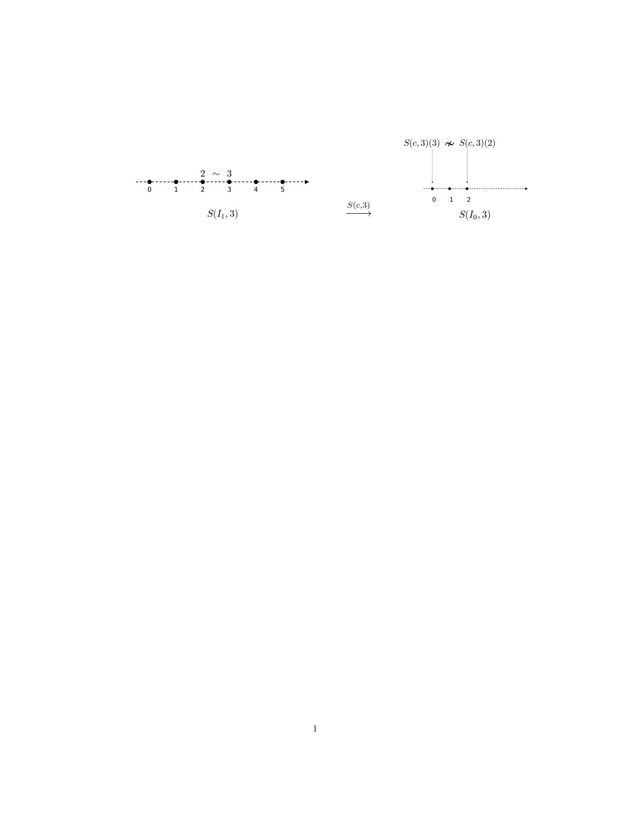 Figure 1
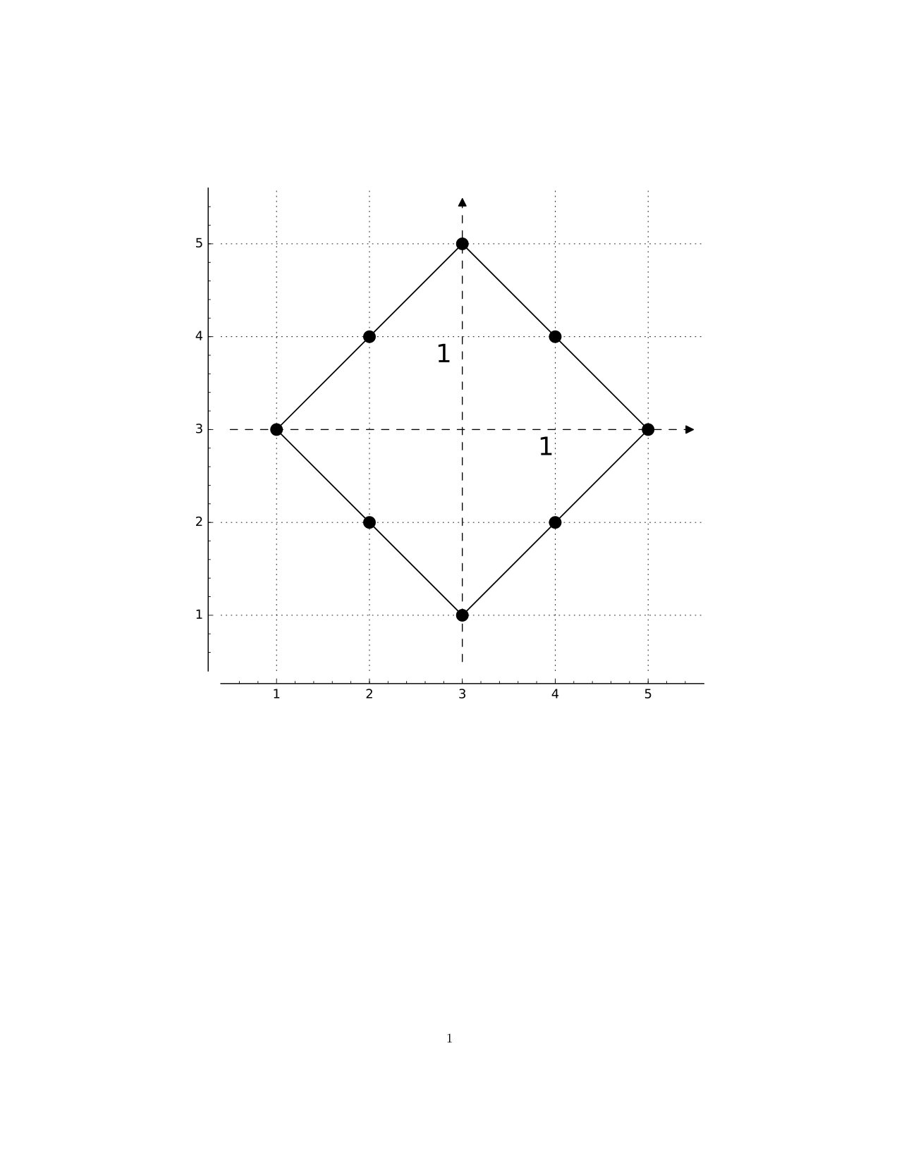 Figure 2
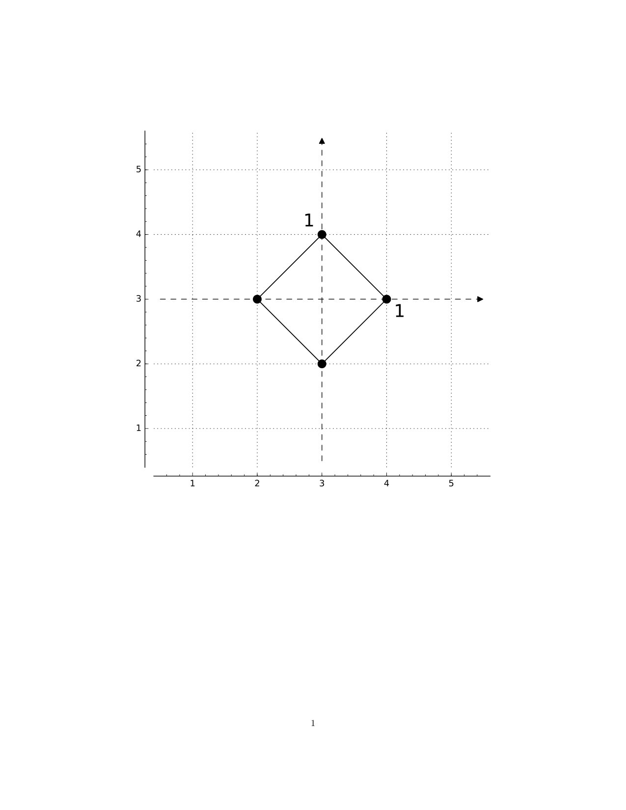 Figure 3
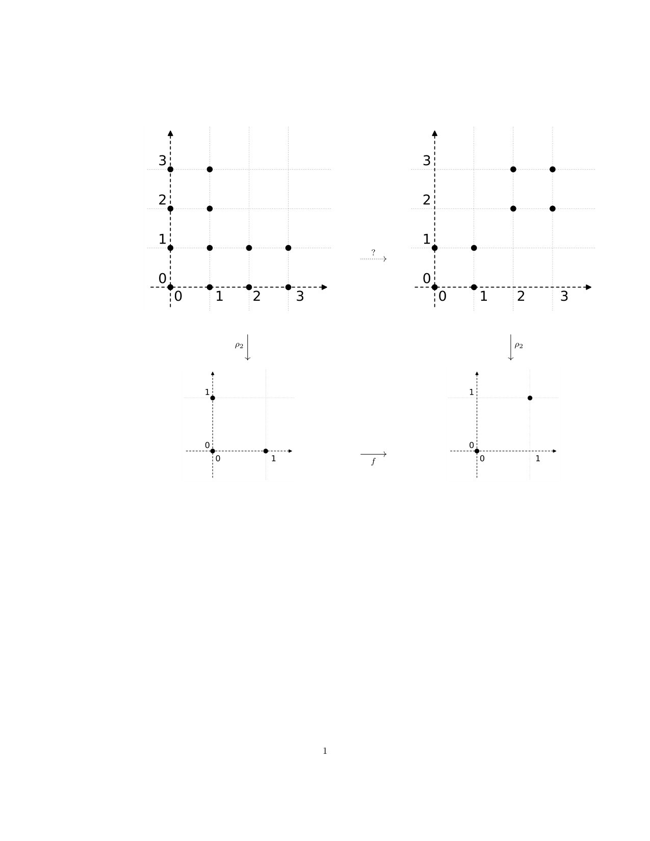 Figure 4
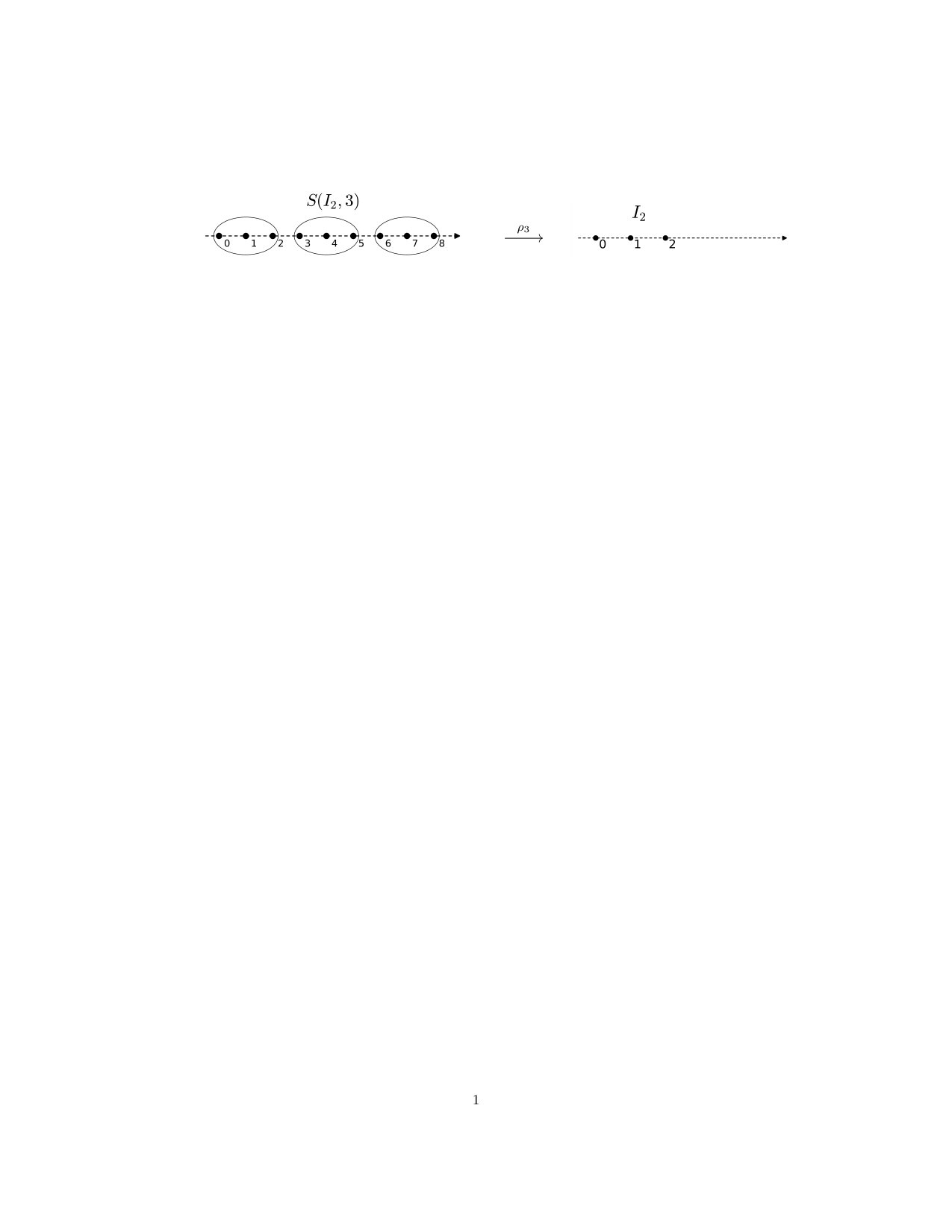 Figure 5
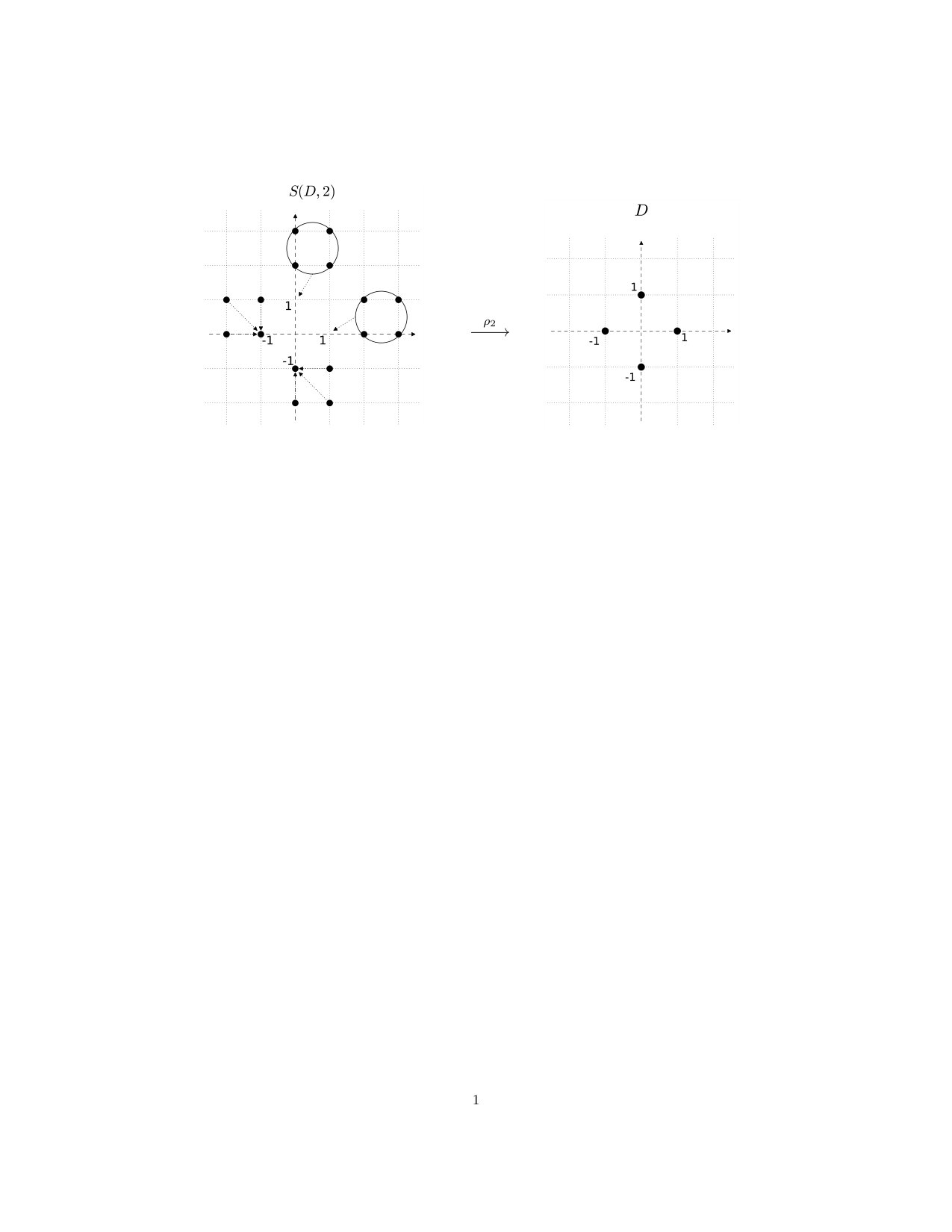 Figure 6
 Figure 7
 Figure 3
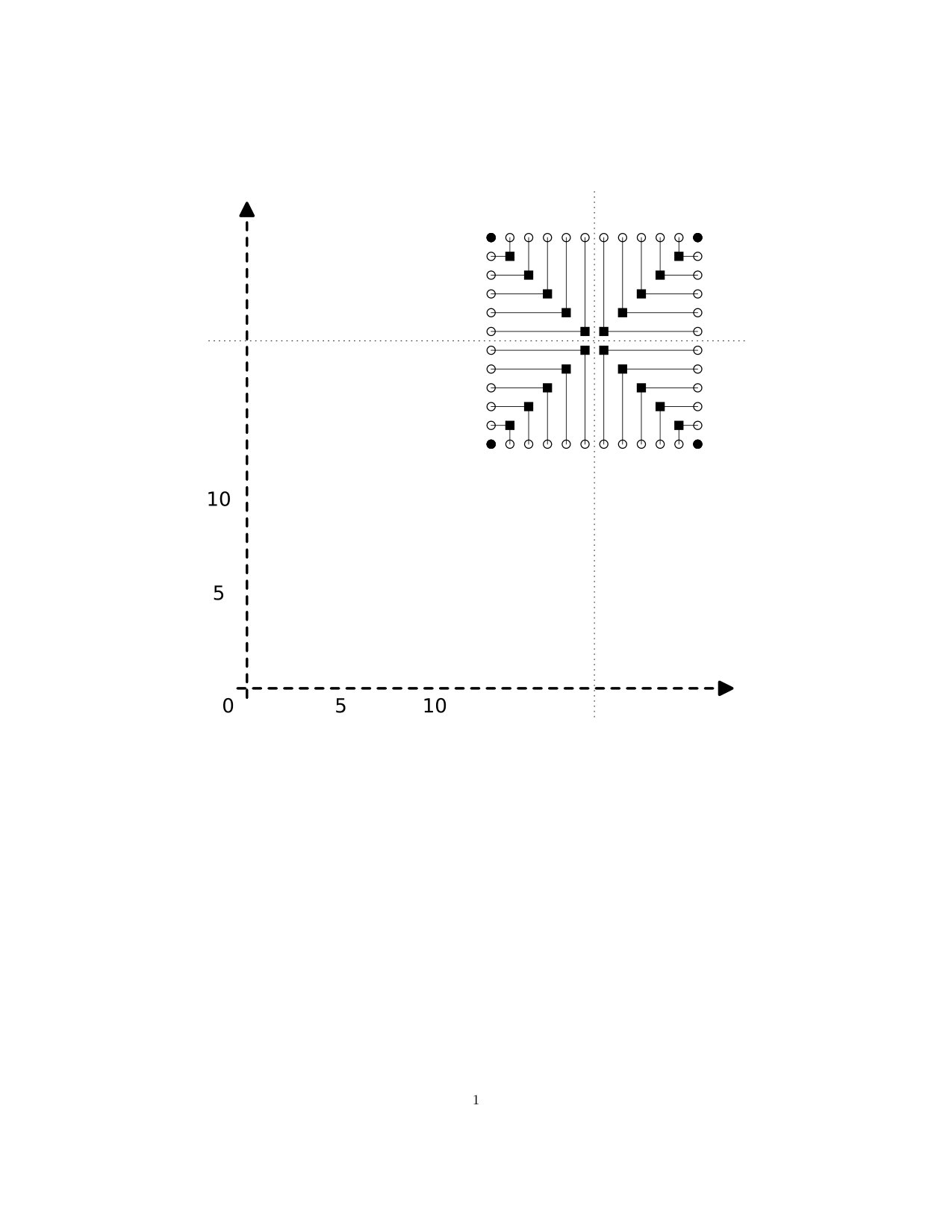 Figure 4
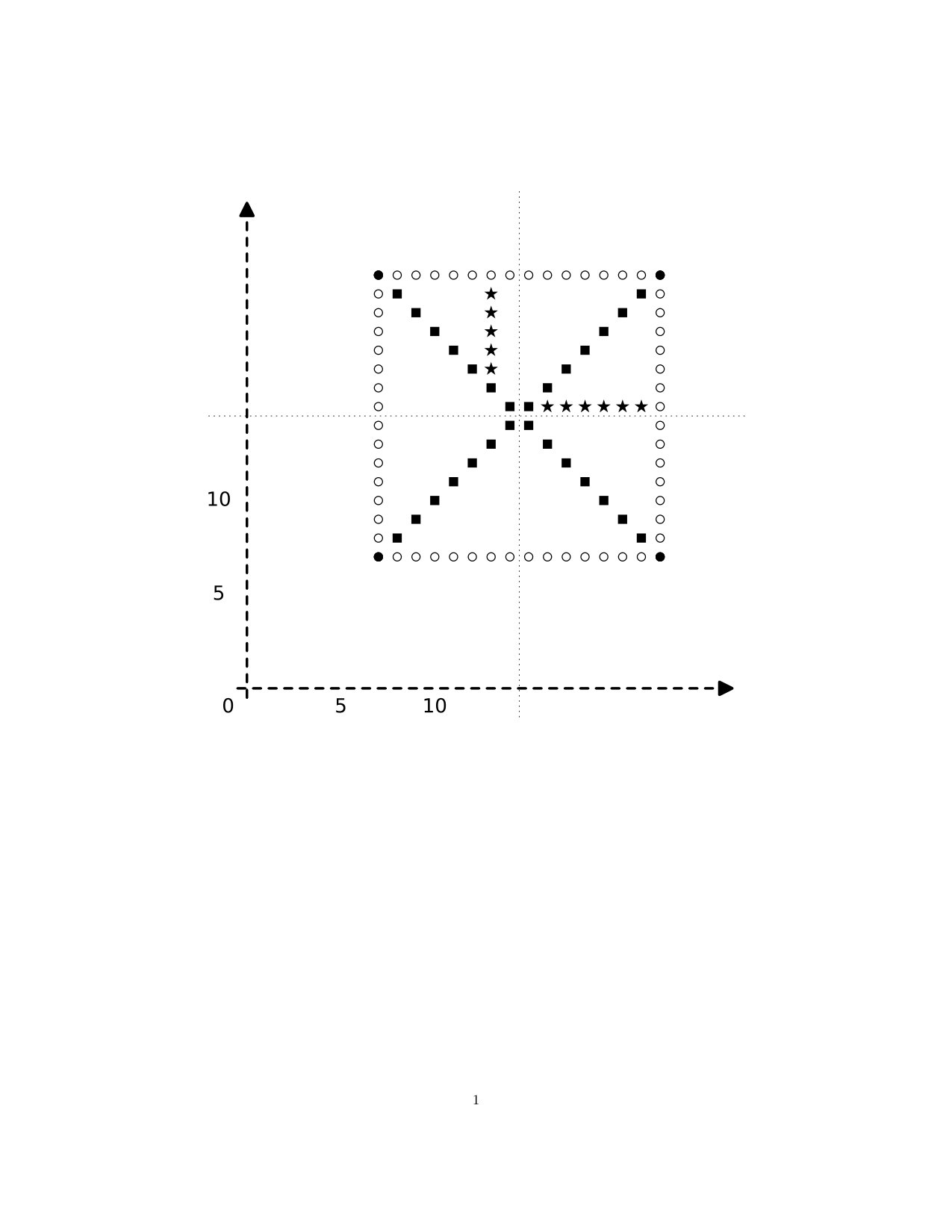 Figure 5
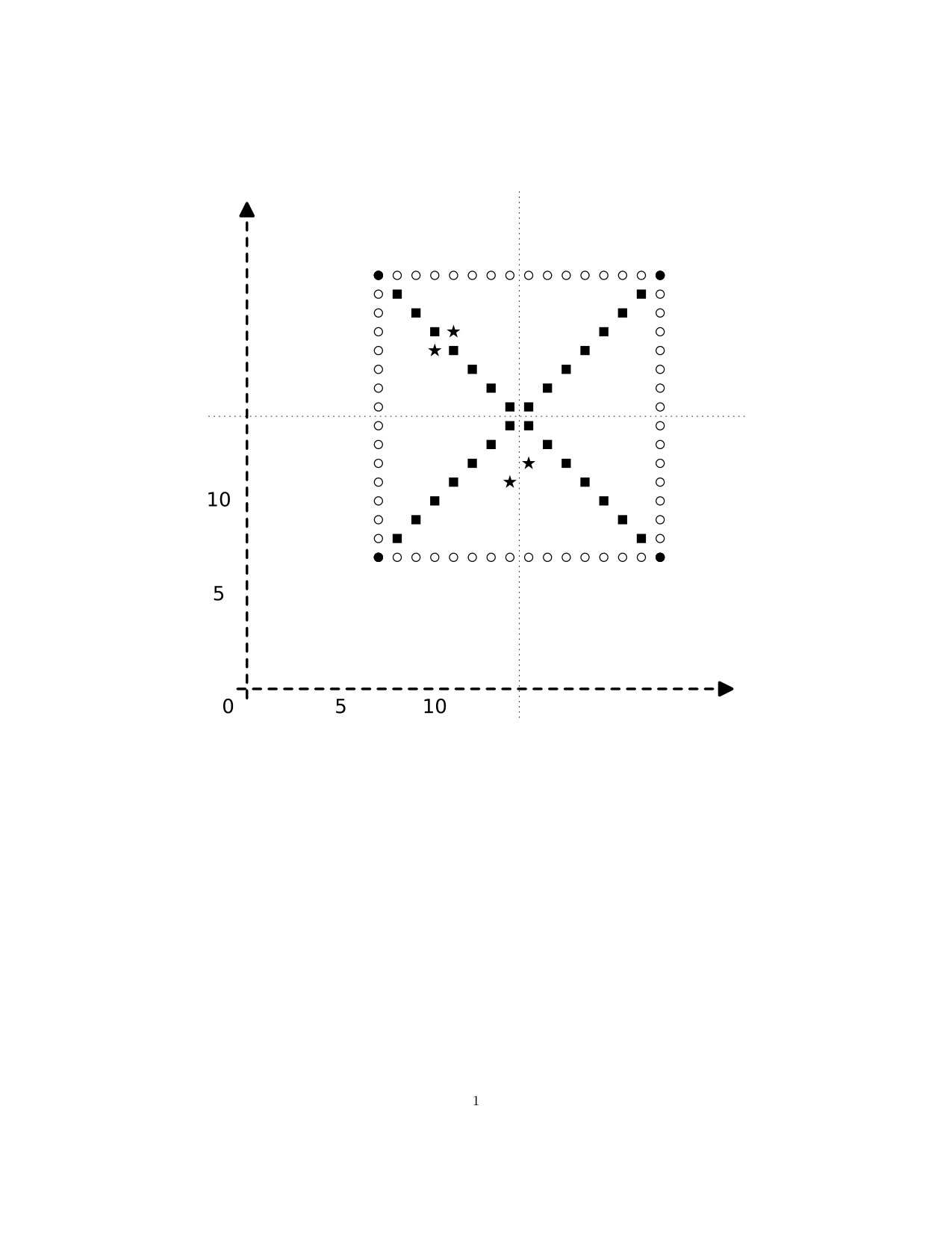 Figure 6
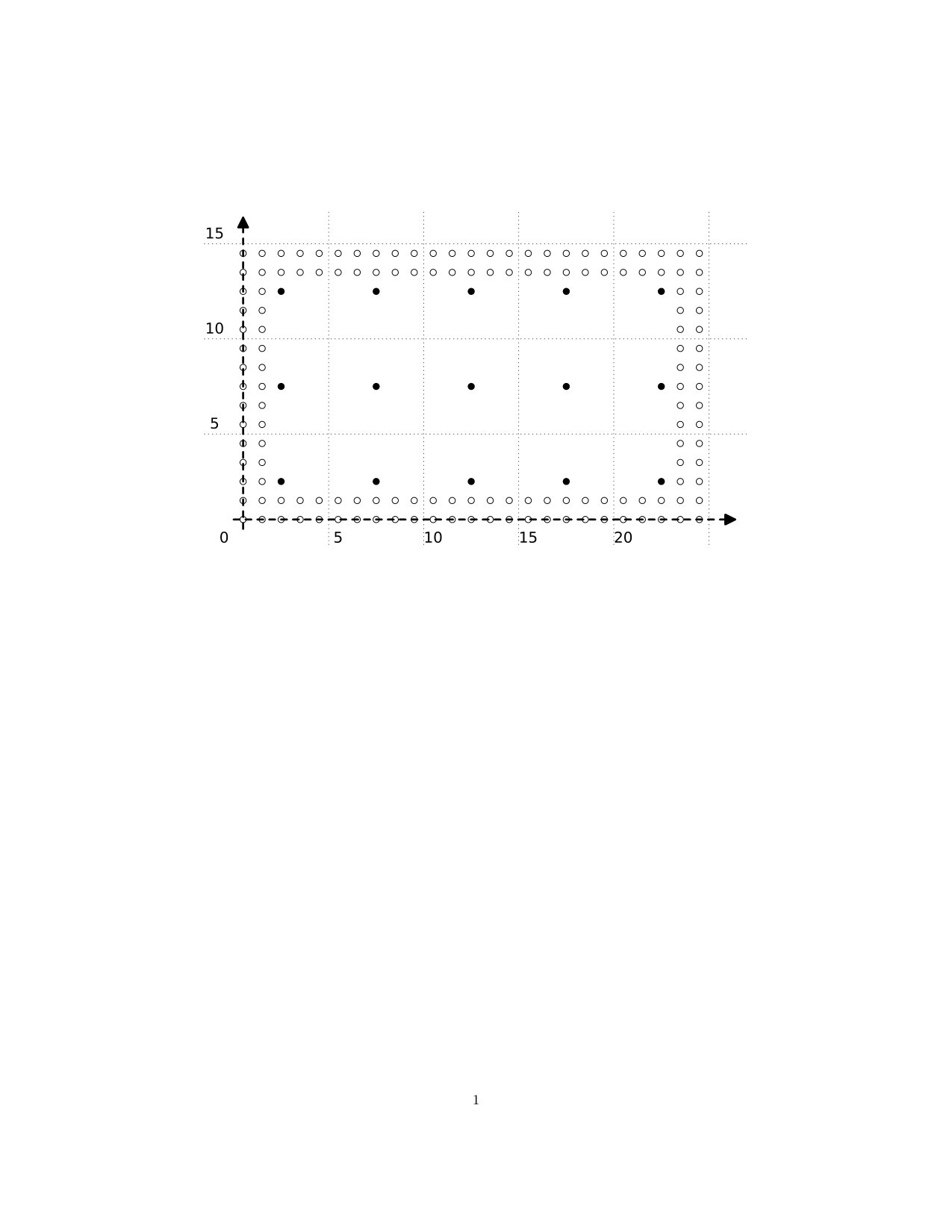 Figure 1
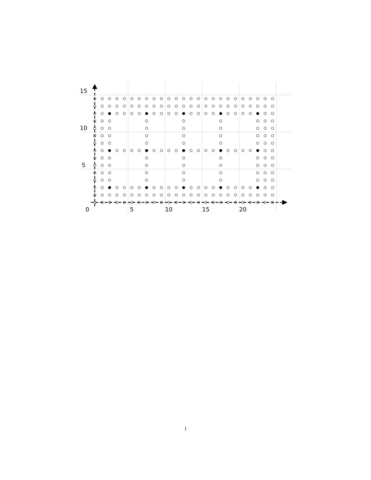 Figure 2
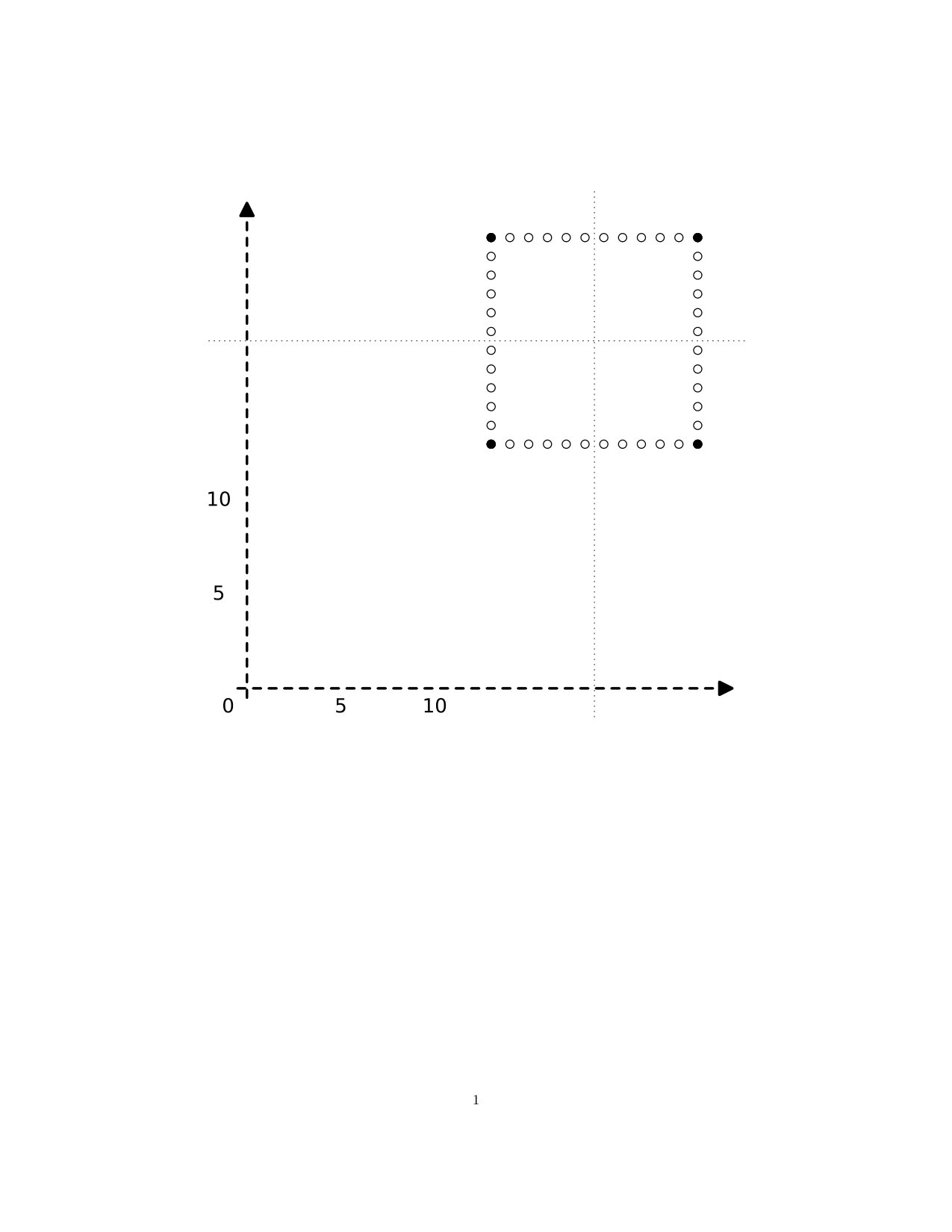 Figure 3
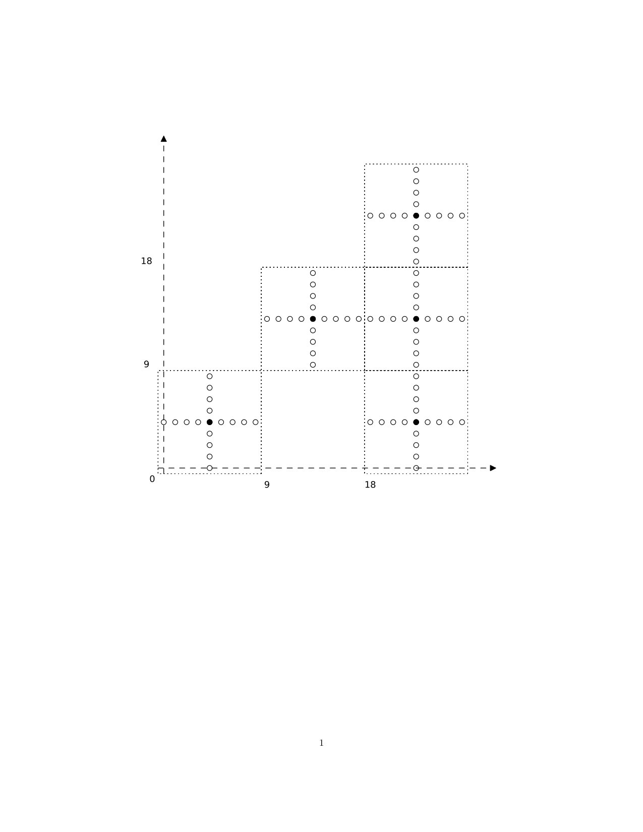 Figure 1
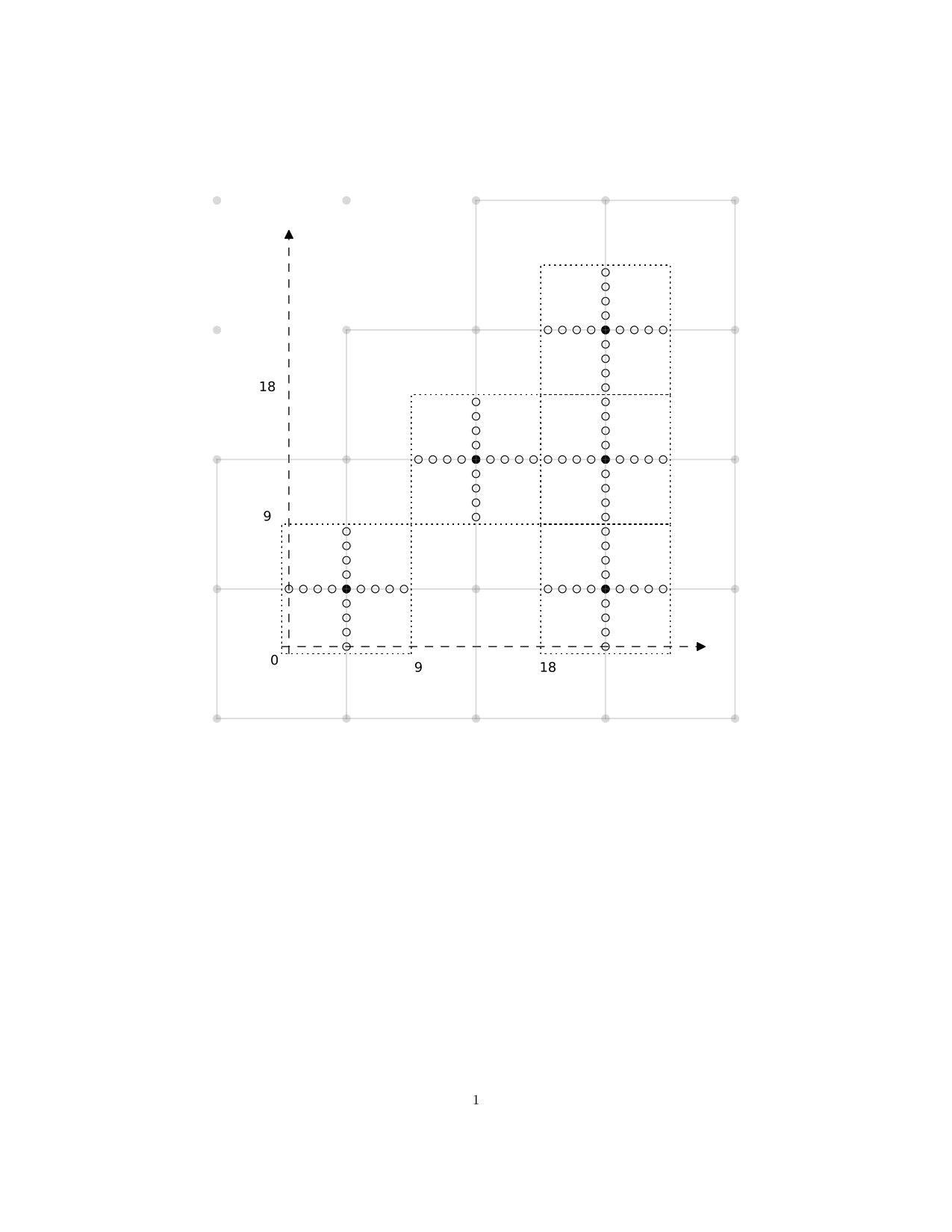 Figure 2
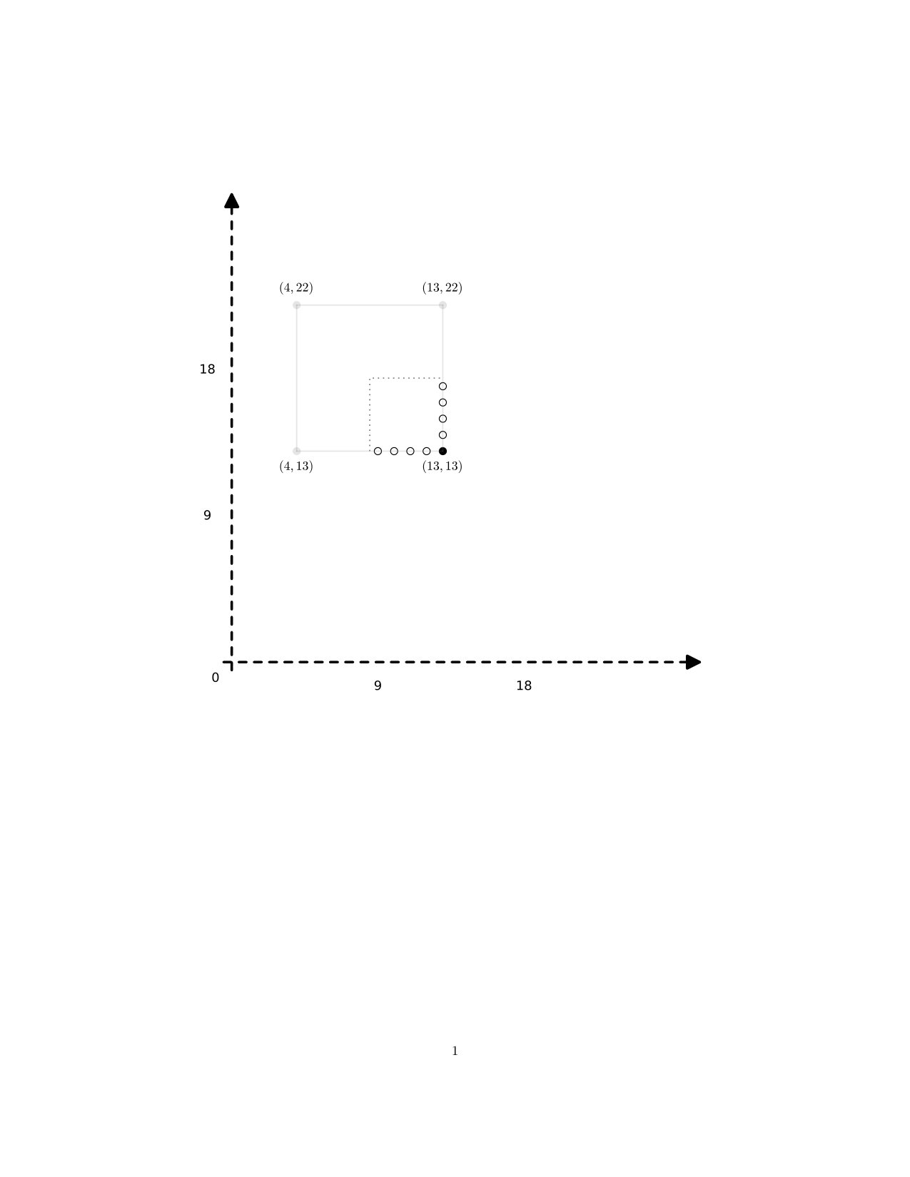 Figure 3
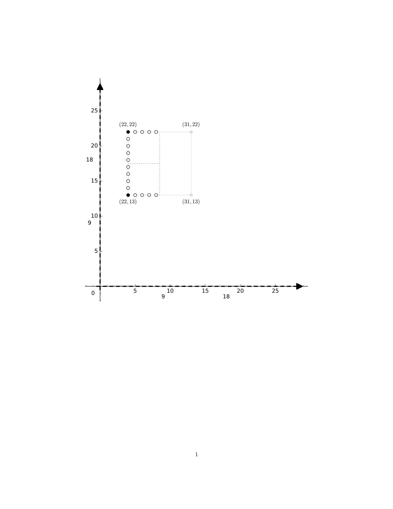 Figure 4
Peer Reviews
No public reviews on file for this paper yet. If you reviewed it on a platform where reviews are public (OpenReview, ICLR, NeurIPS, ICML), you can paste yours below so the community can read it here.
Videos
No videos yet. Explain this paper in a talk, walkthrough, or lecture? Add one.
Subdivision of Maps of Digital Images
Gregory Lupton
,
John Oprea
and
Nicholas A. Scoville
Department of Mathematics, Cleveland State University, Cleveland OH 44115 U.S.A.
Department of Mathematics and Computer Science, Ursinus College, Collegeville PA 19426 U.S.A.
Abstract.
With a view towards providing tools for analyzing and understanding digitized images, various notions from algebraic topology have been introduced into the setting of digital topology. In the ordinary topological setting, invariants such as the fundamental group are invariants of homotopy type. In the digital setting, however, the usual notion of homotopy leads to a very rigid invariance that does not correspond well with the topological notion of homotopy invariance. In this paper, we establish fundamental results about subdivision of maps of digital images with - or -dimensional domains. Our results lay the groundwork for showing that the digital fundamental group is an invariant of a much less rigid equivalence relation on digital images, that is more akin to the topological notion of homotopy invariance. Our results also lay the groundwork for defining other invariants of digital images in a way that makes them invariants of this less rigid equivalence.
Key words and phrases:
Digital Image, Digital Topology, Subdivision, Digital Fundamental Group, Lusternik-Schnirelmann category
2010 Mathematics Subject Classification:
(Primary) 54A99 55M30 55P05 55P99; (Secondary) 54A40 68R99 68T45 68U10
This work was partially supported by grants from the Simons Foundation: (#209575 to Gregory Lupton and #244393 to John Oprea).
1. Introduction
In digital topology, the basic object of interest is a digital image: a finite set of integer lattice points in an ambient Euclidean space with a suitable adjacency relation between points. This is an abstraction of an actual digital image which consists of pixels (in the plane, or higher dimensional analogues of such).
There is an extensive literature with many results that use ideas from topology in this setting (e.g. [8, 2, 5]). In many instances, however, notions from topology have been translated directly into the digital setting in a way that results in digital versions of topological notions that are very rigid and hence have limited applicability. In contrast to this existing literature, in [7] we have started to build a more general “digital homotopy theory” that brings the full strength of homotopy theory to the digital setting. In our approach, we aim to use less rigid constructions, with a view towards broad applicability and greater depth of development. A key ingredient in such an approach is subdivision. However, the behaviour of maps with respect to subdivision is not well-understood. In this paper, we establish fundamental results about subdivision of maps of digital images with -dimensional (1D) and -dimensional (2D) domains. The utility of our results is indicated in [6], in which we define a digital fundamental group and show that it is an invariant of subdivision-homotopy equivalence, which is a concept of “sameness” for spaces that is much less rigid than the notion of homotopy equivalence that is commonly used in digital topology. Our results of [7, 6], both in the basic constructions and in the developments, emphasize subdivision as a basic feature, whereas in those of [2] and many other articles in the digital topology literature, subdivision plays a background role at most. Our results here on subdivision of maps also allow us to define invariants of 2D digital images such as Lusternik-Schnirelmann category in a way that is much less rigid than previously done (e.g. as in [1]). In general, our results work towards establishing “subdivision versions” of the usual invariants. Our motivating point of view is that one should incorporate subdivision at a basic level, rather than directly translate a definition or construction from the topological to the digital setting. Incorporating subdivision results in digital invariants whose behaviour more closely follows that of their topological counterparts, when compared to the commonly used digital invariants that do not incorporate subdivision. To do this generally, however, requires a fuller understanding of the behaviour of maps with respect to subdivision—maps with domains of arbitrary dimension.
The paper is organized as follows. In Section 2 we review standard definitions and terminology, and set our conventions (especially with regard to adjacency). In Section 3 , we give a thorough discussion of subdivision of digital images and maps of digital images. We show how subdivision may be broken down into a succession of partial subdivisions (Corollary 3.8). Several figures are included that serve to indicate the basic ideas and concerns. The main question, illustrated through examples, is how—or even whether—a map of digital images induces one on subdivisions. In Section 4, we resolve this question for maps of digital images whose domain is an interval, namely paths and loops in a digital image (of any dimension). In Section 5 we do likewise for maps whose domain is a 2D digital image. In each case, we construct a canonical map of subdivisions from a given map of digital images. The main results are Theorem 4.1 and Theorem 5.5. A brief indication of the way in which our results here may be applied is given in Section 6. But applications of and developments from these results appear elsewhere. There, we also indicate how our results here on subdivision of maps lay the groundwork for future developments.
2. Basic Notions: Adjacency, Continuity, Products
In this paper, a digital image (of dimension ) means a finite subset of the integral lattice in some -dimensional Euclidean space, together with a particular adjacency relation inherited from that of . Namely, two points and are adjacent if their coordinates satisfy for each .
Remark 2.1*.*
In the literature, it is common to allow for various choices of adjacency. For example, a planar digital image is a subset of with either “-adjacency” or “-adjacency” (see, e.g. Section 2 of [2]). However, in this paper, we always assume (a subset of) has the highest degree of adjacency possible (-adjacency in , -adjacency in , etc.). In fact, there is a philosophical reason for our fixed choice of adjacency relation: It is effectively forced on us by the considerations of Definition 2.3 and Example 2.5 below.
If , we write to denote that and are adjacent in . For digital images and , a function is continuous if whenever . By a map of digital images, we mean a continuous function. Occasionally, we may encounter a non-continuous function of digital images. But, mostly, we deal with maps—continuous functions—of digital images. The composition of maps and gives a (continuous) map , as is easily checked from the definitions.
An isomorphism of digital images is a continuous bijection that admits a continuous inverse , so that we have and , and is also bijective. If is an isomorphism of digital images, then we say that and are isomorphic digital images, and write .
Example 2.2**.**
We use the notation for the digital interval of length , namely consists of the integers from [math] to in , and consecutive integers are adjacent. Thus, we have , , and so-on. Occasionally, we may use to denote the singleton point . As an example in , consider what we call the Diamond, , which may be viewed as a digital circle. Note that pairs of vertices all of whose coordinates differ by , such as and here, are adjacent according to our definition. Otherwise, would be disconnected.
In Figure 1 we have included the axes (dashed) and also indicated adjacencies (solid) in the style of a graph. Note, though, that we have no choice as to which points are adjacent: this is determined by position, or coordinates, and we do not choose to add or remove edges here. As an example in , we have (the vertices of an octahedron, with adjacencies corresponding to the edges of the octahedron). This may be viewed as a digital -sphere, and the pattern emerging here may be continued to a digital -sphere in with vertices. The map given by , , and is continuous, but the function given by , is not: we cannot “stretch” an interval to a longer one. Likewise, suppose we enlarge to the bigger digital circle (see Figure 1). Then the only maps will be “homotopically trivial:” we cannot “wrap” a smaller circle around a larger one.
The last comment of the preceding example points to the main motivation for the results of this paper. Whereas homotopy is not the main focus of this paper (the notion is reviewed here in Section 6), our results here are motivated by wanting to relax the notion of homotopy equivalence commonly used in digital topology. We can give the basic idea informally, as follows. Because we cannot “wrap” a smaller circle around a larger one, digital circles of different sizes are not homotopy equivalent, in the sense commonly used in digital topology. But from a (topological) homotopy point of view, it seems reasonable to view and as above—more generally, digital circles of different sizes—as being equivalent. In [7, 6], we develop a notion of subdivision-homotopy equivalence of digital images, which is a notion of “sameness” of digital images that combines subdivision with homotopy equivalence, and which is a less rigid notion of “sameness” than digital homotopy equivalence. Indeed, it turns out that and are subdivision-homotopy equivalent, but not homotopy equivalent. The comments made here about and are discussed in detail in Exercise 3.22 of [6].
Definition 2.3** (digital products).**
The product of digital images and is the Cartesian product of sets with the adjacency relation when and .
In fact, this is tantamount to our assumption that , and any digital image in it, has the highest degree of adjacency possible, with the isomorphisms for . Note that some authors in the literature use a different adjacency relation on the product: the graph product, whereby is adjacent to if and , or and . The notion we use is sometimes called the strong product, in a graph theory setting. Our definition of (adjacency on) the product means that it is the categorical product, in the category of (finite) digital images and digitally continuous maps. This point is explained in the following statement.
Lemma 2.4**.**
For digital images and , the projections onto either factor and are continuous. Suppose given maps of digital images and . Then there is a unique map, which we write that satisfies and .
Proof.
The first assertion follows immediately from the definitions. The map is defined as (f,g)(a)=\big{(}f(a),g(a)\big{)}. It is immediate from the definitions that this map is continuous. This is evidently the unique map with the suitable coordinate functions. ∎
Example 2.5**.**
For a digital image, the diagonal map
[TABLE]
is defined as for each . Suppose we have , with . Since , we need if the diagonal is to be continuous, which of course we do have with our conventions.
Because of the rectangular nature of the digital setting, it is often convenient to consider the product of maps, as follows.
Definition 2.6**.**
Given functions of digital images for , we define the product function
[TABLE]
as (f_{1}\times\cdots\times f_{n})(x_{1},\ldots,x_{n})=\big{(}f_{1}(x_{1}),\ldots,f_{n}(x_{n})\big{)}.
Lemma 2.7**.**
Given continuous maps of digital images for , their product is a (continuous) map.
Proof.
This follows directly from the definitions. ∎
We will make use of the product of maps towards the end of the following section and in the sequel. This gives another reason for why we want the product of digital images to be defined as in Definition 2.3.
3. Subdivision
The notion of subdivision of a digital image plays a fundamental role in our development of ideas in the digital setting, and is a main focus of this paper.
Definition 3.1**.**
Suppose that is an -dimensional digital image. For each , we have the -subdivision of , which is an auxiliary (to ) -dimensional digital image denoted by , together with a canonical map or standard projection
[TABLE]
that is continuous in our digital sense. For a real number , denote by the greatest integer less-than-or-equal-to (the integer floor of ). First, make the -lattice in , namely, those points with coordinates each of which is for some integer , and then set
[TABLE]
Then set
[TABLE]
The map is given by \rho_{k}\big{(}(y_{1},\ldots,y_{n})\big{)}=(\lfloor y_{1}/k\rfloor,\ldots,\lfloor y_{n}/k\rfloor), and one checks that this map is continuous.
For an individual point, we write for the points that satisfy . If is a point in an -dimensional digital image, then we may describe this set in general as
[TABLE]
That is, for each , is an -dimensional cubical lattice in with each side of the cubical lattice containing points. Notice that the result of subdivision therefore depends on the ambient space of the digital image.
Occasionally, it may be convenient to extend Definition 3.1 to include , in which case we use the notational convention that , and is just the identity map of .
Example 3.2**.**
Generally, subdivision of an interval gives a longer interval: We have . Suppose that we have . Then we have , and is given by , , and . In Figure 2, we indicate the way in which, for the same interval , the projection aggregates points in the subdivided interval to map them back to the original.
We also note here that
As a two-dimensional example, suppose that we have . Then , and we have given by , and . Finally, in Figure 3, we show the points of , with the diamond as in Figure 1 above, and indicate the way in which the points of are aggregated by the projection .
Subdivision behaves well with respect to products. For any digital images and and any we have an isomorphism of digital images
[TABLE]
and, furthermore, the standard projection may be identified with the product of the standard projections on and , thus:
[TABLE]
Note also that we may iterate subdivision. It is straightforward to check that, for any , we have an isomorphism of digital images S\big{(}S(X,k),l\big{)}\cong S(X,kl).
Example 3.3**.**
We mentioned above that, for , we have . For the origin , we have , an -cube in , and we may identify the projection as a product of projections
[TABLE]
More generally, for any , we have
[TABLE]
If , then we have
[TABLE]
These descriptions make plain that we may identify the projection with the product of projections
[TABLE]
By an inclusion of digital images (of the same dimension) we mean that is a subset of (the coordinates of a point of remain the same under inclusion into ). It is easy to see that, given an inclusion of digital images , we have an obvious corresponding continuous inclusion of subdivisions such that the diagram
[TABLE]
commutes. We say that the map covers the map . Indeed, we may give an explicit formula as follows. For each point , write . Also, write , with , for a typical point in the cubical lattice . Then the points of may be written as
[TABLE]
with for all . Here, the scalar multiple and the sum denote coordinate-wise (vector) scalar multiplication and addition in . Then may be written as
[TABLE]
where . It is easy to confirm that this gives a (continuous) map.
For a more general map , however, it is not so clear how we should construct a map of subdivisions that covers the map, in the sense of a filler—a map that occupies the place of the dotted arrow—for the following (commutative) diagram:
[TABLE]
In fact, it is not even obvious that such a map of subdivisions always exists, in general. In this paper we show that such a map does exist for arbitrary maps of digital images with 1D and 2D domains. However, as the next several examples illustrate, the formulation of (2) will not provide such a map in general.
Example 3.4**.**
Consider the constant map of 1D digital images , given by . If we use the formulation of (2) above to define a function
[TABLE]
as S(c,k)\big{(}k\,a+t\big{)}=k\,c(a)+t, then we have but . Then but unless : the function is not continuous for . See Figure 4 for an illustration of this situation.
In this example, defining as a constant map, , for instance, gives a continuous map that covers . But the point here is, that it is not obvious how to adapt a covering map of subdivisions depending on the given map.
The issue is not confined to functions that coalesce points together, either. Here are two examples of injective maps for which , defined as in (2) above, fails to be continuous.
Example 3.5**.**
(a) Consider the map given by and . The function defined by the formulation of (2) above gives
[TABLE]
Since , this function is not continuous for any . See Figure 5, in which we have indicated the way in which the projections aggregate points.
(b) (Similar to an observation illustrated in [3, Fig.1].) Consider the map with , , and given by
[TABLE]
The function defined by the formulation of (2) above gives
[TABLE]
on the four points of S\big{(}(0,0),2\big{)}. Likewise for the four points in S\big{(}(1,0),2\big{)}, would give
[TABLE]
But this would result in adjacent points being mapped to non-adjacent points , for example. The situation is summarized in Figure 6, in which we want a filler that makes the diagram commute. Notice one feature of this example, in particular. Although we have , it is not possible for a covering map of to restrict to the identity S\big{(}(0,0),k\big{)}\to S\big{(}(0,0),k\big{)}. For , for instance, we see in Figure 6 that and , but any covering map of must map both and to points of S\big{(}(1,1),2\big{)} in , none of which are adjacent to . That is, the possibilities for a covering map are constrained by how surrounding points are mapped by , and not just by how the points themselves are mapped. In this example, it is not so clear how one should associate a continuous map to the original , as part of a methodical scheme for doing so.
In the next two Sections, we will give methodical constructions that, in particular, provide covering maps of subdivisions in the examples above. A more general question, special cases of which are also resolved in the following sections, is to ask how—or whether—a map of digital images of different dimensions might induce a covering map of subdivisions.
We close this section on subdivision with some constructions that we use in the following section and in the sequel. The projection may be factored—written as a composition—in various ways. For example, if , then we may write
[TABLE]
A different sort of “partial projection” that may also be used to factor is as follows.
Definition 3.6**.**
For any and any , recall that the subdivision may be described as . Then, for , define a function
[TABLE]
as
[TABLE]
Next, for any , with the identifications from Example 3.3 of
[TABLE]
and
[TABLE]
define as the product of functions
[TABLE]
Finally, for any digital image , define
[TABLE]
by viewing each subdivision as a (disjoint) union
[TABLE]
and assembling a global on from the individual as just defined.
Proposition 3.7**.**
For , the partial projection is continuous.
Proof.
For , the map of intervals is easily seen to be continuous. Then, for any , we have defined as the product of individually continuous functions, hence it is also continuous. It remains to confirm that the assemble together to give a globally continuous function on .
So suppose that we have and with and . Note, though, that we must have , since , , and is continuous. Write and . Then we have
[TABLE]
for with , each . Now for , it is necessary and sufficient that we have in , for each . Write and , with the satisfying and determined as in Definition 3.6. Then
[TABLE]
and we must show that, for each , we have
[TABLE]
Because we have , it follows that, for each , we have . For each , there are three possibilities. First, suppose that we have . Then entails that, in the th coordinates, we have
[TABLE]
Thus and the only possibility is that, in this coordinate, we have and . From Definition 3.6, then, we have and and hence , which satisfies (3). Second, suppose that we have . Then
[TABLE]
thus , and we have and . From Definition 3.6, then, we have and and in this case , which also satisfies (3). Finally, suppose that we have . Here, entails that we have
[TABLE]
so that and differ by at most . From Definition 3.6, if or if , then we have and so . The only other possibility is that we have in which case and so . Wherever and fall in , then, we have which satisfies and (3) is again satisfied. The result follows. ∎
Corollary 3.8**.**
Let be any digital image. For any , we may factor the projection as
[TABLE]
with the standard projection and the partial projection map from Definition 3.6.
Proof.
It is sufficient to check that the composition agrees with on , for each . But when restricted to , both and are constant maps. ∎
4. One-Dimensional Domains: Paths and Loops in
For a digital image and any , a path of length in is a continuous map . Unlike in the ordinary (topological) homotopy setting, where any path may be taken with the fixed domain , in the digital setting we must allow paths to have different domains. Recall from Example 3.2 that we obtain a longer interval when we subdivide an interval: .
In the following result, notice that the map of subdivisions that covers the given path is itself a path (of length ) in the subdivided digital image .
Theorem 4.1**.**
Suppose we are given , a path of length in any digital image . For any odd , there is a canonical choice of map of subdivisions
[TABLE]
that covers the given path, in the sense that the following diagram commutes:
[TABLE]
Our proof consists of an algorithmic construction of the covering map (or path) . We first establish some notation and vocabulary used in the proof. For the above diagram to commute, it is necessary and sufficient that the map be a “fibrewise” map, in the sense that it satisfies
[TABLE]
for each and . If is a typical point in the interval, write . Thus, is the point in the centre of the length subinterval and, in particular, we have , with the standard projection. Then the points of each may be described as
[TABLE]
To describe points of , we use notation similar to that used above in the discussion of covering an inclusion. For each point , write if . Then, write \overline{y}=\big{(}(2k+1)y_{1}+k,\ldots,(2k+1)y_{n}+k\big{)}\in S(y,2k+1), so that is the point in the centre of , which is a cubical lattice in . Namely, is the translate of by . Here, the scalar multiple means coordinate-wise (vector) scalar multiplication, and we will use coordinate-wise (vector) scalar multiplication and addition in freely in our notation. Note, in particular, that we have , with the standard projection. Then the points of each may be described as
[TABLE]
Proof of Theorem 4.1.
We define our covering map of subdivisions
[TABLE]
in such a way so that we have
[TABLE]
for each . That is, we will map the centre of the subinterval to the centre of the cubical lattice , for each . Now the key point to realize here is that, for any pair of adjacent points , the centres of and are joined by a (straight) segment of length , consisting of points—including the two centres themselves as endpoints of the segment. Of these points, of them, including , are contained in and of them, including , are contained in . To define , then, we simply “join the dots” between the centres of the cubical lattices, using the points of between the centres of the subintervals to map point-for-point to the segments joining the centres of the lattices in .
To define this map in symbols, which we do in formulas (12) and (13) (see also (14)) below, we write for the “displacement vector” in from to , for each . Since , each coordinate of is [math], , or . For each with , we may write
[TABLE]
for unique and with . Indeed, if falls in a subinterval of form
[TABLE]
for some with , then we have and is in the range . On the other hand, if falls in a subinterval of form
[TABLE]
for some with , then we have but here and is in the range .
Also, write for the vector each of whose coordinates is . Then, for each , the two centres and in that correspond to the adjacent points and in have coordinates that satisfy
[TABLE]
Thus, we may pass from to by successively adding the displacement vector to a total of times. This is the segment of points in joining the neighbouring centres alluded to above.
Our formula for , then is given as follows: For , with the above notation, we define on the parts of before the first centre and beyond the last centre as
[TABLE]
and on the part of that falls between (any) centres as
[TABLE]
We may also write (13) as follows, in a way that perhaps emphasizes the interpolation between centres. First, write the domain of definition of (13) as the disjoint union
[TABLE]
where we have , whence . Also, for each , if we write as for some with , then and so and from (8). Then, for each , (13) may also be written:
[TABLE]
First observe that this definition does indeed satisfy the “centre-to-centre” property (7). For if , Formula (12) gives . If , then (8) (or (9)) gives and , whence Formula (13) (or (14)) gives .
Next we confirm that, with this definition, the desired diagram commutes. For this, we confirm that has the fibrewise property of (4). Divide into a (disjoint) union of subintervals of the form
[TABLE]
with the first type of subinterval consisting of the points to the left of a centre and the second type consisting of the points to the right (including the centre itself). Note that we have
[TABLE]
for each (see (5) above).
For with , formula (10) and the expressions that follow it give and in the range . From formula (13) we have
[TABLE]
where the re-write in the second line follows from (11). Since we have and the displacement vector has coordinates from , it follows from (6) that we have
[TABLE]
for .
Similarly, for with , we have and (cf. (9) above). Then
[TABLE]
from (6), because the displacement vector has coordinates from . Hence, we also have
[TABLE]
for .
Finally, Formula (12) gives directly that and . These items combined with (16), (17), and (15) confirm that (4) is satisfied for each .
For continuity, since is a path in , we simply need to check that for each . To this end, write as a (disjoint) union of subintervals of the form
[TABLE]
On each of these subintervals separately, is easily seen to be continuous. In fact, is constant on the first and last. Using (8)–(10), we may write each of the remaining intervals as
[TABLE]
On , then, Formula (13) gives us
[TABLE]
with as we take successively from to . Now each displacement vector has coordinates taken from , and so when we add this term to a point in , as we are doing here in passing from to , we adjust each coordinate by at most to yield an adjacent point in .
The remaining issue, then, is whether these continuous segments match-up in a continuous way. For the first pair, namely and , we have , and so certainly gives a continuous map on the union of these two subintervals. For the remaining pairs of adjacent subintervals, we must check that and are adjacent, for . Using (18) and the displayed formula below it for reference, we have
[TABLE]
where we have used (11) to arrive at the middle line. Once again we use the fact that each has coordinates taken from to conclude that and are adjacent, and so does indeed assemble into a continuous function. ∎
Example 4.2**.**
Return to part (a) of Example 3.5 and consider the map given by and . Applying Theorem 4.1, we obtain a map
[TABLE]
that covers . It is given by for , and , .
Example 4.3**.**
Let be a constant path in . Suppose that we have for . For any odd , the map given by Theorem 4.1 that covers is simply the constant path for . For instance, we would cover the constant map in Example 3.4 with the constant map with for each .
We will refer to the cover of a path constructed in Theorem 4.1 as the standard cover of the path. Ideally, we would like to construct a functorial cover of maps of digital images regardless of the dimension of the domain, but we are not able to do so at present. We observe here, though, that the standard cover of a path does have some functorial-like properties, such as the following:
Lemma 4.4**.**
Let be any digital image. For any path , let denote the standard cover with respect to -fold subdivisions, so that makes the following diagram commute:
[TABLE]
- (a)
If denotes the constant path at a point , then we have , the constant path at , where .
- (b)
If and is the identity, then we have
[TABLE]
Proof.
Both parts follow from a careful reading of the definition of . ∎
Remark 4.5*.*
The conclusion of Theorem 4.1 holds also for even subdivisions. However the proof of this, whilst following essentially the same strategy as that of Theorem 4.1, involves an adaptation to the fact that we have no “middle points” in an even subdivision. To avoid giving another lengthy argument, much of which would be repetitive of the one just given, we settle instead for the weaker result below, which is sufficient for our purposes here.
Still, we briefly indicate the way in which the proof of Theorem 4.1 may be adapted. Recall that by an -clique in a digital image, we mean a set of points, each pair of which is adjacent. For even subdivisions of , each cubical lattice has a central -clique in place of the centre . For an interval, has a central -clique, or middle pair. To construct a covering map , we begin by mapping central -cliques to central -cliques (a choice is involved, which is determined by the “displacement vectors” used in the proof of Theorem 4.1), and then stringing these together using the remaining points of . If we imagine our central -cliques as “lights” at the centre of each cubical lattice, then the covering paths here are akin to a string of (higher-dimensional) fairy lights, with each light joined by a straight segment of wire.
In the following, the conclusion for the case in which is odd is actually weaker than that of Theorem 4.1. We include it here so as to have a statement of the fact that a covering map exists independently of the parity of .
Corollary 4.6**.**
Suppose we are given , a path of length in any digital image . For any , there is a map of subdivisions
[TABLE]
that covers the given path, in the sense that the following diagram commutes:
[TABLE]
Proof.
Suppose that is even. Pre-compose with the “partial projection” of Definition 3.6. Then, as in Corollary 3.8, we have and Theorem 4.1 provides a filler for the diagram
[TABLE]
But then provides the desired covering of .
Similarly, if is odd, then use . ∎
We end this section with a companion result about subdivision of loops in a digital image.
Definition 4.7**.**
A loop of length in a digital image is a path that satisfies .
Corollary 4.8**.**
Suppose we are given , a loop of length in any digital image . Suppose that we have . For any , there is a map of subdivisions
[TABLE]
with , that covers the given loop, in the sense that the following diagram commutes:
[TABLE]
Furthermore, is a loop, of length in , and we may take to be a loop based at any point of .
Proof.
A review of the definitions of the covering paths in Theorem 4.1 and reveals that the standard cover of the loop is a loop based at if is odd, or at , where , if is even. (Note that is odd, whether is odd or even.) In both results, the covering paths started and ended with a constant portion, of “duration” equal to one-half the width of the appropriate cubical lattice. For any , rather than keep these ends constant, we treat them as “loose ends,” which then may be used so as to complete the loop at a different basepoint of if desired. ∎
5. Two-Dimensional Domains: Surfaces in
We begin with a particular version of our main result. We consider the case in which the domain is a rectangle . In this case, we can give a rather clean and direct argument that generalizes the results of the previous section in a very satisfactory way. Also, this case leads to a useful corollary about covers of homotopies (Corollary 6.2), which we use in [6]. In the following proof, we rely heavily on the notation established for Theorem 4.1.
Theorem 5.1**.**
Suppose we are given a map with any digital image. For any , there is a canonical choice of map that makes the following diagram commute:
[TABLE]
Furthermore, if we define and , then , the standard cover as in Theorem 4.1 of the path . Likewise along the other three edges of the rectangle .
Proof.
For each with , define , and for each with , define , as
[TABLE]
So the are the horizontal coordinate curves of , and the are the vertical. Then as in Theorem 4.1, each of these paths has a standard cover
[TABLE]
and
[TABLE]
We will define in such a way as to have these be amongst the horizontal and vertical coordinate curves of , respectively.
Recall from our generalities on subdivision in Section 3 that we have an isomorphism of digital images . For individual points , we may specialize this identification to an isomorphism S\big{(}(i,j),2k+1\big{)}\cong S(i,2k+1)\times S(j,2k+1). We use these identifications repeatedly in what follows.
Recall also from Theorem 4.1 that, for , we write the centre of the subinterval as . Then each sub-lattice S\big{(}(i,j),2k+1\big{)}\subseteq S(I_{M}\times I_{N},2k+1) has the point
[TABLE]
at its centre. We refer to these points as centres of the sub-divided digital image . Furthermore, for a point , we write for the centre of .
We may begin by defining on these centres as
[TABLE]
for each . We will extend this definition of over the whole of in several steps.
5.1.1. Step 1: Outside the centres
For or , or or define
[TABLE]
The situation is illustrated in Figure 7. Dots represent the points on which has been defined at this point. Solid dots represent centres, on which we have defined as in (19). Open dots are those points on which we have defined at this step. We have also included some gridlines (dotted) in the figure. These gridlines do not pass through points (they are not gridlines of the integer lattice). Rather, they pass between points, and serve to aggregate points into squares in , of the form
[TABLE]
for . Each of these squares contains one center, namely \overline{(i,j)}\in S\big{(}(i,j),2k+1\big{)}. All points in one of these squares are mapped to one point of by the standard projection; we have \rho_{2k+1}\big{(}S\big{(}(i,j),2k+1\big{)}\big{)}=(i,j)\in I_{M}\times I_{N}.
Notice that where definitions from this step overlap with each other, namely in each of the four corner regions, the definitions agree. For example, if , we have and . Now, for , Theorem 4.1 gives , and similarly we have for . The other four corner regions behave similarly.
We will check continuity after the next step.
5.1.2. Step 2: Coordinate curves through the centres
Next we extend the definition of to the horizontals and verticals through each centre of . On these, we define for each and ,
[TABLE]
The situation is illustrated in Figure 8. Again, dots represent the points on which has now been defined. Solid dots represent centres; open dots represent points on which the definition of has been extended in Steps 1 and 2.
We check is well-defined. In any horizontal row or vertical column that includes centres, this Step 2 includes a definition of at those centres. Notice that the way in which we defined the standard cover of a path in Theorem 4.1 extended the “centre-to-centre” definition of (7), so the value assigned to on any centre at this step is consistent with the value assigned by (19). The only other overlap in definition is at the top or bottom of a vertical, or the left and right ends of a horizontal. For example, if , we have from this step, and from Step 1. Now , since , so we have . But , and the definitions agree. The other overlaps around the edges are seen to agree similarly; is well-defined thus far.
Now we check continuity, so far as we have defined . To this end, suppose we have adjacent points and in that part of on which we have defined . If both points are in one of the horizontal bands or , or if both points are in one of the horizontal rows through centres for some with , then adjacency of and in follows immediately from the continuity of the standard covers . This is because, on these horizontal regions, we have defined , for a suitable depending on . Hence, for , we have in , whence and therefore . For both points in one the vertical bands or , or both points in one of the vertical columns through centres for some , adjacency of and in follows immediately from the continuity of the standard covers , in a similar way.
It remains to consider the cases in which one point lies in a horizontal row or band, the other point lies in a vertical row or band, and they are situated “across a corner from each other” so that both do not lie in a horizontal or a vertical. This entails that one point is on a horizontal and one on a vertical, each adjacent, but not equal, to a centre (see Figure 8). For example, consider a pair and . Here, we have
[TABLE]
and
[TABLE]
The difference between these two, using vector arithmetic in , is
[TABLE]
Since is continuous, and in , each coordinate of this difference is in , and it follows that we have
[TABLE]
Similarly, consider the pair of points (towards the lower-right corner in Figure 8). Now , so we have (cf. formula (14) from Theorem 4.1)
[TABLE]
and, since we have (refer again to (14))
[TABLE]
Using vector arithmetic in , we may write and . The difference between and , then, is
[TABLE]
Now , and hence from the continuity of . It follows that each coordinate of , and hence each coordinate of , belongs to . That is, we have
[TABLE]
Other cases are checked similarly; we leave the details as an exercise. It follows that is continuous, so far as we have defined it.
5.1.3. Step 3: Extension over squares whose corners are centres
The last step requires some ideas beyond those of Theorem 4.1. But, first, note that we may extend over the interior of any square in whose corners are centres independently of any other such square. This is because any two points of that are adjacent must be in one such square (including its edges) or, if not, then both must be in the region of from Part 2, where we have already confirmed continuity. So it is sufficient to show that we may extend over a typical such square
[TABLE]
with corners
[TABLE]
for some . Such a square is illustrated in Figure 9. As in the two previous figures, dots indicate points on which we have already defined . Notice we have preserved portions of the gridlines discussed when we described the features of Figure 7 above. These gridlines now divide each square into four quadrants. Each quadrant contains a centre of (at its corner) and all points in one quadrant are mapped to one point of the -clique by the standard projection. It follows that, if we are to cover , the image under of all points in one of these quadrants must lie in some for a single point . For example, The lower-left quadrant of consists of the points and we require the extended to satisfy
[TABLE]
In the statement of Lemma 5.2 below, this “quadrant-wise” behaviour of an extension to a cover is addressed explicitly. Furthermore, as we progress with the proof of Lemma 5.2, we will depend heavily on having the square divided into quadrants in this way.
In the previous steps, we have already defined on the edges and corners of this square.
We will apply Lemma 5.2 below to extend over the interior of this square. To do so, use the given to determine a unit -cube as follows. On each point of write coordinate-wise as
[TABLE]
and so-on for the other points. Then, for each coordinate , set
[TABLE]
and let denote the unit -cube
[TABLE]
Then write
[TABLE]
so that maps each orthant of to the corresponding corner of . If, as in Lemma 5.2, we write
[TABLE]
for the boundary of the square , then from Steps 1 and 2 we have
[TABLE]
with each corner of mapped by to some corner of , and each edge of mapped to the corresponding edges or diagonals of . Notice this “corner-to-corner” assertion follows from our choice of the coordinates for the distinguished “minimal” corner of : Because is the minimum of , and because is continuous, it follows that we have
[TABLE]
for each point of the -clique . Notice also that some of the corners of the -cube , respectively , may lie outside , respectively . The image of our square under , however, does lie in and it will follow that the image of under the extended likewise will be contained in .
Now define translations in by
[TABLE]
and translations in by
[TABLE]
Translation preserves the boundary of the square; both pairs of translations respect standard projections, in that we have
[TABLE]
and
[TABLE]
Apply Lemma 5.2 to the map
[TABLE]
with the map defined by either f(p,q)=f\big{(}\rho_{2k+1}(\overline{p},\overline{q})\big{)}=\rho_{2k+1}\big{(}F(\overline{p},\overline{q})\big{)} or , since these agree on . The result is an extension of to which we may use to extend from the boundary of to the map
[TABLE]
This extension fits into the following diagram, in which all parts commute and in which we may reverse the directions of the translations and preserve commutativity:
[TABLE]
The fact that the top trapezoid commutes means that, although may contain points outside , nonetheless the image of the extended must be contained in , since the image of the original is contained in . As we remarked previously, it is sufficient to be able to extend over each square such as one at a time to complete the proof. ∎
It remains to prove the special case used at the heart of Step 3 of the above proof. With reference to a -fold subdivision of either or , Write the boundary of the square as
[TABLE]
and suppose that we have a map
[TABLE]
with the following two properties:
5.1.4. Property (1)
preserves corners. Namely, we have
[TABLE]
Any map that possesses this property allows us to define a map as for , and then view as an extension over the boundary of of a cover of .
5.1.5. Property (2)
also interpolates edges to edges or diagonals. That is, suppose are either horizontal or vertical neighbours (not diagonal neighbours), so that are two corners at either end of a horizontal or vertical edge of . Per Property (1), are corners of and the corresponding corners of the unit square , where f(v)=\rho_{2k+1}\big{(}F(\overline{v})\big{)} and f(v^{\prime})=\rho_{2k+1}\big{(}F(\overline{v^{\prime}})\big{)} (notice that these may no longer be at either end of an edge, though). Parametrize the edge from to as
[TABLE]
Then along each edge of , Property (2) requires that we have
[TABLE]
where, once again, is defined as for . Property (2), together with the fact that is mapping into a cube, entails that the given must be continuous. It is easy to recognize the situation of Step 3 of the above proof here. We have a commutative diagram
[TABLE]
Along the edges of , the map agrees with the standard covers of the unit-length paths in given by restricting to the unit-length edges of the unit square. (Note that is a sub-square of , however.)
Lemma 5.2**.**
With the above notation, a map
[TABLE]
that satisfies Properties (1) and (2), of (5.1.4) and (5.1.5), may be extended in a canonical way to a continuous map that makes the following diagram commute:
[TABLE]
In particular, the image of each of the four quadrants of under is contained in one of the (not-necessarily distinct) orthants
[TABLE]
of .
Our proof of Lemma 5.2 makes use of the following device.
Definition 5.3** (Coordinate-centring function).**
Define the map by
[TABLE]
We refer to this map as the coordinate-centring function.
The coordinate-centring function plays a prominent role in all that follows. We will develop some of its uses before proving Lemma 5.2. The idea is that may be used to progressively move each coordinate of a point of closer to that of a “central” point, in a certain sense. Namely, for any , the -cube has a central -clique, which is the unit -cube at the centre of . For instance, the central -clique of consists of the points
[TABLE]
Define a function by (or ) and (or ). Then for each corner of ,
[TABLE]
the closest point to that corner in the central clique of is . By iterating the coordinate-centring function, we may obtain the same result: for each coordinate of the corner point, we have . Indeed, we can parametrize the path in from corner to closest central-clique point as
[TABLE]
where we mean . We may divide the -cube into sub-cubes, or orthants (quadrant if ) as we will refer to them in the sequel, consisting of products of intervals
[TABLE]
with each interval equal to or . Then the points (21) constitute a diagonal from (outside) corner to opposite (central) corner of one such orthant.
The coordinate-centring function is also useful for describing the other points in each quadrant of , as well as edges and diagonals of faces in . In , from a corner , with , the parts of the horizontal and vertical edges that leave the corner, and are in the same quadrant of as that corner, consist of the points
[TABLE]
respectively. In fact, we may re-describe the interpolation of (20) entirely in terms of the coordinate-centring function, as follows.
If , then notice that is the horizontally opposite corner of and is the vertically opposite corner.
Lemma 5.4**.**
With reference to the set-up for Lemma 5.2 above, write and coordinate-wise, as
[TABLE]
with and .
- (A)
Points in the same quadrant of as , and along the horizontal edge that leaves towards its horizontally opposite corner , are given by
[TABLE]
- (B)
Points in the same quadrant of as , and along the vertical edge that leaves towards its vertically opposite corner , are given by
[TABLE]
- (C)
Along the horizontal edge of (A), we may re-write the interpolation of (20) coordinate-wise in the form
[TABLE]
for each coordinate function and for each point on the edge .
- (D)
Along the vertical edge of (B), we may re-write the interpolation of (20) coordinate-wise in the form
[TABLE]
for each coordinate function and for each point on the edge .
Proof.
(A) With , we have , and
[TABLE]
Meanwhile, for , we have
[TABLE]
It follows that we have
[TABLE]
for each with .
(B) Similar reasoning shows that, here, we have
[TABLE]
for each with .
(C) The interpolation (20) along (the part of) a horizontal edge of that leaves the corner , towards its horizontally opposite corner , may be re-written—incorporating (A)—as
[TABLE]
for . Coordinate-wise, we have
[TABLE]
for each . Now, on the one hand, we have
[TABLE]
On the other hand, for , we have
[TABLE]
It follows that we have
[TABLE]
as asserted.
(D) With and its vertically opposite corner , similar steps to those followed in proving (C) result in
[TABLE]
and hence the assertion. ∎
Finally, by way of developing uses of the of coordinate-centring function, we note that, for , the quadrant of points of that contains the corner may be described as the set of points
[TABLE]
Amongst these points, we may distinguish the outer edges of the quadrant by (A) and (B) of Lemma 5.4, and the diagonal of this quadrant by (21) (). Effectively, the coordinate-centring function provides us with a coordinatization of each quadrant of .
Having thus prepared the ground thoroughly, we now embark upon our proof:
Proof of Lemma 5.2.
The idea is to “fold” the square into the cube , matching the edges of the square with the edges or diagonals of the cube as specified by the give . Note however, that may map different corners to the same corner, and also will not be an embedding in general. Furthermore, even when does end up an embedding, we interpolate using a number of points: For us, an edge and any diagonal of a cube have the same “length,” but this is not so geometrically. So the extension of to the square will not literally be a fold.
Divide each quadrant of the square into two triangles using the diagonals of the square. The situation is illustrated in (A) of Figure 10. Once again (round) dots–both solid and open—indicate points on which is already defined. Squares indicate (interior) points on the diagonals; we have yet to extend over these points. We have preserved the (dotted) vertical and horizontal gridlines that appeared in the figures of the proof of Theorem 5.1 and whose attributes were described there. Recall that these gridlines do not pass through points, but do separate the square into quadrants, each of which projects to one corner of under . (To pursue the folding analogy a little, the diagonals and these horizontal and vertical gridlines are the folds of a square base, or waterbomb base, preliminary fold—see, e.g., [4, p.241].)
As discussed around (21), the segment along that diagonal from a corner of to its closest corner of the central -clique—namely, the unique point of the central -clique in the same quadrant as the corner—is a segment of length . Likewise in : Each corner of lies in a unique orthant, that also contains a unique corner of the central clique, and the segment from that corner of the -cube to the (closest) corner of central clique that lies in its orthant is also a segment of length . As part of our extension of , we match each diagonal segment from corner to central clique in with the segment from corner to central clique in , in that orthant determined by the image under of the corner from .
With (21) and the notation established in Lemma 5.4, we formulate this as follows. For and corresponding corner , we define on the diagonal of the quadrant of that contains as
[TABLE]
Then, our scheme for completing the extension of is, in each quadrant of , to interpolate the values of from those on the outer edges of the quadrant to those on the diagonal. The scheme is illustrated in (B) of Figure 10, with the (solid) lines indicating the lines along which we interpolate.
So, fix a quadrant of by choosing , with corresponding corner that determines its quadrant. Recall that in the formulations of Lemma 5.4, we used the observation that, for , then is the horizontally opposite corner of and is the vertically opposite corner. Also, note that we are using coordinate-wise descriptions of and in the following. On the quadrant of that contains . then, we define
[TABLE]
It is easy to see that this definition achieves the interpolation scheme indicated above: The formula specializes to retrieve formula (22) on the diagonal () of this quadrant, as well as the (re-formulated versions of the) description of on the outer edges of the quadrant as in parts (C) and (D) of Lemma 5.4. Applying this formula to each quadrant of extends over the whole square . See (A) of Figure 11 for an illustration of this last extension of . Some of the (new) points on which we are defining at this step are indicated there by stars. In this figure, we have adopted geographical, “points of the compass” terminology to identify the various quadrants and the triangles within them.
It remains to check continuity of the extended . To this end, suppose we have two adjacent points . We must confirm that . We divide the possibilities into three cases: (i) both and lie in a single triangle of one quadrant (including the boundaries of said triangle); (ii) both and lie in a single quadrant, but in different triangles of that quadrant; (iii) and lie in different quadrants. Cases (ii) and (iii) are illustrated in (B) of Figure 11, in which the pairs of adjacent points are represented by stars.
5.4.1. Case (i): Same Triangle
Write the corner of the quadrant as , for a corner of . With points in the quadrant given as \big{(}C^{s}(\overline{v_{1}}),C^{t}(\overline{v_{2}})\big{)} suppose that our points are in the triangle in which . We may write the two points as
[TABLE]
with , , and, because , we must have and . From our coordinate-wise definition of in (23), if , then we have
[TABLE]
which differ by at most from each other, since we have . But if , then we have
[TABLE]
which again differ by at most from each other, since we also have . Each coordinate of and differs by at most , meaning that . If our points are in the triangle in which , then a similar argument using the appropriate cases of (23) arrives at the same conclusion. This shows that preserves adjacencies in Case (i).
5.4.2. Case (ii): Same Quadrant, Different Triangles
A typical situation in this case is that illustrated in the quadrant of (B) of Figure 11 (adjacent points represented by stars). Unless both and are in one triangle, which would place us back in Case (i), we must have and with and lying on either side of a diagonal. Points in the quadrant are \big{(}C^{s}(\overline{v_{1}}),C^{t}(\overline{v_{2}})\big{)}, with the corner of the quadrant and the diagonal consisting of those points with . WLOG, suppose we have (p,q)=\big{(}C^{s}(\overline{v_{1}}),C^{t}(\overline{v_{2}})\big{)} with and (p^{\prime},q^{\prime})=\big{(}C^{s^{\prime}}(\overline{v_{1}}),C^{t^{\prime}}(\overline{v_{2}})\big{)} with . Then, for some with , we must have (p,q)=\big{(}C^{s}(x_{1}),C^{s-1}(x_{2})\big{)} and (p^{\prime},q^{\prime})=\big{(}C^{s-1}(x_{1}),C^{s}(x_{2})\big{)}. Then for each coordinate, we have
[TABLE]
and
[TABLE]
The possible values here either agree or they differ by since each application of the coordinate-centring function increases or decreases the input by . Either way, each coordinate of and differs by at most , meaning that and preserves adjacencies in Case (ii) also.
5.4.3. Case (iii): Different Quadrants
Here, a typical situation is that illustrated in the and quadrants of (B) of Figure 11 (again, adjacent points represented by stars). Note that we have defined so that the central clique of is mapped to a subset of the central clique of in which, tautologically, every point is adjacent to every other. Therefore, in case (iii), we need not consider situations in which the two adjacent points are in diagonally adjacent quadrants, which would force both points to be in the central clique of . Suppose the points are in horizontally adjacent quadrants, with corners and . WLOG, suppose that (p,q)=\big{(}C^{s}(\overline{v_{1}}),C^{t}(\overline{v_{2}})\big{)} and (p^{\prime},q^{\prime})=\big{(}C^{s}(\overline{1-v_{1}}),C^{t}(\overline{v_{2}})\big{)}. Because they are adjacent, we must have , with . Then we have
[TABLE]
and
[TABLE]
Note, here, that we are using symmetry when applying the formulas of (23) to two different quadrants: since is the corner of horizontally opposite, , so too is the corner of horizontally opposite . If , then F_{i}(p,q)=C^{t}\big{(}\overline{f_{i}(v)}\big{)} and F_{i}(p^{\prime},q^{\prime})=C^{t^{\prime}}\big{(}\overline{f_{i}(v)}\big{)} differ by at most one, since we have . If , then we compute, as in the proof of part (A) of Lemma 5.4, that
[TABLE]
and
[TABLE]
whence we have (both and must be either [math] or , remember). Either way, each coordinate of and differs by at most , and we have . If the two adjacent points are in vertically adjacent quadrants of , a similar argument arrives at the same conclusion. This completes the check of continuity in Case (iii) and with it, the proof. ∎
Now we extend Theorem 5.1 to the case in which the domain is an arbitrary 2D digital image.
Theorem 5.5**.**
Suppose we are given a map of digital images and . For any , there is a map that makes the following diagram commute:
[TABLE]
Proof.
We use the notation established in previous results without comment. Begin by defining on centres, as
[TABLE]
for each . Then, in each , extend horizontally and vertically from the centre to each edge in one of two ways. For each vertical or horizontal neighbour in , interpolate the values of along the vertical or horizontal segment joining and in . Where is missing one or more of its potential horizontal or vertical neighbours from , extend as a constant from the centre out to that edge of . In terms of a formula, suppose are vertical or horizontal neighbours in , so that has one coordinate [math] and the other . Then we define, for each ,
[TABLE]
Notice that, in case , we could equally well define
[TABLE]
to give values for on the segment in that joins and (including the endpoints), and this gives the same values as (25) on the relevant points of and . The case of (25) in which is how we proceeded in Theorem 5.1, when vertical and horizontal neighbours were always present. Notice also that, at this point, we do not interpolate in this way between diagonal neighbours of , such as and . See Figure 12 for an illustration of the progress so far, for the case in which consists of the points . As in the illustrations through the proof of Theorem 5.1, dots (open or closed) represent the points on which has been defined so far. Centres are represented as solid dots; we define on these points by (24). Open dots represent points on which we extend by (25). As in the proof of Theorem 5.1, it remains to extend the definition of to the points “outside the centres” and to those in regions “surrounded by centres.” The difference here, though, is that with a non-rectangular , we have a variety of behaviour to consider under each of these titles.
We proceed as follows. Since is finite, we may pick some rectangle that contains it. Suppose we have for suitable and . Then the squares
[TABLE]
cover the whole of . Some of these squares may not include any points of . But where is non-empty, we have already defined on the parts of the boundary
[TABLE]
that belong to , and we use the ideas of Theorem 5.1 to extend over all points of included in this square. The idea is that these squares act as “cookie cutters,” to divide , into various sub-regions of the squares, over which we may extend independently of each other. This latter observation holds for the same reason it held in the proof of Theorem 5.1: any two points adjacent in must both lie in a single “cut-out” region
[TABLE]
for some . Thus, if we can extend over each of these pieces separately, we already have well-defined on their overlaps, and so we may assemble the piecewise-defined map into a global, continuous on the whole of . In Figure 13, we have illustrated the idea.
In the figure, suppose again that consists of the points
[TABLE]
and that Figure 12 represents defined on the centers of then extended by (25) to the verticals and horizontals of through each center. Then in Figure 13, we have included in the rectangle and added (in grey) the centers from . Also, we have indicated those squares (bounded by grey edges) for which the intersection
[TABLE]
is non-empty. These intersections, generally, consist of the union of any combination of the four quadrants of that we encountered in the proof of Lemma 5.2. Two cases are illustrated in Figure 14.
Now it is a fact that, although one or more quadrants may be absent from , the same methods as used in Lemma 5.2 may be used to extend over .
In all cases, we use the device of the proof of Lemma 5.2 to reduce the extension over to one of extending over the comparable parts of : translate in the square and within it to and the corresponding union of quadrants of ; translate some -cube that contains the images under of all corners of to the -cube in ; translate an extension over the suitable quadrants of to obtain an extension over . ∎
We give the more general version of Lemma 5.2 used in the above proof. Suppose we have a (non-empty) subset
[TABLE]
and a map . Those parts of the boundary of that contain points of , namely
[TABLE]
consist of the points
[TABLE]
where denotes the coordinate-centring function of Definition 5.3 used in the proof of Lemma 5.2. Note that, for any , its horizontal neighbour in is and its vertical neighbour in is . Now suppose that we are given a partial covering of
[TABLE]
that satisfies \rho_{2k+1}\circ F=f\circ\rho_{2k+1}\colon\partial\big{(}[\overline{0},\overline{1}]^{2}\big{)}\cap S(V,2k+1)\to[0,1]^{n} and is defined on boundary points, for each and as
[TABLE]
and
[TABLE]
Proposition 5.6**.**
With the above notation, the map
[TABLE]
may be extended in a canonical way to a continuous map that makes the following diagram commute:
[TABLE]
In particular, for each , the extended satisfies
[TABLE]
Proof.
For each , write
[TABLE]
for the corresponding quadrant of over which we wish to extend . If , then has corner and consists of the points
[TABLE]
As in Lemma 5.4, we may re-write the given coordinate-wise on the outer edges of as
[TABLE]
and
[TABLE]
Then, we interpolate these values over the quadrant using the same scheme as we used to write (23) in the proof of Lemma 5.2. This leads to the following coordinate-wise definition of on :
F_{i}\big{(}C^{s}(\overline{v_{1}}),C^{t}(\overline{v_{2}})\big{)}=
[TABLE]
Notice that, on the diagonal of , all cases agree and specialize to define
[TABLE]
This formulation applies to extend over any non-empty quadrant of . If , then it agrees with the extension of in Lemma 5.2.
To check continuity of the extension in case , we argue exactly as we did to check continuity in the proof of Lemma 5.2. The three cases to consider are the same. We only need be careful that the extra conditionals of (28) do not introduce extra possibilities (which they do not). ∎
We assert that Theorem 5.1 and Theorem 5.5 may be extended to even subdivisions as well. But—as we remarked in Remark 4.5, with respect to extending Theorem 4.1 to even subdivisions—doing so involves adapting the constructions and arguments so as to replace centres with central cliques. In fact, for our purposes thus far, it has been sufficient to use Theorem 4.1 and Theorem 5.5 as we have them, for odd subdivisions only. If, for some reason it were necessary to involve even subdivisions, then the partial projections can often be used, as we used them in Corollary 4.6, to obtain covers of even subdivisions using the existence of covers for odd subdivisions.
Nonetheless, for the sake of completeness, we state a result here so as to have a statement of the fact that a covering map exists independently of the parity of . Just as was the case for Corollary 4.6 vis-à-vis Theorem 4.1, the conclusion here for the case in which is odd is actually weaker than that of Theorem 5.5.
Corollary 5.7**.**
Suppose we are given a map with a 2D digital image and any digital image. For any , there is a map of subdivisions
[TABLE]
that covers the given map, in the sense that the following diagram commutes:
[TABLE]
Proof.
Suppose that is even. Pre-compose with the partial projection of Definition 3.6. Then, as in Corollary 3.8, we have and Theorem 5.5 provides a filler for the diagram
[TABLE]
But then provides the desired covering of .
Similarly, if is odd, then use . ∎
6. Lifting of Homotopies for Paths and Loops
Applications of the results of this paper will appear elsewhere. But to indicate the way in which these fundamental results play a role in advancing our “subdivision” agenda of developing homotopy theory in the digital setting, indicated in the Introduction, we include here one result. We state a consequence of Theorem 5.1 that, together with Corollary 4.8, provides results similar to path lifting and homotopy lifting results that play a prominent role in the development of the fundamental group in the ordinary topological setting. And, in fact, we rely on this result in [6], where we develop a digital fundamental group.
We use a “cylinder object” definition of homotopy, which is the one commonly used in the digital topology literature. In [7] we give a fuller discussion of homotopy, including a “path object” definition as well.
Definition 6.1**.**
Let be (continuous) maps of digital images. We say that and are homotopic, and write , if, for some , there is a continuous map
[TABLE]
with and . Then is a homotopy from to .
Suppose we have paths (of the same length) in with the same initial and terminal points. That is, we have maps with and for some . If , then the homotopy may be relative the endpoints, which is to say that we have and for all . If and are loops in , so that , and if via a homotopy relative the endpoints, then we say that and are homotopic via a based homotopy of based loops. The nomenclature comes from the setting of the fundamental group, as in [6], in which is a based digital image, and maps, loops, and homotopies are based.
The construction of in the proof of Theorem 5.1 leads to the following “covering homotopy” property of subdivisions.
Corollary 6.2** (To Theorem 5.1).**
Suppose are paths in , with standard covers as in as in Theorem 4.1.
- (A)
If , then .
- (B)
Suppose we have and for some . Then and . If relative the endpoints, then relative the endpoints.
- (C)
Suppose we have , so that and are loops based at some . Then and are loops in (of length ) based at . If via a based homotopy of based loops, then via a based homotopy of based loops.
Proof.
Part (A) is more-or-less a re-statement of the behaviour of around the edges of the rectangle, from Theorem 5.1. It follows from the construction of . Then part (B) follows from the construction of in Theorem 5.1, together with the fact that the standard cover of a constant path is a constant path (part (a) of Lemma 4.4). Part (C) is a special case of part (B). ∎
The ability to cover based homotopies of based loops in this way leads in [6] to the result that our fundamental group constructed there is preserved by subdivision. That result is one of the major advances of [6] over existing treatments of the fundamental group in the digital topology literature. Other applications of the results of this paper appear in [7].
We believe that the results here for 1D and 2D domains may be extended for domains of any dimension. However, in doing so there are many technical details to be resolved, as well as expositional challenges. If it is possible to establish covering maps exist generally, for any dimension of domain, then it should be possible, for example, to develop higher homotopy groups in a way that incorporates subdivision similarly to the way in which [7] develops the fundamental group in a way that incorporates subdivision.
The reference list from the paper itself. Each links out to its DOI / PubMed record.
- 1[1] A. Borat and T. Vergili, Digital Lusternik-Schnirelmann category , Turkish J. Math. 42 (2018), no. 4, 1845–1852. MR 3843949
- 2[2] L. Boxer, A classical construction for the digital fundamental group , J. Math. Imaging Vision 10 (1999), no. 1, 51–62. MR 1692842
- 3[3] L. Boxer and P. C. Staecker, Connectivity preserving multivalued functions in digital topology , J. Math. Imaging Vision 55 (2016), no. 3, 370–377. MR 3489789
- 4[4] Erik D. Demaine and Joseph O’Rourke, Geometric folding algorithms , Cambridge University Press, Cambridge, 2007, Linkages, origami, polyhedra. MR 2354878
- 5[5] A. V. Evako, Topological properties of closed digital spaces: One method of constructing digital models of closed continuous surfaces by using covers , Computer Vision and Image Understanding 102 (2006), 134–144.
- 6[6] G. Lupton, J. Oprea, and N. A. Scoville, A fundamental group for digital images , Preprint, 2019.
- 7[7] by same author, Homotopy theory in digital topology , ar Xiv:1905.07783 [math.AT], 2019.
- 8[8] A. Rosenfeld, ‘Continuous’ functions on digital pictures , Pattern Recognition Letters 4 (1986), 177–184.