Equilibrium dynamics of the XX chain
Frank G\"ohmann, Karol K. Kozlowski, Jesko Sirker, Junji Suzuki

TL;DR
This paper re-examines the equilibrium dynamics of the spin-1/2 XX chain using a new formalism, providing high-accuracy calculations of correlation functions and comparing them with existing theoretical and numerical results.
Contribution
It introduces a formalism based on quantum transfer matrix and thermal form factors to evaluate real-time space correlation functions in the XX chain.
Findings
Reproduces exact results in limiting cases
Matches asymptotic formulas from Riemann-Hilbert approach
Shows consistency with numerical Pfaffian evaluations and Luttinger liquid theory
Abstract
The equilibrium dynamics of the spin-1/2 XX chain is re-examined within a recently developed formalism based on the quantum transfer matrix and a thermal form factor expansion. The transversal correlation function is evaluated in real time and space. The high-accuracy calculation reproduces several exact results in limiting cases as well as the well-known asymptotic formulas obtained by the matrix Riemann-Hilbert approach. Furthermore, comparisons to numerical data based on a direct evaluation of the Pfaffian as well as to asymptotic formulas obtained within non-linear Luttinger liquid theory are presented.
Click any figure to enlarge with its caption.
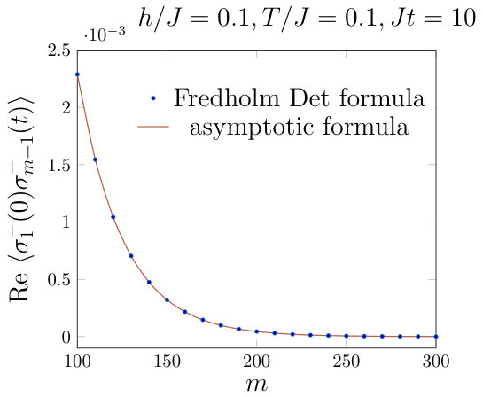 Figure 1
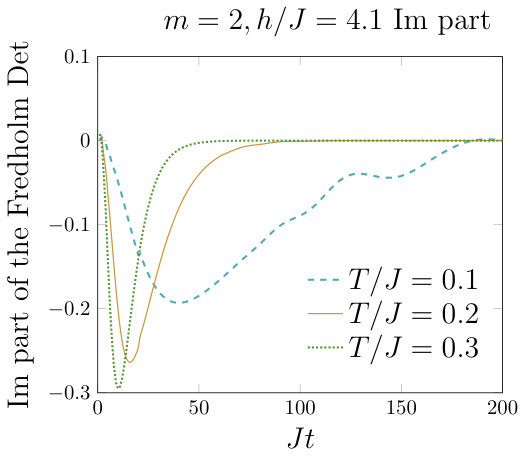 Figure 2
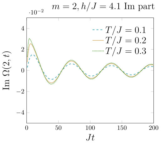 Figure 3
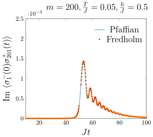 Figure 4
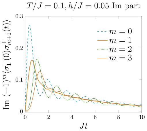 Figure 5
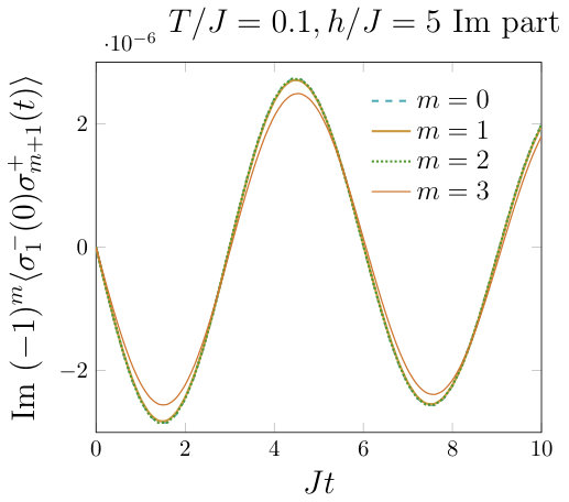 Figure 6
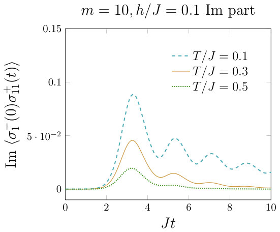 Figure 7
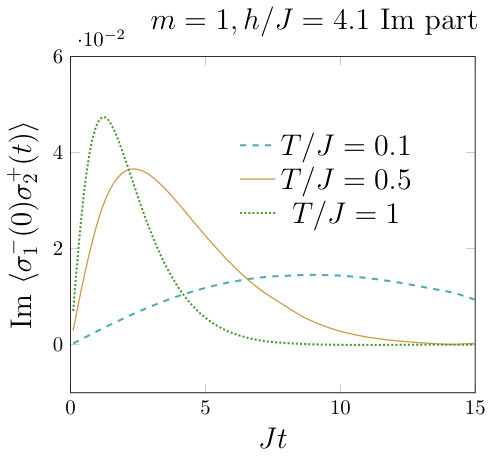 Figure 8
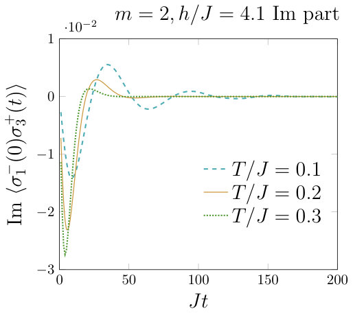 Figure 9
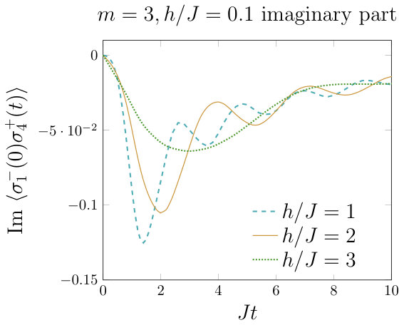 Figure 10
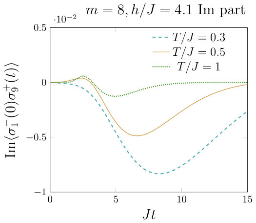 Figure 11
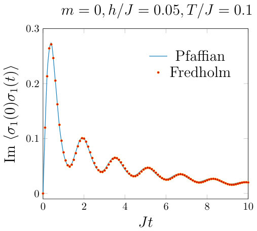 Figure 12
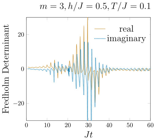 Figure 13
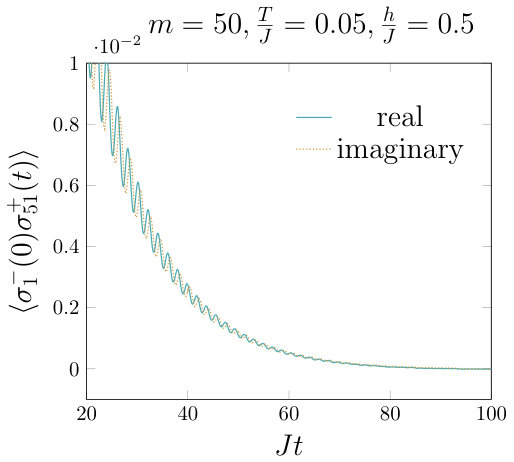 Figure 14
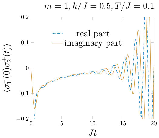 Figure 15
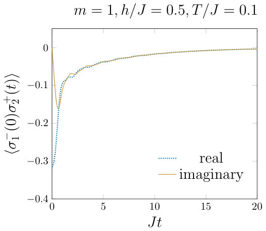 Figure 16
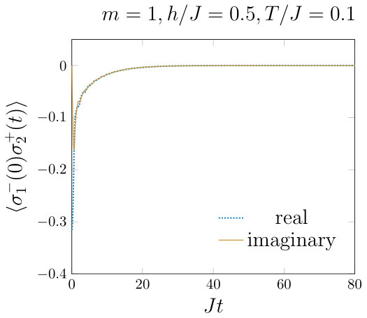 Figure 17
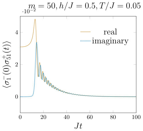 Figure 18
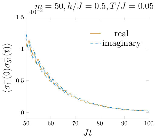 Figure 19
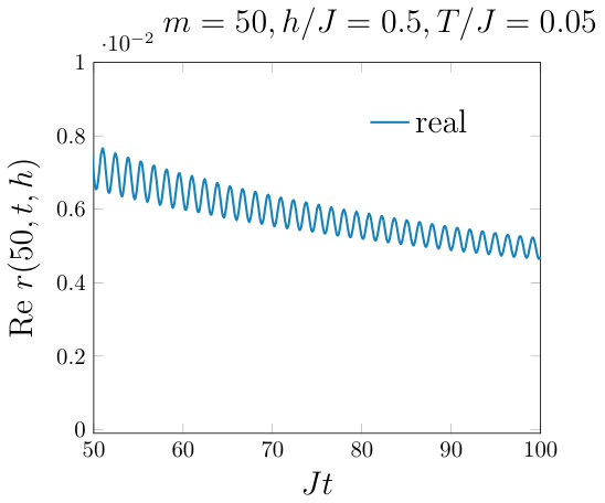 Figure 20
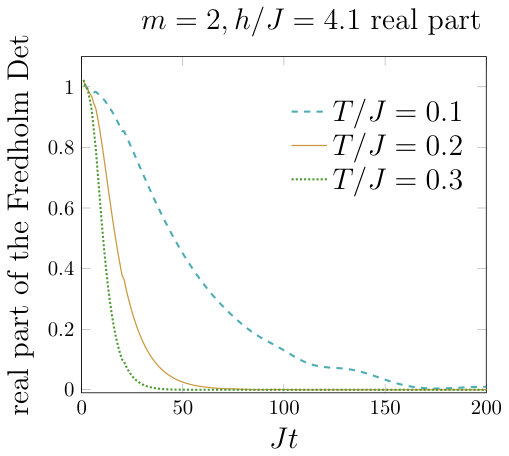 Figure 21
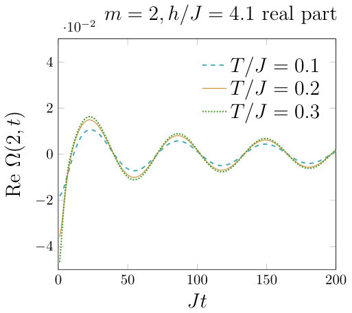 Figure 22
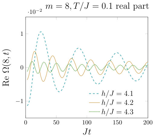 Figure 23
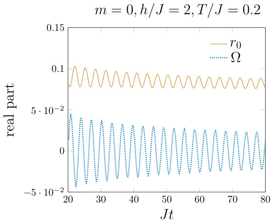 Figure 24
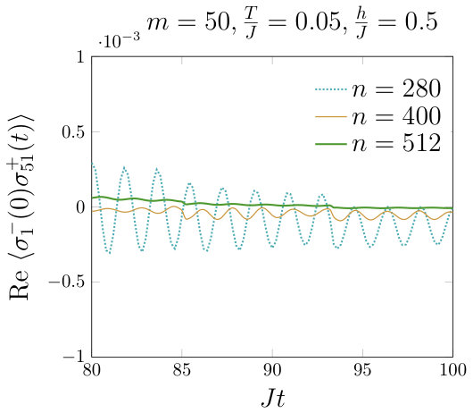 Figure 25
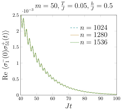 Figure 26
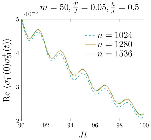 Figure 27
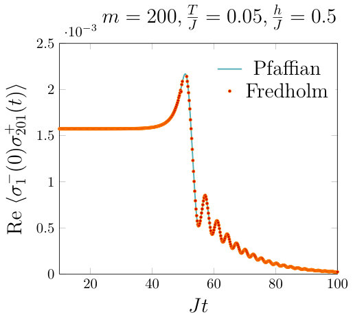 Figure 28
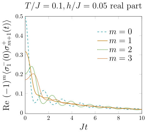 Figure 29
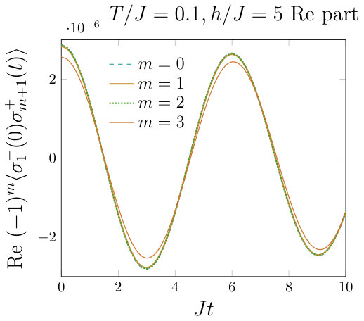 Figure 30
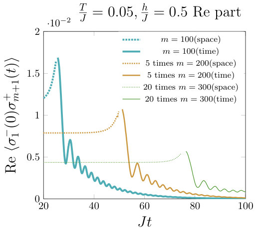 Figure 31
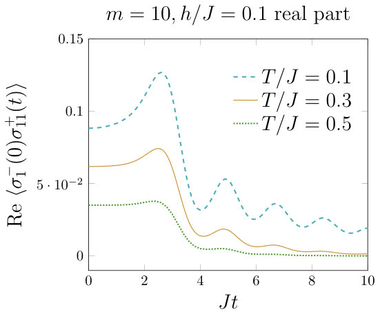 Figure 32
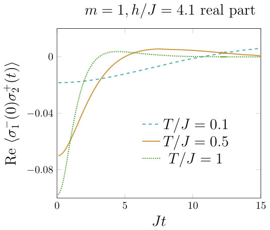 Figure 33
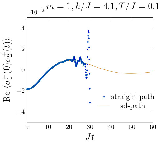 Figure 34
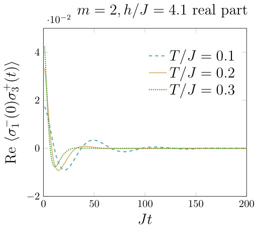 Figure 35
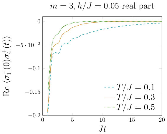 Figure 36
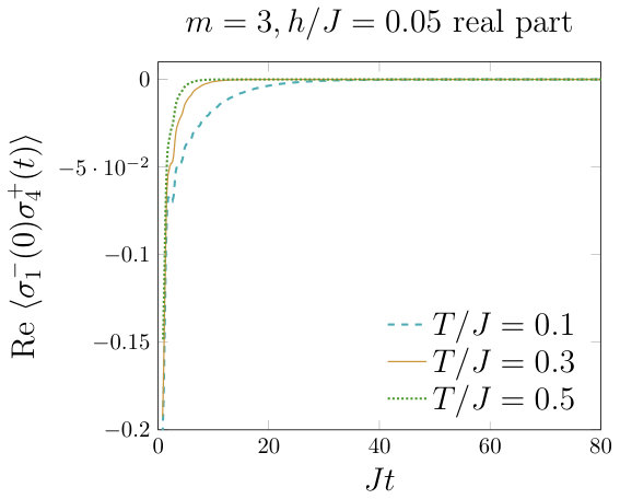 Figure 37
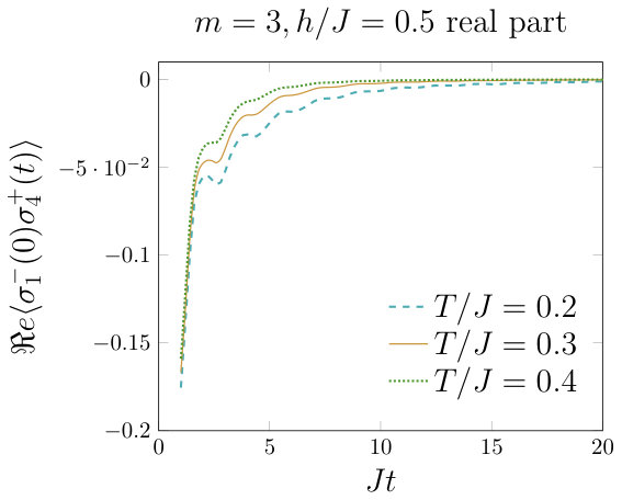 Figure 38
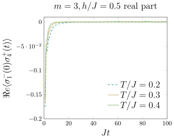 Figure 39
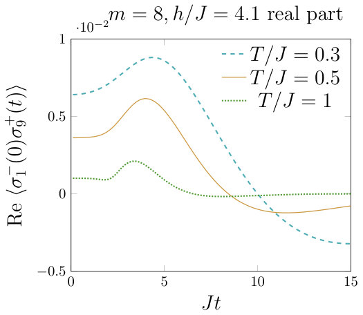 Figure 40
| T | exact | |||
|---|---|---|---|---|
| 0.1 | -0.34556050 | -0.31549848 | -0.31547691 | -0.31547744 |
| 0.5 | -0.32068971 | -0.30676642 | -0.30675704 | -0.30675704 |
| 1 | -0.28351570 | -0.27640356 | -0.27639925 | -0.27639925 |
| T | m=0 | m=1 | m=2 | m=3 |
|---|---|---|---|---|
| 0.1J | 0.4920331867 | -0.3178821170 | 0.2022244472 | -0.1710719802 |
| 0.4920331808 | -0.3178821255 | 0.2022244549 | -0.1710719748 | |
| 0.5 J | 0.4917867108 | -0.3094178153 | 0.1915980505 | -0.1508065219 |
| 0.4917866789 | -0.3094178186 | 0.1915980506 | -0.1508065200 | |
| J | 0.4910914106 | -0.2793621277 | 0.1561766021 | -0.1020132729 |
| 0.4910913226 | -0.2793621160 | 0.1561766025 | -0.1020132730 | |
| 5 J | 0.4953703567 | -0.0961933456 | 0.0185079888 | -0.0036065564 |
| 0.4953703745 | -0.0961933456 | 0.0185079891 | -0.0036065569 |
| T | m=0 | m=1 | m=2 | m=3 |
|---|---|---|---|---|
| 0.1J | 0.0186123689 | -0.0183512823 | 0.0176076636 | -0.0164562085 |
| 0.0186123688 | -0.0183512823 | 0.0176076634 | -0.0164562090 | |
| 0.5 J | 0.0765154951 | -0.0704244629 | 0.0563287894 | -0.0402407959 |
| 0.0765154951 | -0.0704244629 | 0.0563287892 | -0.0402407964 | |
| J | 0.1186618941 | -0.0983455062 | 0.0624189803 | -0.0338002579 |
| 0.1186618940 | -0.0983455062 | 0.0624189800 | -0.0338002583 | |
| 5 J | 0.3181814080 | -0.0830610673 | 0.0160102135 | -0.0029751725 |
| 0.3181814073 | -0.0830610672 | 0.0160102133 | -0.0029751730 |
| m=5 | m=6 | m=7 | m=8 | m=9 | m=10 | m=20 | |
|---|---|---|---|---|---|---|---|
| Extrapolated | -0.132188 | 0.119687 | -0.111465 | 0.103810 | -0.0982175 | 0.0929276 | 0.0659939 |
| Exact | -0.132195 | 0.119691 | -0.111467 | 0.103807 | -0.0982084 | 0.0929116 | 0.0657593 |
Peer Reviews
No public reviews on file for this paper yet. If you reviewed it on a platform where reviews are public (OpenReview, ICLR, NeurIPS, ICML), you can paste yours below so the community can read it here.
Videos
No videos yet. Explain this paper in a talk, walkthrough, or lecture? Add one.
Equilibrium dynamics of the XX chain
Frank Göhmann
Fakultät für Mathematik und Naturwissenschaften, Bergische Universität Wuppertal, 42097 Wuppertal, Germany
Karol K. Kozlowski
Univ Lyon, ENS de Lyon, Univ Claude Bernard, CNRS, Laboratoire de Physique, F-69342 Lyon, France
Jesko Sirker
Department of Physics & Astronomy, University of Manitoba, Winnipeg, Manitoba, Canada R3T 2N2
Junji Suzuki
Department of Physics, Faculty of Science, Shizuoka University,Ohya 836, Suruga, Shizuoka, Japan
Abstract
The equilibrium dynamics of the spin- XX chain is re-examined within a recently developed formalism based on the quantum transfer matrix and a thermal form factor expansion. The transversal correlation function is evaluated in real time and space. The high-accuracy calculation reproduces several exact results in limiting cases as well as the well-known asymptotic formulas obtained by the matrix Riemann-Hilbert approach. Furthermore, comparisons to numerical data based on a direct evaluation of the Pfaffian as well as to asymptotic formulas obtained within non-linear Luttinger liquid theory are presented.
I Introduction
An increasing knowledge has been acquired on the correlation functions of the simplest models which are integrable in the sense of the Yang-Baxter relation. The vertex operator approach (VOA) has definitely triggered the recent advance Jimbo and Miwa (1995). It enables us to evaluate ground state correlation functions, for instance, of the XXZ chain in the antiferromagnetic regime in a vanishing magnetic field. A multiple-integral formula for the reduced density matrix has been derived naturally within this framework Jimbo et al. (1992). The evaluation of the two- and four-spinon contributions to the dynamical structure factor of the massive XXZ chain Bougourzi et al. (1998); Abada et al. (1997) and the four spinon ones in the XXX limit Caux and Hagemans (2006) were important outcomes of this method.
A complementary approach to the analysis of ground-state correlation functions of the XXZ chain starts with its algebraic Bethe ansatz solution. It utilizes the solution of the quantum inverse problem Kitanine et al. (2000a) and a special determinant formula for the scalar product of on-shell and off-shell Bethe vectors Slavnov (1989). The algebraic Bethe ansatz approach successfully confirmed Kitanine et al. (2000b) the multiple-integral formula for the density matrix obtained within the VOA. It properly takes into account the effect of a finite magnetic field in the symmetry direction of the chain. This approach can be also used to derive and analyze form factor series for dynamical correlation functions in the thermodynamic limit Kitanine et al. (2009); Kitanine et al. (2011a, b); Kitanine et al. (2012); Dugave et al. (2015); Kozlowski and Maillet (2015); Kozlowski (2018). These developments culminated in the extraction, on the basis of exact and first principle calculations, of the long-distance and large-time asymptotic behavior of two point functions in the XXZ chain at zero temperature Kozlowski (2019a). Also, it was possible to grasp on exact grounds, the full structure of the edge singularities of the spin structure factors and spectral functions in this model Kozlowski (2019b).
In a parallel development, field theoretical approaches have been extended to include non-linearities in the spectrum Imambekov and Glazman (2009); Imambekov et al. (2012). It has been argued that using non-linear Luttinger liquid theory is crucial to obtain proper universal results for threshold singularities in spectral functions and for the long time asymptotics of dynamical correlation functions. For integrable lattice models, in particular, a combination of non-linear Luttinger liquid theory and Bethe ansatz has allowed to derive parameter-free results for edge singularities and high-energy tails of spin structure factors and spectral functions Pereira et al. (2006, 2007, 2008, 2009). Of particular relevance in the present context are results for the asymptotics of the dynamical longitudinal spin-spin correlation function Karrasch et al. (2015) and the transverse spin-spin structure factor Karimi and Affleck (2011) for the XXZ chain at low but finite temperatures. These results play the same role for dynamical correlations as the well-known conformal field theory formulas do in the static case. In contrast to the latter, however, a verification of the asymptotic formulas based on a fully microscopic calculation is so far lacking in the dynamical case at low but finite temperature.
It has been observed that the simplest multiple integrals representing the reduced density matrix of short sub-segments of the XXZ chain factorize Boos and Korepin (2001); Boos et al. (2003); Sakai et al. (2003); Boos et al. (2004, 2005). The algebraic structure of the ground state expectation values of all finite-range operators was finally understood with the discovery of a ‘hidden Grassmann structure’ on the space of such operators in Boos et al. (2007a, b, 2009). While the structure turned out to be relevant for the analysis of the short-range correlation functions Sato et al. (2011); Miwa and Smirnov (2019), the form factor series seem to be more efficient in analyzing the long time, large distance behavior of the two-point functions. The microscopic verification Kitanine et al. (2011a); Kozlowski and Maillet (2015) of the predictions of conformal field theory Cardy (1986) for the XXZ chain is an important application.
Thanks to the similarity in the structure of the row-to-row transfer matrix of the six-vertex model and the quantum transfer matrix (QTM) of the XXZ chain Klümper (1993), many results for ground state correlation functions of the XXZ chain could be generalized to finite temperatures. This concerns in the first place the multiple-integral representation for the reduced density matrix of sub-chains Göhmann et al. (2004); Göhmann et al. (2005a, b). The multiple integrals factorize even at finite temperatures Boos et al. (2006, 2007c, 2008), which finds its explanation again in the hidden Grassmann structure Jimbo et al. (2009). Moreover, for the static two-point functions at finite temperature so-called thermal form-factor expansions, involving form factors of the QTM, were introduced and studied in Dugave et al. (2013, 2014, 2016). As an interesting outcome we mention the evaluation of the static two-point correlation functions in the low-temperature limit in terms of higher particle-hole excitations Dugave et al. (2016). They were conjectured to correspond to the two-, four- and six-spinon contributions in the VOA.
As compared to the ground-state case, the inclusion of the time dependence into the thermal form factors series for the two-point functions requires slightly more thought. It was realized in Sakai (2007) that the solution to the inverse problem for the QTM has to be adopted for this purpose. By combining the lattice realization of the two-point functions suggested in Sakai (2007) with the thermal form factor expansion of Dugave et al. (2013), we recently proposed Göhmann et al. (2017) a new scheme for the explicit evaluation of dynamical correlation functions of quantum spin systems in thermal equilibrium. As a first test for the validity of the new scheme, we re-derived the well-known formula Niemeijer (1967) for the longitudinal equilibrium correlation function of the spin- XX chain. We also obtained a novel thermal form factor series for the transversal two-point correlation function which will be analyzed in this work.
It may seem rather amazing that for a simple model as the XX chain, whose Hamiltonian can be expressed in terms of non-interacting spinless Fermions Lieb et al. (1961), the calculation of its transverse dynamical two-point function at finite temperature still poses interesting questions. It is considerably harder than the longitudinal case, because the two-point function is non-local in terms of the Jordan-Wigner Fermions. Consequently, we are facing the problem of evaluating large determinants. Analytic studies are therefore mainly restricted to the case where each matrix element has a simple structure so that the Szegö theorem McCoy et al. (1971); Brandt and Jacoby (1976) can be applied. Results at finite temperatures, that were obtained within approaches based on the use of Fermions, comprise asymptotic formulae for high temperatures Brandt and Jacoby (1976); Perk and Capel (1977) as well as the numerical evaluation for finite open systems. The latter seems most efficient if the correlation function for a finite length chain is represented in terms of a Pfaffian of two-point functions of auxiliary Fermions Derzhko and Krokhmalskii (1997); Derzhko et al. (2000). Fermion algebra and generalized Wick theorem lead to an important consequence in the XY chain and its limit, a set of nonlinear difference-differential equations. See Perk (1980); McCoy et al. (1983); Perk et al. (1984); Perk and Au-Yang (2009) and references therein.
A completely different route to the evaluation of the transverse dynamical two-point functions was taken in Colomo et al. (1993). Following the strategy of Korepin and Slavnov (1990) the authors of Colomo et al. (1993) used the coordinate Bethe ansatz to derive a Fredholm determinant representation of the correlation function in the thermodynamic limit. The integral operator in the Fredholm determinant is of integrable type Korepin et al. (1993). This formulation was then directly suitable for an asymptotic analysis at long times and large distances by means of an associated matrix Riemann-Hilbert problem amenable to a ‘non-linear steepest descent method’ Deift and Zhou (1992). In Its et al. (1993) it was shown that the long time, large distance behavior of the two-point function for a fixed ratio in a weak magnetic field () goes like . The explicit expressions for and were obtained in the space-like () and time-like () asymptotic regimes. The result was subsequently extended to strong magnetic field () Jie (1998).
This is one of three companion papers in which we revisit the problem of the evaluation of the transversal two-point function at finite temperatures. Our starting point will be the novel thermal form factor expansion for that was derived in a previous communication Göhmann et al. (2017). In Göhmann et al. (2019a, b) we study two different aspects of asymptotic analysis: On the one hand, the high-temperature analysis for all times and all distances and, on the other one, the evaluation of the amplitude in the space-like regime at weak magnetic field (). In this communication, we shall concentrate on the numerical evaluation of the series. We will remind the reader in Section II that the form factor series can be neatly re-summed in terms of a Fredholm determinant different from the one in Colomo et al. (1993). The kernel of the integral operator that defines the Fredholm determinant is a strongly oscillating function for large values of and . We shall demonstrate that, nevertheless, the idea presented in Bornemann (2010) of a direct evaluation of the determinant can be applied, if combined with an appropriate choice of the integration contour in the complex plane. Then the real time evaluation can be performed in a stable manner until rather large times . Consequently, we are able to numerically check the asymptotic results of Its et al. (1993); Jie (1998). We are also able to suggest a higher-order correction for from our numerical analysis. The advantage of the method of numerical evaluation proposed in this work is that it works directly in the thermodynamic limit and is free of finite size effects.
The paper is organized as follows. In Section II, we start from a brief review of the results in Göhmann et al. (2017) and then derive the novel Fredholm determinant representation of the transverse correlation function. We will discuss the analytic properties of the functions occurring in the determinant in Section III. The steepest-descent paths in the space-like and time-like regimes will be explained. They are crucial for the numerics, especially in the large-time dynamics and for the long-distance correlations. Based on these preparations, we present the result of our numerical analysis in the massive phase in Section IV. The kinematic poles will become important at a later stage, and we shall argue how they can be treated numerically. The situation becomes more complicated in the massless phase due to the presence of Fermi points on the real axis. This will be discussed in Section V. In Section VI numerical data are presented showing the difference in the oscillation amplitudes of correlation functions at odd and even distances. These differences are then explained based on asymptotic results obtained within non-linear Luttinger liquid theory. A comparison with the analytic predictions based on the Fredholm determinant representation derived in Colomo et al. (1993) is given in Section VII. Thanks to the high-precision calculation, we identify a higher order correction in the massless phase. In Section VIII we compare the new numerical scheme proposed here and a previously existing method based on the Pfaffian representation. We summarize our results and point out perspectives in Section IX. Some of the technical details as well as a comparison with the exact static values are supplemented in several appendices.
II A representation of the transverse correlation function by a Fredholm determinant
We consider the spin- XX chain,
[TABLE]
with periodic boundaries in the thermodynamic limit . We assume the strength of the spin-spin interaction and the Zeeman magnetic field to be positive. The model has two phases in its ground state phase diagram, a critical phase (low ) with finite magnetization that depends of the value of , and a massive phase (high ) in which the magnetization is saturated to its maximal possible value . The two phases are separated by the critical field
[TABLE]
The quantity of interest in this work is the transverse correlation function
[TABLE]
We shall consider it as a function of distance and time that depends parametrically on and and on the temperature . The subscripts will often be suppressed below.
We divide the - space-time plane into two regimes: the space-like regime with and the time-like regime with , where
[TABLE]
We shall see that the qualitative behavior of the transverse correlation function falls into 4 categories: massive time-like, massive space-like, massless time-like and massless space-like. Our aim is to understand the different categories quantitatively based on the QTM method.
The application of the QTM method and the derivation of a thermal form factor expansion for the transverse correlation function (3) of the XX model was described in detail in Section 3.5 of Göhmann et al. (2017). We give a brief summary of the result obtained there in Appendix A.
II.1 A representation by a Fredholm determinant
In our previous work Göhmann et al. (2017) we expressed the integrals in the thermal form factor series in terms of rapidity variables (see (29)). This is natural for integrable systems in general, but for the numerical study presented here, it turns out to be more convenient to switch to momentum variables . Then the one-particle dispersion takes its familiar functional form
[TABLE]
By the common abuse of notation we use the same symbol to denote the energy as a function of the momentum or rapidity variables. The substitution in (29) with according to (26) then leads to
[TABLE]
where is defined in (28),
[TABLE]
and (respectively ) is the boundary value as approaches from above (respectively below). We call the hole momenta and the particle momenta. The contour is a straight line in the massive phase, . Similarly, is a contour just below the real axis. When , the contours will be slightly deformed in order to avoid the Fermi points111The Fermi momentum with the proper dimension will be introduced later in Section VI. (defined by ) as shown in Figure 1. The contours and are the images of and (see Appendix A) under the transformation .
Using a technique developed in Korepin and Slavnov (1990) we can rewrite (5) as an explicit factor times a Fredholm determinant of a special form. For this purpose, let us prepare some notations in advance,
[TABLE]
where
[TABLE]
We further define integral operators,
[TABLE]
The operator is obviously a one-dimensional projector. After these preparations, by a calculation very similar to that in Göhmann et al. (2019a), we obtain the following formula.
Theorem**.**
The transverse correlation function of the spin- XX model can be represented using a Fredholm determinant that involves the integral operator ,
[TABLE]
The symbol means the Fredholm determinant where the integral operator is acting on functions supported on .
Equation (10) is a novel analytic expression representing the transverse dynamical correlation function (3) of the infinite system at finite temperatures. In recent years it has become increasingly clear Bornemann (2010) that Fredholm determinants can be very efficiently evaluated numerically by simply approximating them by determinants of finite matrices, very much like integrals are approximated by finite sums. The numerical error decreases with the number of discretization points. It has been estimated for kernels with various analytic properties in Bornemann (2010).
When we evaluate (10) numerically, we are considering the kernel as a function of the momentum variables that depends parametrically on distance and time . When and become large, the kernel function becomes a rapidly oscillating function of the momentum variables on the contour . This affects the numerical accuracy of the calculation in a similar way as in the case of integrals over rapidly oscillating functions. As we shall see, the cure to this problem as well is similar as in the case of integrals over rapidly oscillating functions. We have to deform the integration contour in the complex plane into a saddle point contour. Since we are dealing with meromorphic functions with infinitely many poles the deformation is an intricate issue. This will be, on a technical level, the main subject of the discussions in the following sections.
We would like to remark that belongs to the class of integrable integral operators Korepin et al. (1993). This is easily seen if we rewrite its kernel in the following form,
[TABLE]
For integrable integral operators there exist powerful tools in order to analyze the asymptotic behavior analytically Deift and Zhou (1992). A representation of the correlation function (3) involving a Fredholm determinant with a similar but manifestly different kernel, which belongs to the family of integrable integral operators as well, was analyzed in Its et al. (1993). The leading terms of the large space and time asymptotic behavior of the transverse correlation function of the XX model have been successfully derived from that representation. Here, however, we are interested in a quantitative study on an arbitrary space scale and time scale.
III The analytic properties of integrands and the steepest
descent paths
The contours are optimal choices in the static limit. As time evolves, the phase factors bring instability and we eventually need to deform the contours for a reliable calculation. One may encounter singularities of the integrands during the deformation. We thus have to find a balance between the advantage of reducing the instability from and the cost of passing through many singularities of the integrands. Below we shall discuss the analytic properties of the integrands and the optimal choice of integration paths.
III.1 The saddle points and the steepest descent paths
We need to take account of the steepest descent paths for in the asymptotic region . The locations of saddle points for the system in the space-like regime are qualitatively different from those for the system in the time-like regime. On the other hand, they do not depend on whether the system is in the massive or in the massless phase.
III.1.1 The space-like regime
The saddle points in the space-like regime lie at
[TABLE]
The red points in Figure 2 denote them. The dashed curve corresponds to the loci of points such that \operatorname{Im}\bigl{(}u_{m,t}(p)\big{)}=\operatorname{Im}\big{(}u_{m,t}(p_{+})\big{)}, and the shaded region satisfies . Thus, the steepest descent path for the hole momentum passes through horizontally and never enters into the shaded region. We have an upside-down figure for the path of the particle momentum which passes through , as it has the conjugate phase . As a result, the optimal path for the hole (particle) momentum in the space-like regime is similar to (): it stays above (below) the real axis.
III.1.2 The time-like regime
In this regime the saddle points are on the real axis,
[TABLE]
They are depicted by red dots in the right panel of Figure 2. The shaded region indicates . Thus, for the hole momentum, the steepest descent path runs through and , while staying inside of the un-shaded region. Accordingly, it cannot stay above the real axis, but passes below the real axis for . The figure for the particle momentum is obtained by turning the figure for the hole momentum upside down.
III.2 The analyticity of and
We only have to know () in (II.1) as functions of in the upper (lower) half plane in the space-like regime. As was already discussed, one needs to continue them analytically into the whole complex plane in the time-like regime. The analytic properties turn out to be quite different for the massless () phase and for the massive () phase.
III.2.1 The massive regime
We set
[TABLE]
so that
[TABLE]
We further define “upper roots” and “lower” roots by
[TABLE]
so that and .
The roots closest to the real axis are q^{u}_{0}=i\operatorname{arch}\bigl{(}\frac{h}{4J}\bigr{)} and .
The following analytic properties of are derived in B.
Lemma 1**.**
*The function has
i) simple poles at in the upper half plane,
ii) double poles at in the lower half plane,
iii) simple zeros at in the lower half plane.
There is a strip including the real axis which is free of zeros and poles (of width 2\operatorname{arch}\bigl{(}\frac{h}{4J}\bigr{)}).*
Figure 3 (left panel) illustrates the situation. The red crosses represent single poles, while blue triangles are double poles. The circles denote the single zeros.
The zeros and poles for are obtained by taking the mirror image with respect to the real axis.
Note that the width of the analytic strip is independent of the temperature in the massive phase. Once a finite magnetic field is imposed, the width stays finite. Thanks to this fact, the evaluation of the correlation function is simpler in the massive regime.
III.2.2 The massless regime
We denote by , the (right) “Bethe roots”, which are identical to the in eq. (14). Note that . The (left) “Bethe roots” are defined by .
In B we show that () has the following analytic properties.
Lemma 2**.**
*The function has
i) simple poles at and at () in the upper half plane,
ii) a simple pole at and a simple zero at on the real axis,
iii) double poles at and at () in the lower half plane,
iv) simple zeros at and at ().
The zeros and poles of are obtained by taking the mirror image w.r.t. the origin.*
The massless case is illustrated in the right panel of Figure 3. The differences and become as . Thus, singularities will approach towards the real axis as and the choice of the contours becomes difficult. This poses a technical problem in the massless regime.
IV Numerical study of the massive regime
In this and in the next sections we present the results of our study of the transverse correlation function based on the numerical evaluation of (10). We follow the proposal in Bornemann (2010) and evaluate the Fredholm determinant by a Gauss-Legendre integration with discrete points.
We shall start from the simpler case . In this case the Fermi points are away from the real axis. Thus, we can separately treat two technical problems, how to deal with the Fermi points and how to deal with the steepest descent path.
IV.1 The space-like regime
In spite of having discussed the steepest descent path above, we can use simple straight integration contours in order to produce accurate results, as long as in this regime. In order to demonstrate this, we first consider the static limit where many results are available. The exact static short-range correlation functions at arbitrary and were obtained, e.g., in Boos et al. (2008) (for the XXZ model in general). We compare them with the static results obtained from (10) in C. The results match with reasonable precision. We have to choose, of course, the appropriate number of discretized points to achieve agreement. For example, fixing and we find
[TABLE]
Thus, we can say that with , eq. (10) practically reproduces the exact value. For larger segments, some indirect evidence is presented in D. Encouraged by this success, we adopt the straight contours in the space-like regime as they are conveniently simple for the calculation. Indeed, they produce accurate results even beyond .
Figures 4 and 5 show examples for , and for various . The horizontal axes indicate . Although the space-like regime is limited to when and when , the straight contours produce stable values even after .
The real part stays almost flat in the space-like regime. This can be better seen in the case of in Figure 5. The amplitude is enhanced around .
For larger values of (typically ), we need to adopt contours which take into account the steepest descent paths. The saddle points in eq. (12) are located away from the real axis, and we shift the contour ( ) to a straight line passing though (). The integration contours cross poles of and if , which is clearly seen in Figure 3 (left). This modifies our formula (10) slightly, following the argument in Dugave et al. (2016), which will be summarized in E for the reader’s convenience.
IV.2 The time-like regime
The calculation with the straight integration contours gradually becomes unreliable for larger . An example is given in Figure 6.
We thus deform the contours in the time-like regime. The most naive choices for the hole momentum () and for the particle momentum may be the ones depicted in Figure 7, which respect the steepest descent paths discussed in Section III.1.
The paths are determined only by the phases and . One, however, needs to be careful: Since and are swapped, there appears an additional term in ,
[TABLE]
due to a pole of at . Here denotes the red path in Figure 7. As we interpret ( respectively ) as the momentum of a hole ( respectively a particle), we refer to the singularity as the kinematic pole in analogy with scattering theory. Consequently, the kernel of the integral operator contains a term
[TABLE]
This becomes very large for if and makes the calculation again unstable. We thus choose the red contour in Figure 7 for the variables while we adopt a straight contour for the variable such that and for .
Still, there is a problem in dealing with the intersection points . We simply exclude them from the set of discretized sampling points in the integrals over the variable.
After the above modification and by increasing the number of sampling points for the Fredholm determinant (, typically), a large scale calculation is possible. As an illustration, the plots for are shown in Figure 8.
One immediately notices the very long period oscillation. This may be attributed to the oscillatory behavior of of which the period seems to depend only weakly on temperature (Figure 9).
The amplitude of decreases slowly in time and the decay of the amplitude of the correlation functions mainly comes from that of the Fredholm determinant, c.f. Figure 10, especially for higher .
Unlike on temperature, the period of oscillation obviously does depend on the magnetic field, and it grows as approaches (Figure 11). It may be easier to check this by looking at the imaginary part of (cf. right panel).
The oscillatory period of is easily understood in the asymptotic region and . A saddle point analysis yields
[TABLE]
Note that , and . Due to the asymmetry of the integrand in (II.1) for or , one can show that so that . On the other hand . Thus,
[TABLE]
and we can safely drop the first term in (IV.2). Thus, we are left with a single oscillating term and conclude that the period of the oscillation diverges as , for some constant , when . Note that is an exceptional point as the Fermi points pinch the real axis and the above argument is not valid.
V Numerical study in the massless regime
The existence of Fermi points on the real axis makes the evaluation technically more involved than in the massive case. This is due to the fact that the Fermi-point singularity problem and the steepest-descent path problem are coupled. The situation is slightly simpler in the space-like regime from which we start our consideration.
V.1 The space-like regime
We again transform to a straight contour in the upper (lower) half plane for the hole (particle) momentum if is not too big. By this deformation, in contrast to the massive case, we inevitably pick up the contribution from the Fermi points. This modification can be treated in a similar manner as the contributions of the other poles, shortly commented on at the end of Section IV.1 on the massive phase. The details are explained in E. We choose a straight contour for . Although the choice of is in theory arbitrary, in practice one should not take it too small. Table 1 illustrates this with the examples of , and for various choice of . The rightmost column gives the exactly known static values.
This can be easily understood as the contour passes near the singularities of (at ) or (at ). Hence, too small values of spoil the numerical accuracy.
With suitable choices of we can again adopt the straight line contours well beyond the space-like regime, see Figure 12.
The oscillation frequency in the time-like regime for small temperatures is given by the effective bandwidth in the Fermionic model, , and goes to zero as approaches as demonstrated in Figure 13.
For larger values of , is determined by the location of the saddle point (12) and one has to the take into account the pole contributions as described in E. Some numerical results will be supplemented later (cf. Section VIII).
V.2 The time-like regime
As in the massive phase, the straight integration contours fail to give reliable results as time evolves. Figure 14 shows an example.
We thus utilize the steepest descent paths. The existence of Fermi points on the real axis makes the situation more involved than in the massive case. At the same time, one must pay attention to the singularities of . The choice of the paths thus becomes a complicated technical issue, and we decided to summarize it in F.
By applying the prescription presented there, the result are now stable as shown in Figure 15, where we have chosen the same parameters as in Figure 14. The right panel represents the result up to , and the real part of decays to the order of .
Examples with slightly different parameters are given in Figure 16, showing again smooth behavior until they exhibit sufficient decay.
The fluctuation is enhanced at lower temperatures, where one has to be particularly careful. Independent calculations also suggest this. For example, the authors of Derzhko et al. (2000) calculated in the finite XX-chain (400 sites) using the Pfaffian representation. Their result does not converge numerically for various choices of around for (in the present normalization). The authors claim that this is due to a “boundary effect”. Our results using the Pfaffian representation of the correlation function, which we present in Section VIII, do not show such instabilities. This suggests that the observed instabilities are numerical in nature (a critical step is a numerically stable direct evaluation of the Pfaffian) and not related to boundary effects. In the framework of our QTM approach we are dealing with an infinite size system from the beginning so that boundary effects are certainly absent. Nevertheless, a similar instability is observed at lower temperatures. We examined each factor in (10) and found that the instability mainly comes from the Fredholm determinant (Figure 17).
In order to achieve higher accuracy in the evaluation of the Fredholm determinant, we increase the number of discretization points. We defer the discussion of the right choice of to G. With suitable values of , we are able to perform a precise evaluation of on a longer time scale. An example is given in Figure 18. The right panel presents a zoom of the curves for large . This exhibits a slowly decaying oscillating pattern.
VI Even-odd effect
There are similarities and differences between the transverse correlator in the massive and in the massless regime, as we observed above. We comment on one more difference which seems to have been overlooked in past publications: the even-odd effect. By this we mean a drastic suppression of the oscillation amplitude of for being odd and for small . The plots in Figure 19 present examples in the massless phase.
On the other hand, this even-odd difference is not observed in the massive case. See Figure 20.
Our formula consists of several factors (10). The behavior of is the same for odd and even. We numerically find that in the massless case the oscillation phase of and that of the Fredholm determinant part almost cancel each other and that this results in the monotonous time evolution for odd . By way of contrast the two contributions do not cancel each other for even or in the massive case.
The even-odd effect in the massless case can be explained straightforwardly within non-linear Luttinger liquid theory. A first step in the derivation of the long time asymptotics of the transverse spin-spin correlation function of the XXZ chain is a Jordan-Wigner transformation onto spinless Fermions with annihilation operator . Next, the dispersion is linearized around the Fermi points with where is the lattice constant. After using the standard Bosonization identities, this approach then allows to calculate the low-energy contributions to the transverse spin-structure factor which are located at momentum and where is the magnetization per site. Standard Bosonization thus predicts that there are two low-energy contributions to the transverse spin-spin correlation function. At the XX point, the contribution from is dominant and is given for small temperatures by Karimi and Affleck (2011)
[TABLE]
Here is the sound velocity and denotes a small regularization parameter. Note, in particular, that for and standard Bosonization predicts a decay at long times. Furthermore, there is no part which oscillates in time at this level. To obtain the oscillating contribution one needs to keep—in addition to the Fermi point contributions covered by standard Bosonization—also the saddle point contributions which appear at real momenta for , see eq. (13) 222 Here the momentum has a proper dimension . Doing so leads to non-linear Luttinger liquid theory. In the XX case, the theory is particularly simple because the saddle point and the Fermi point contributions do not interact with each other. We now use the extended ansatz where denotes a particle near the saddle point. It is then a fairly straightforward calculation to show that the additional saddle point contribution is Karimi and Affleck (2011)
[TABLE]
We are interested here in understanding the asymptotic behavior in the time-like regime for and . In this limit we have and we can approximate the propagator for the high-energy particle by . Putting together the two contributions (17) and (18) for this case we arrive at
[TABLE]
with some unknown amplitude . In the zero temperature limit, in particular, eq. (19) predicts that the correlation function asymptotically consists of a uniform part which decays as and part which decays as and oscillates with frequency .
Crucially, the oscillating part contains a factor . This means that for () the oscillating contribution is absent if the spatial distance in the two-point correlation function is odd!
To check the predictions of Eq. (19) we present in Figure 21 low-temperature numerical data for the auto- and nearest-neighbor correlation function at (left panel) and (right panel).
¿From the log-log plot it is clear that for the correlation functions decay following a power law in time for all cases. For () the autocorrelation shows oscillations while the nearest-neighbor correlation function does not whereas both are oscillating for . A comparison with eq. (19) using the amplitudes of the uniform and the oscillating part as fitting parameters confirms that the long time behavior is described by the non-linear Luttinger liquid result and that the factor is indeed the reason for the observed even-odd effect at zero magnetic field. Finally, we note that higher order corrections to eq. (19) do exist, i.e. terms which decay faster than at . Such terms are responsible for the remaining small oscillations observed in the nearest-neighbor correlation function at zero field.
VII Comparison with asymptotic formulae
Starting from a slightly different Fredholm determinant Its et al. Its et al. (1993) reformulated the problem of the asymptotic analysis of the transverse correlation function in terms of a matrix Riemann Hilbert problem. They obtained a closed expression for the leading terms of the asymptotic expansion of the transverse correlation function in and with a fixed direction s.t. at arbitrary and . The space-like regime (VII.1) corresponds to while the time-like one (23) does to . Subsequently their method was applied to the massive case in a PhD thesis by Jie Jie (1998). An interesting feature of our novel thermal form factor series (29) is that it is more suitable for the long time, large distance analysis in the space-like regime than the Fredholm determinant representation of Its et al. Its et al. (1993) in that the asymptotics can be easily extracted from the first term in the series. For this reason we can obtain the constant term in the asymptotic expansion which was heretofore unknown in the massless phase. In this section, we provide a quantitative comparison of the available asymptotic formulae with our numerical results.
VII.1 Space-like regime in the massless phase
Its et al. Its et al. (1993) use a Hamiltonian in (1) and provide formulae for the conjugate transversal correlation function
[TABLE]
By a unitary transformation and an adaption of parameters, it is related to ours by
[TABLE]
In the space-like regime of the massless phase their asymptotic formula translates into
[TABLE]
after properly recovering the exchange coupling . The constant was not explicitly calculated in Its et al. (1993). Within our framework it is not hard to reproduce this formula and to obtain an explicit expression for from eq. (29),
[TABLE]
where is an inverse image of , in (26). See Göhmann et al. (2019b) for details. We supplement convincing numerical support in Figure 22.
We have to adopt the steepest descent paths even in the space like regime for larger values of in order to achieve sufficient accuracy.
We assumed that the other poles (of ) are sufficiently away from in the above derivation. When , however, they accumulate towards the Fermi points, and we inevitably have contributions from them which are neglected in the above as exponentially small corrections. Their estimation is an interesting problem which we hope to discuss in the future.
VII.2 Time-like regime in the massless phase
The asymptotic formula of Its et al. (1993) becomes more involved in the time-like regime,
[TABLE]
with
[TABLE]
and
[TABLE]
The authors of Its et al. (1993) did not present the explicit form of ( in their notation) but commented that the higher-order correction modifies , where . We again use (21) and re-introduce . As is real-valued for positive , it is natural to consider the ratio
[TABLE]
In view of asymptotic analysis, depends on only through .
Based on our numerics (with ) we propose
Conjecture 1**.**
For fixed and , the ratio consists of both non-oscillating and oscillating parts,
[TABLE]
The non-oscillating part includes . The period of the oscillating part behaves as as , and its amplitude is also expanded by powers of .
We, however, do not have any estimate of the time scale when the above asymptotic form becomes valid. For example, let us look at for with in Figure 23.
The average value does not seem to saturate, which suggests that is yet to reach the region described by the asymptotic formula if . There is, however, a limitation on the range of , for numerical accuracy. We thus need to find other ways than dealing with . Intuitively, the smaller is, the shorter we have to wait until reaches “equilibrium”. Thus, we focus on the extreme case (the auto-correlation). To be precise, this corresponds to the direction and the direct application of the formula (23) may need justification. We however assume its validity in the following.
The real parts of are plotted in Figure 24 for with .
While \operatorname{Re}\bigl{(}r_{\rm non-osc}(0,t,h)\bigr{)} is still slowly decreasing for , it already seems to approach “equilibrium” for around . The amplitude of the oscillating part \operatorname{Re}\bigl{(}r_{\rm osc}(0,t,h)\bigr{)} seems to be very slowly decreasing. In order to examine this quantitatively, we fit for using the data for ,
[TABLE]
The sum of the first two terms in the right-hand side is identified with . The sub-leading terms agree with the remark by Its et al. Taking this for granted, the real part of is estimated as in Figure 25.
The plot suggests that the amplitude of stays constant, that is, . This is again consistent with the estimate by Its et al..
There are remarks. One notices that \operatorname{Re}\bigl{(}r(0,t,h)\bigr{)} for shows a discontinuity at . This is a numerical artifact due to inaccuracy: already reaches . Thus, it is too difficult to have precise control over the numerics. The oscillatory part remains observable after sufficiently long time (except for ). The origin of the oscillation can be attributed to that of . The comparison of the real parts of and is given in Figure 26 for .
We can easily check that their frequencies coincide. One expects from eq. (10) that is proportional to , but it is not so simple. The inverse power of in the kernel of the Fredholm determinant partially cancels the oscillation, and this may contribute to the non-oscillating part . The center of oscillation of is thus different from zero, while it is zero for .
VII.3 Consistency with the result from nonlinear Luttinger Liquid theory
Finally, we comment on the relation between the above analysis and the results from the continuum theory, (17) and (19). We shall neglect logarithmic corrections in and consider only the leading behavior. Let us start from the space-like case, and . One applies a Sommerfeld type argument to the integral in (VII.1) and finds
[TABLE]
This is consistent with (17) for small but finite and . Next consider the time-like case and . The integral in (VII.2) has different forms for and for ,333The symbol is defined in (13).
[TABLE]
Thus if , together with Conjecture 1 and relation (21), we conclude that
[TABLE]
One identifies the terms on the right hand side with the dominant and sub-dominant terms in (19) if . This condition is consistent with the asymptotic analysis as is small but finite. In view of (19), the third and fourth terms in (25) look irrelevant and may be attributed to the weak transient behavior which still exists. We however do not have a conclusive evidence.
The above result suggests that the meaning of the space-like and time-like regimes undergoes a change in the low-temperature limit, or, in other words, that the ‘light cone’ needs to be redefined. At elevated temperatures, it is defined by , while in the low- limit, it is defined by the Fermi velocity, . This means that the space-like regime becomes enlarged in the low-T limit and that it becomes more enlarged if the magnetic field is higher.
VII.4 Time-like regime in the massive case
A similar long time, large distance asymptotic formula for the massive case was proposed by Jie Jie (1998). Set
[TABLE]
Then Jie argued that444An obvious typo in the second term ( instead of ) is corrected.
[TABLE]
where \alpha=\pi-\arcsin\bigl{(}\frac{m}{4tJ}\bigr{)} and is defined in (VII.2). The coefficient is a smooth function of and . The explicit forms of and are too complicated to be reproduced here. We only remark that as . Thus, only the second term survives in this limit, and it results the long-period oscillation observed numerically. The ratio
[TABLE]
is plotted in Figure 27. It seems to reach a constant value as time evolves.
VIII Comparison with the Pfaffian representation
In this section we compare our results with results obtained by more conventional methods. Among them, the Pfaffian representation of the correlation function is the most well-established for the dynamics of the XX model. It deals with an open chain of sites. As the translational invariance is broken, we rather consider instead of (3) and typically center the two-point correlation function at . After a simple calculation using the Fermion algebra, one represents by the Pfaffian of an anti-symmetric dimensional matrix, see e.g. McCoy et al. (1971); Derzhko et al. (2000) for details.
For small and the two results, one obtained by our formalism and the other one by the Pfaffian method,555We refer the numerical calculation based on the Pfaffian representation of the correlation function as “the Pfaffian method” for short. match perfectly. See Figure 28 for the autocorrelation function for , , and .
One of the advantages of the present approach in comparison with the Pfaffian method lies in the fact that the distance appears as a mere parameter. This allows us to deal with large immediately. For illustration, the data for and , obtained from eq. (10) are plotted in Figure 29 for .666 As is large enough, we use the steepest descent method also in the space-like regime. It becomes inaccurate around and some points are omitted near in the plots.
As indicated above, the Pfaffian formulation deals with a finite-size system. In order to eliminate the boundary effects, one has to choose the system size , the spin distance and the time so that is satisfied. Here stands for the sound velocity. Thus, for and becoming larger, one has to deal with a larger-size matrix. It is fair to note that one also needs to increase the number of discretization points in the evaluation of the Fredholm determinant in order to keep the numerical precision for larger . An example is discussed in G. With these tunings and using a stable direct evaluation of the Pfaffian (instead of calculating it as the square root of the determinant), the two results coincide also for large and . An example with and is shown in Figure 30.
We stress, however, that the numerical error in the present scheme solely originates from the discretization and should be distinguished form the error due to the finite size effect explained above. In the former case the error was estimated in Bornemann (2010). For the type of kernel occurring in our Fredholm determinant the error decreases algebraically with the number of discretization points.
IX Summary and conclusion
In this communication we revisited the equilibrium dynamics of the XX chain. We employed a new scheme for the exact evaluation of correlation functions, based on the QTM and on a thermal form factor expansion. We rewrote the thermal form factor series for the transversal correlation function as an explicit factor times a Fredholm determinant. This representation was the starting point of our numerical analysis, for which we utilized a direct discretization of the determinant as suggested in Bornemann (2010). We demonstrated that the method yields high-precision results for the transverse correlation function for a wide range of time, distance, temperature and magnetic field, if we properly use the freedom in the choice of the integration contour involved in the definition of the Fredholm determinant. The algorithm works for long times and large distances, far in the asymptotic regime, where we could confirm all existing analytic results Its et al. (1993); Jie (1998) and could even provide an estimation of the next order correction from our numerical data. We also checked our results by comparing with a numerical evaluation of the correlation function using the Pfaffian representation. Furthermore, we were able to explain even-odd effects in the observed oscillations in the massless time-like regime by non-linear Luttinger liquid theory.
We naturally expect, based on the success of the numerical study here, that the novel Fredholm determinant representation also provides an appropriate starting point for the analytic study of the XX chain. Although we have just started the investigation in this direction, there is already evidence that this is indeed the case Göhmann et al. (2019a, b).
A most important issue, from our point of view, is a possible extension to a truly interacting system, the XXZ chain. A single Fredholm determinant representation does not seem to exist in this case. But the thermal form factor series exists in the interacting case as well and represents the transversal correlation function as a series of multiple integrals having certain analogies with a Fredholm determinant Göhmann et al. (2017). Our numerical investigation suggests that the first few terms of this series may already provide accurate estimates in appropriate limiting cases. We hope to report concrete results in future publications.
Acknowledgments. F. Göhmann acknowledges financial support by the (DFG) in the framework of the research group FOR 2316 ‘Correlations in Integrable Quantum Many-Body Systems’. K. K. Kozlowski is supported by the CNRS and by the ‘Projet international de coopération scientifique No. PICS07877’: Fonctions de corrélations dynamiques dans la chaîne XXZ à température finie, Allemagne, 2018-2020. J. Sirker acknowledges support by the DFG in the framework of the research group FOR 2316 ‘Correlations in Integrable Quantum Many-Body Systems’ as well as support by the National Science and Engineering Research Council (NSERC) of Canada. J. Suzuki is grateful for support by a JSPS Grant-in-Aid for Scientific Research (C) No. 15K05208, No. 18K03452 and by a JSPS Grant-in-Aid for Scientific Research (B) No. 18H01141.
Appendix A A previous result
In this appendix we recall a previous result, obtained in Göhmann et al. (2017), from which we have derived the theorem in Section II.
In Göhmann et al. (2017) we proposed a method for calculating dynamical correlation functions at finite temperature in integrable lattice models of Yang-Baxter type. The method is based on an expansion of the correlation functions as a series over matrix elements of a time-dependent quantum transfer matrix rather than the Hamiltonian. Staying with the example of the transverse correlation functions of the XX chain, the series is obtained, when we apply, in a slightly sophisticated manner, respecting the integrability of the original quantum chain Klümper (1993); Suzuki et al. (1990); Klümper (1992), a Suzuki-Trotter decomposition Suzuki (1985) to the exponential factors in (3). As a result, the correlation function is represented as a (properly normalized) partition function of an alternating vertex model acting on a fictitious space of size , where is the Trotter number. This partition function can be interpreted as a trace of a product of many staggered column-to-column transfer matrices, the quantum transfer matrices, with two local insertions corresponding two the two local operators , , whose correlation function is considered. Using the ‘solution of the quantum inverse problem’ corresponding to the staggered monodromy matrices appearing in the columns and expanding in terms of the eigenstates of the QTM the thermal form factor series is obtained.
In case of the XX chains all matrix elements and correlation lengths appearing in the series can be calculated explicitly and the sums over classes of excitations (one hole, two holes one particle, three holes two particles …) can be turned into integrals. The integrands are composed of a number of functions characteristic of the XX chain. In the first place there are momentum and energy of the one-particle excitations as functions of the rapidity variable,
[TABLE]
The other functions needed in order to write the form factor series are
[TABLE]
and
[TABLE]
The contours and in the definition of are such that tightly encloses , and itself simply surrounds the strip counterclockwise with two infinitesimal deformations at the Fermi rapidities defined by , , .
Employing all of the above notation the thermal form factor series for the transverse correlation function (3) can be written in the form
[TABLE]
Here we are using a contour which tightly encloses . Note that as compared to the formula given in Göhmann et al. (2017) we have introduced a few minor simplifications by calculating two of the integrals in our original formula explicitly (one is zero the other one a constant) and by absorbing a constant term into the definition of the function .
Appendix B The analytic properties of
We first consider the massive case and assume that . We take the integral over a closed rectangular contour (of infinite height and width ), including the real axis as the bottom part,
[TABLE]
Note that the integrand on the upper edge of the rectangle reduces to a constant and the contributions from left and right sides cancel each other. We thus have
[TABLE]
On the other hand, one can evaluate the integral directly by summing up the contributions from the branch cuts connecting and and the pole at ,
[TABLE]
Thus, we conclude
[TABLE]
By remembering (15), one verifies that the double zeros and double poles at cancel and that the single poles at survive if .
The argument for the case goes almost in parallel. This time we consider a closed rectangular contour in the lower half plane. Using a similar reasoning as above, we obtain,
[TABLE]
Thus, for , possesses single zeros at and double poles at . The same conclusion can be drawn from (30), though it is derived under the assumption that .
Next we consider the massless regime () and assume that . We again adopt a contour in the upper half plane which includes as a part. As encircles the Fermi point from below, we obtain
[TABLE]
thus,
[TABLE]
From this we easily see that has single poles at and if . The expression is valid also for . Thus, we see that has single zeros at and , while it possesses double zeros at and .
Appendix C Static correlations for small at finite
The static correlation functions of the XXZ model were studied in Boos et al. (2008) in the framework of a QTM approach. Explicit formulas for the reduced density matrix of a short chain segment in an arbitrary magnetic field at arbitrary temperature were obtained. They can be used to express the two-point functions in terms of two fundamental functions and (note that the prime does not mean a derivative). See eqs. (59) and (62) in Boos et al. (2008) for their definition. Their arguments are introduced as inhomogeneities which must be sent to zero in the end. The homogeneous (physical) limit produces derivatives with respect to the first and the second argument, which will be denoted by, e.g., , and so on. The formulas behave non-trivially when the deformation parameter that parameterizes the anisotropy of the XXZ chain as approaches a root of unity, . The XX chain corresponds to , viz. . It is conjectured that the expression for the transversal two-point function has a singularity of removable type, whenever one evaluates correlators points that are at distance , for some integer , if . In the present case we conjecture that l’Hospital’s rule must be applied for the computation of if .
For , for instance,
[TABLE]
where is such that . The first and the third terms are obviously singular at the XX point . We thus introduce a small deviation and obtain by straightforward expansion with respect to ,
[TABLE]
We have verified numerically that the first term vanishes, i.e., the apparent singularities cancel each other. We, however, need to evaluate derivatives with respect to the anisotropy parameter, which adds an extra elaboration.
For generic the function is expressible in terms of auxiliary functions defined in Boos et al. (2008),
[TABLE]
A similar expression can be written for . In order to evaluate and , one needs to solve non-linear integral equations (cf. eqs. (52)-(55) in Boos et al. (2008)) for the auxiliary functions. The XX model is exceptional, however, in that one of the integration kernels, , vanishes. Then can be obtained explicitly, and are calculated by taking convolutions of with appropriate kernels. Even in evaluating the derivatives with respect to , one does not have to solve the integral equations, but only needs to perform integrations over already known auxiliary functions. For example, one needs to evaluate . This is evaluated from,
[TABLE]
where denotes a known function and is a small quantity introduced for technical reasons. The parameter must be set equal to after taking the derivative on the right-hand side. We thus need only known functions in order to evaluate . In a similar manner, one evaluates the derivatives of , and then obtains .
On the other hand, since there are no apparent singularities for or , we can take the limits directly in these cases and obtain
[TABLE]
We compare the values of obtained from our Fredholm determinant representation and those obtained from the above exact formulas777 Half of the values of (31), (32), (33) for reflecting the symmetry between and correlators. The static autocorrelation is obtained from the magnetization by . in Table 2 (Table 3) for ( ). Their agreement up to a reasonable number of digits assures the validity of our formulation in the static limit for small .
Appendix D Static correlations for larger at
While exact correlations are not available for larger at finite temperatures, the ground state correlation function is obtained explicitly for Kitanine et al. (2002). We find that it is neatly expressed in terms of Barnes’ function,
[TABLE]
where
[TABLE]
Our formulation has numerical problems in the limit . Nevertheless, we tried to check the consistency at larger by taking numerical limits. For this purpose we set and extrapolated the zero temperature values by fitting data for using quadratic curves (see Table 4). In spite of the above difference in details, we find that the results qualitatively agree with the exact values.
Appendix E The modification due to poles
The integration contours are originally located near the real axis. As discussed in the main text, we need to shift to and to , so that they pass through the saddle points, especially when is large in the space-like regime. In the course of this deformation, the paths cross poles and we have to take account of these contributions and modify (10). This can be easily done by following appendix C of Dugave et al. (2016).
We denote the sets of poles of and , crossed by the contours, by and , respectively. These sets may contain, in particular, the Fermi points, namely, and in the massless case.
The shift of modifies the functions by analytic continuation,
[TABLE]
Here we have used the fact that is in the lower half plane. Note that is also modified due to the expression (11).
We also have to take account of the result of the shift of . The analytic continuation modifies the Fredholm determinant,
[TABLE]
where we introduced
[TABLE]
In order to simplify this, we define the resolvent Kernel by,
[TABLE]
By the simple determinant identity
[TABLE]
one concludes that
[TABLE]
where .
Appendix F Choice of the contour: massless and time-like regime
For slightly greater than , is near from (13) and is not necessarily between . In this short time region, however, the straight contours work equally well as in the space-like regime and do not have to be deformed. Since (respectively ) moves towards (respectively [math]), soon lies between (we assume this below) and we need to think about possible deformations.
We do not take the paths depicted in Figure 7 but use a steepest descent path for the hole variable and a straight line just below the real axis for the particle variable , depicted explicitly in Figure 31. We list reasons for the choice below.
We did not deform the contour for the variable into the upper half plane, suggested by the steepest descent path, for two reasons. First, as already mentioned, the pole contribution of at brings a divergent contribution for . Second, behaves irregularly in a region sandwiched by a double pole (in the upper half plane, closest to the real axis) and a zero (at ) of . 2. 2.
On the other hand, we do deform the contour for the variable into the lower half plane, but in a specific manner. This is due to the fact that there are two closely positioned poles for (the black and the red triangles in Figure 31). In the region sandwiched by these, behaves quite unstable. We thus decided to deform he contour over the double pole of (the red triangle). Note that at the blue triangle (= a pole of ), is null, and around the point it behaves smoothly. 3. 3.
We can shift the blue contour below the red triangle, in principle. This may be sometimes a nice choice as long as is not so large, since the pole contribution of at behaves irregularly between the black and the red triangle. In a later stage, however, the phase factor shows a divergent behavior if the contour is too far away from the real axis.
We define the displacements and as in Figure 31. For reasons 2 and 3, we take , as the opposite choice would ruin the stability of the long time runs by reason 3.
The most subtle problem is posed by the question as to how to stabilize both factors and simultaneously. The former is the phase factor generic for the particles and diverging for . This factor is multiplied by for which an optimal path is already chosen and it suppresses the divergent behavior. Thus, we conclude that the former component is already harmless.
The latter comes from the pole of . The naive answer is to use the blue contour just below the real axis, like in the massive case. This does not necessarily give a stable result: a small causes divergent behavior of . We pay attention to the fact that the product remains finite for . We then tune so that for is satisfied for each given . As a consequence gets smaller for larger . Therefore the calculation fails eventually at a very late stage when turns infinitesimally small. Empirically, the correlation functions become too small to be detected before this limitation approaches. Thus, practically, the present method successfully yields a stable calculation for a reasonably long time range as demonstrated in the main text.
Appendix G The choice of
We present results of an experimental study on the choice of the dimensions of the discretized Fredholm determinant.
We start from proposing the following:
Conjecture 2**.**
Both real and imaginary part of stay positive in the massless time-like regime.
This conjecture is motivated by the empirical fact that the numerical result becomes unstable after the real (or imaginary) part of crosses zero for .
Thus, we increase until the positivity of both parts of is satisfied and until the result converges (with variation of ). In the following we restrict ourselves to the parameters and increase the value of .
Especially, we take a closer look at the late stage and compare the real parts with , and . See Figure 32 (left). The real part become negative for . The case with shows abrupt change in the oscillation amplitude, and the amplitude is not decreasing, but seems increasing for . Both cases seem unreasonable. The case with seems well-behaved. The real and the imaginary part of is plotted in Figure 32 (right) with . It does not show any particular fluctuation around any longer.
We further increase the values of . Figure 33 supplements the real parts of with , and . One can hardly see the difference. The zoom-in in the right plot convinces us that the results with and have already reached numerical convergence. Thus, we conclude that the choice is a safe choice.
We remark that when is higher, we do not have to take such large values of . The correlations will anyway decay to very small values quickly, even with relatively small (like ).
The reference list from the paper itself. Each links out to its DOI / PubMed record.
- 1Jimbo and Miwa (1995) M. Jimbo and T. Miwa, Algebraic Analysis of Solvable Lattice Models , vol. Reg. Conf. Ser. in Math 85 (AMS, 1995).
- 2Jimbo et al. (1992) M. Jimbo, K. Miki, T. Miwa, and A. Nakayashiki, Phys. Lett. A 168 , 256 (1992).
- 3Bougourzi et al. (1998) A. H. Bougourzi, M. Karbach, and G. Müller, Phys. Rev. B 57 , 11429 (1998).
- 4Abada et al. (1997) A. Abada, A. H. Bougourzi, and B. Si-Lakhal, Nucl. Phys. B 497 , 733 (1997).
- 5Caux and Hagemans (2006) J.-S. Caux and R. Hagemans, J. Stat. Mech.: Theory and Experiment p. P 12013 (2006).
- 6Kitanine et al. (2000 a) N. Kitanine, J. M. Maillet, and V. Terras, Nucl. Phys. B 554 , 647 (2000 a).
- 7Slavnov (1989) N. A. Slavnov, Theor. Math. Phys. 79 , 502 (1989)).
- 8Kitanine et al. (2000 b) N. Kitanine, J. M. Maillet, and V. Terras, Nucl. Phys. B 567 , 554 (2000 b).