Invariant tori, action-angle variables and phase space structure of the Rajeev-Ranken model
Govind S. Krishnaswami, T. R. Vishnu

TL;DR
This paper analyzes the classical Rajeev-Ranken model, revealing its integrable structure, phase space topology, and a new family of action-angle variables, with insights into energy hypersurface transitions and non-Hamiltonian dynamics on horn tori.
Contribution
It provides a detailed geometric and topological analysis of the model's phase space and introduces a novel set of action-angle variables applicable away from horn tori.
Findings
The system is Liouville integrable with conserved quantities in involution.
Level sets are mostly 2-tori, with special cases being horn tori, circles, and points.
Topological transitions occur at horn tori, supporting homoclinic orbits.
Abstract
We study the classical Rajeev-Ranken model, a Hamiltonian system with three degrees of freedom describing nonlinear continuous waves in a 1+1-dimensional nilpotent scalar field theory pseudodual to the SU(2) principal chiral model. While it loosely resembles the Neumann and Kirchhoff models, its equations may be viewed as the Euler equations for a centrally extended Euclidean algebra. The model has a Lax pair and r-matrix leading to four generically independent conserved quantities in involution, two of which are Casimirs. Their level sets define four-dimensional symplectic leaves on which the system is Liouville integrable. On each of these leaves, the common level sets of the remaining conserved quantities are shown, in general, to be 2-tori. The non-generic level sets can only be horn tori, circles and points. They correspond to measure zero subsets where the conserved quantities…
Click any figure to enlarge with its caption.
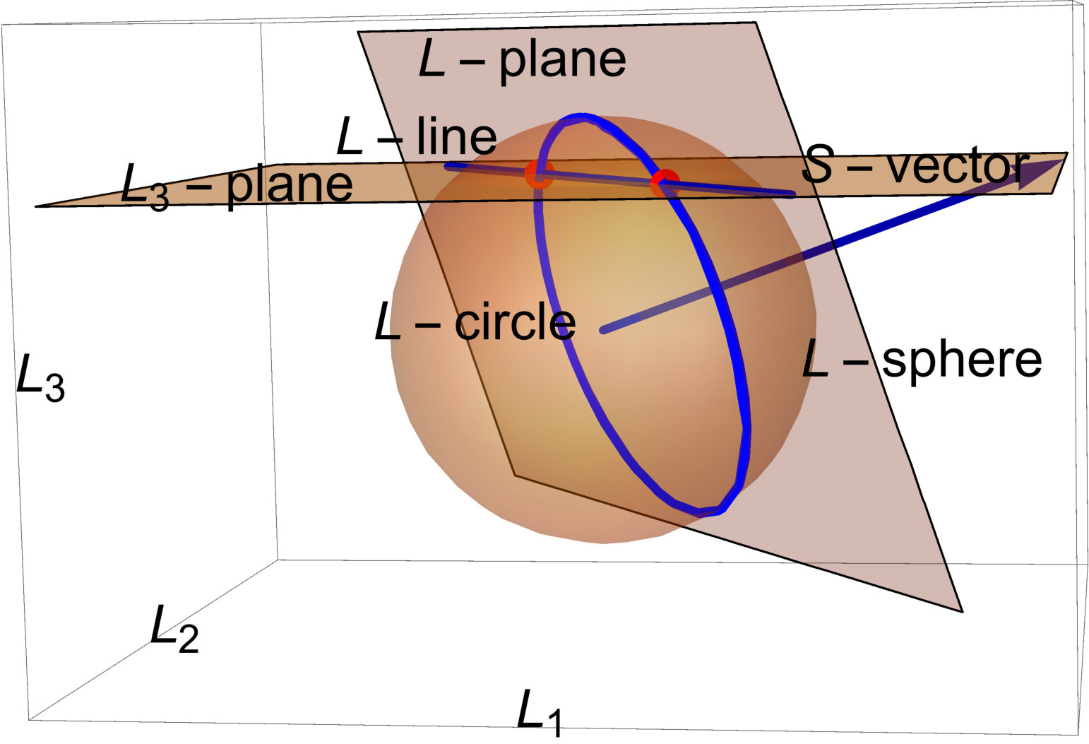 Figure 1
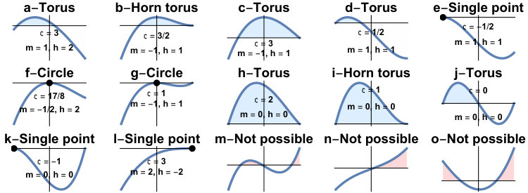 Figure 2
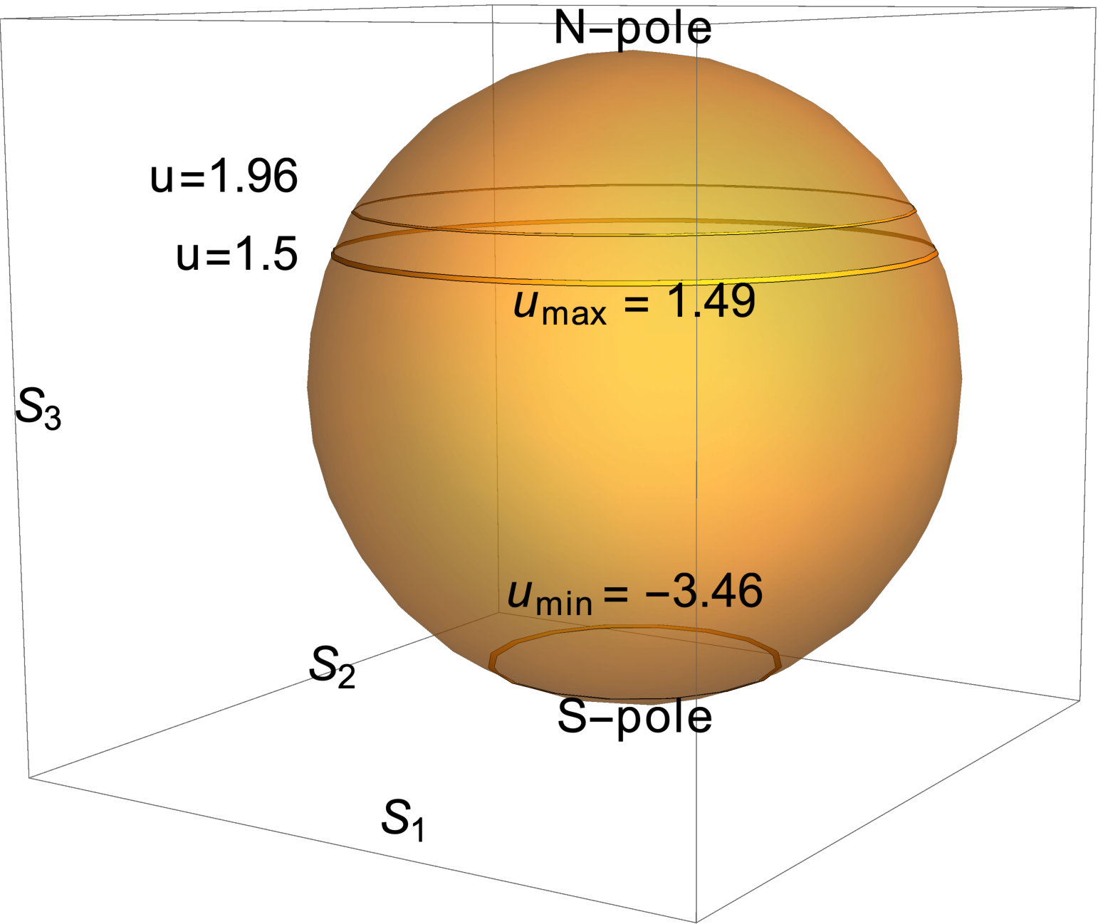 Figure 3
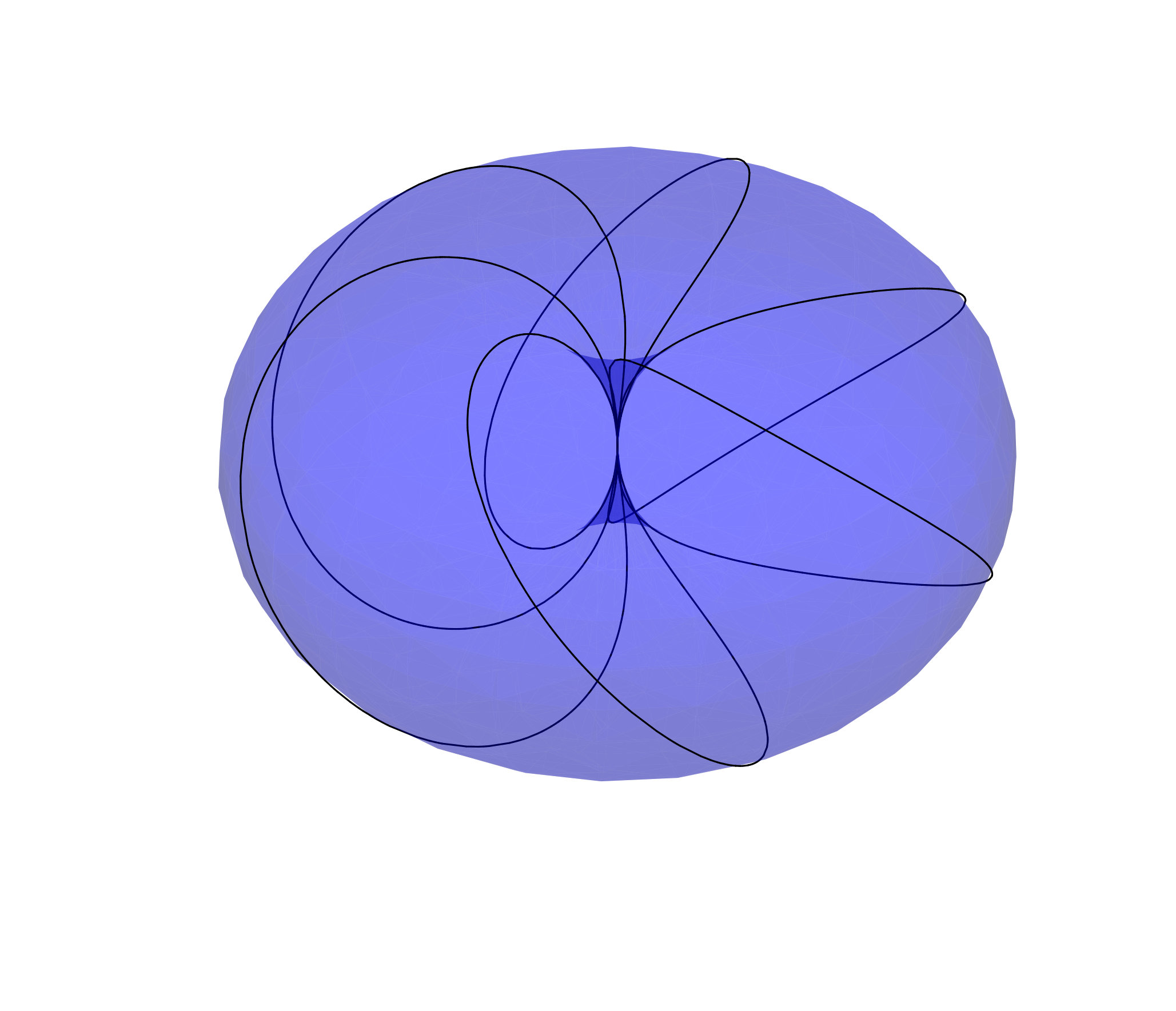 Figure 4
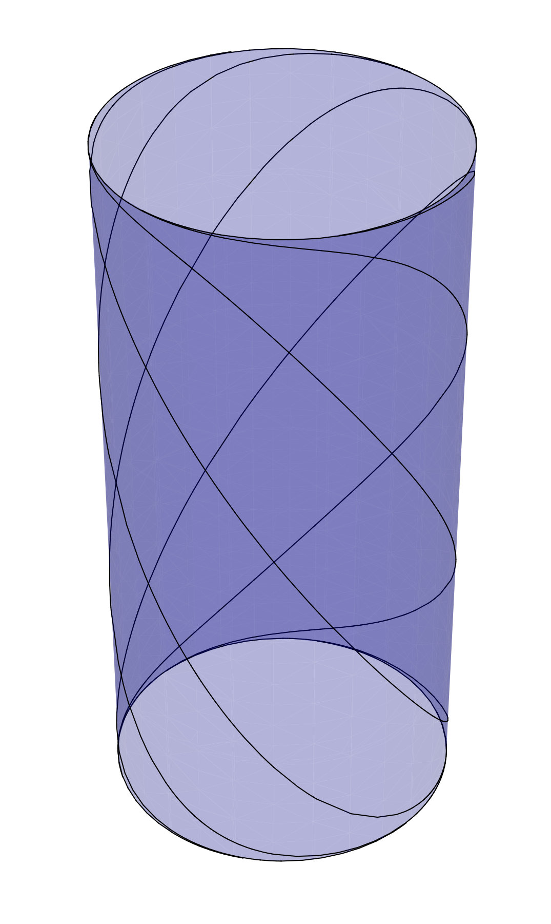 Figure 5
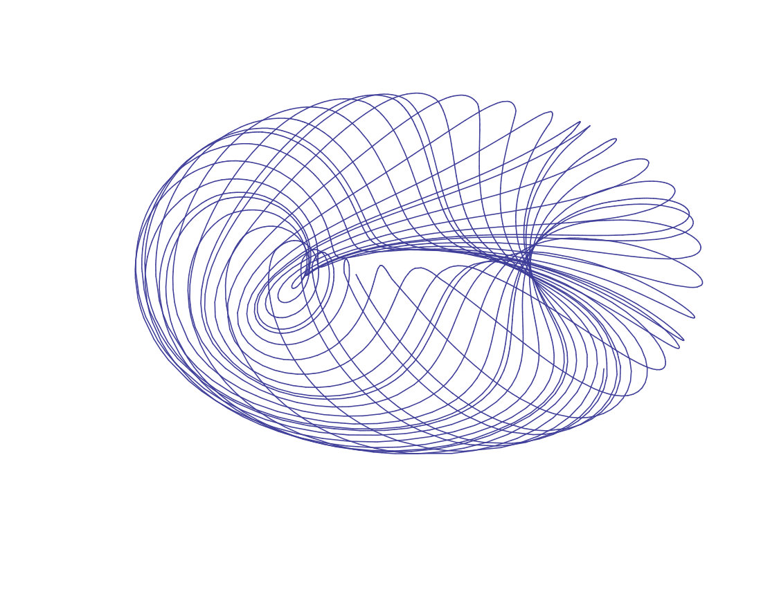 Figure 6
Peer Reviews
No public reviews on file for this paper yet. If you reviewed it on a platform where reviews are public (OpenReview, ICLR, NeurIPS, ICML), you can paste yours below so the community can read it here.
Videos
No videos yet. Explain this paper in a talk, walkthrough, or lecture? Add one.
arXiv:1906.03141[nlin.SI]
Invariant tori, action-angle variables and phase space structure of the Rajeev-Ranken model
Govind S. Krishnaswami and T. R. Vishnu
Physics Department, Chennai Mathematical Institute, SIPCOT IT Park, Siruseri 603103, India
Email: [email protected], [email protected]
(August 10, 2019
Published in J. Math. Phys. 60, 082902 (2019))
Abstract
We study the classical Rajeev-Ranken model, a Hamiltonian system with three degrees of freedom describing nonlinear continuous waves in a 1+1-dimensional nilpotent scalar field theory pseudodual to the SU(2) principal chiral model. While it loosely resembles the Neumann and Kirchhoff models, its equations may be viewed as the Euler equations for a centrally extended Euclidean algebra. The model has a Lax pair and -matrix leading to four generically independent conserved quantities in involution, two of which are Casimirs. Their level sets define four-dimensional symplectic leaves on which the system is Liouville integrable. On each of these leaves, the common level sets of the remaining conserved quantities are shown, in general, to be 2-tori. The non-generic level sets can only be horn tori, circles and points. They correspond to measure zero subsets where the conserved quantities develop relations and solutions degenerate from elliptic to hyperbolic, circular or constant functions. A geometric construction allows us to realize each common level set as a bundle with base determined by the roots of a cubic polynomial. A dynamics is defined on the union of each type of level set, with the corresponding phase manifolds expressed as bundles over spaces of conserved quantities. Interestingly, topological transitions in energy hypersurfaces are found to occur at energies corresponding to horn tori, which support purely homoclinic orbits. The dynamics on each horn torus is non-Hamiltonian, but expressed as a gradient flow. Finally, we discover a family of action-angle variables for the system that apply away from horn tori.
Keywords: Classical integrability, nonlinear waves, Euclidean algebra, nilpotent Lie algebra, Casimirs, symplectic leaves, common level sets, invariant tori, elliptic curve, gradient flow, action-angle variables.
Contents
-
3.1.1 Symplectic leaves and energy and helicity vector fields
-
3.2 Reduction to tori using conservation of energy and helicity
-
3.2.1 Reduction of canonical vector fields to and its topology
-
3.3 Classifying all common level sets of conserved quantities
-
3.3.3 Properties of and the closed, connectedness of common level sets
-
3.3.4 Possible types of common level sets of all four conserved quantities
-
3.4 Nature of the ‘Hill’ region and energy level sets using Morse theory
-
4 Foliation of phase space by tori, horn tori, circles and points
-
4.1 Union of circular level sets: Poisson structure & action-angle variables
-
4.2 Union of horn toroidal level sets: Dynamics as gradient flow
1 Introduction
The Rajeev-Ranken model [1, 2] is a Hamiltonian system with three degrees of freedom. It arises as a reduction of a -dimensional scalar field theory [3, 4] dual to the SU(2) principal chiral model (PCM) [5]. Unlike the PCM, which is asymptotically free, the dual scalar field is strongly coupled in the ultraviolet and could serve as a toy-model to study non-perturbative features of theories with a Landau pole. This scalar field theory also arises as a large-level, weak-coupling limit of the Wess-Zumino-Witten model [1]. In [1], the authors initiated the study of a class of highly nonlinear continuous waves in the scalar field theory, which could play a role similar to solitary waves in other field theories. The Rajeev-Ranken model is the reduction of the scalar field theory to the space of nonlinear screw-type waves of the form satisfying the field equations for the (2) Lie algebra-valued scalar field . Here, is a constant (2) matrix, a dimensionless parameter and a dimensionless coupling constant.
In [1], the evolution equations for in the Rajeev-Ranken model were formulated as the ODEs
[TABLE]
for a pair of three-dimensional vectors and related to and as in Eq. (4). These equations were shown to admit a Hamiltonian formulation based on a quadratic Hamiltonian and a step-2 nilpotent Lie algebra mimicking those of the scalar field theory, with solutions expressible in terms of elliptic functions. As we describe in Appendix A, the equations (1) may also be viewed as the Euler equations for a centrally extended Euclidean algebra and the quadratic Hamiltonian .
In [2], we studied the classical integrability of the Rajeev-Ranken model. We showed that it admits a family of degenerate but compatible Poisson structures, identified their Casimirs and found Lax pairs and -matrices for the model. The model was argued to be Liouville integrable by displaying a complete set of four generically independent conserved quantities in involution.
The Rajeev-Ranken model is related to two other interesting dynamical systems: (a) In [2], a formal relation between its equations and those of the Neumann model [6, 7] was obtained. Though not an equivalence (as the corresponding dynamical variables live in different spaces), it was exploited to find a new Hamiltonian formulation for the Neumann model. (b) Interestingly, Eqs. (1) also bear some resemblance to Kirchhoff’s equations for a rigid body moving in an ideal potential flow [8]. Roughly, and play the roles of total angular momentum and linear momentum of the body-fluid system in a body-fixed frame [9]. However, while the Poisson brackets of the Kirchhoff system are given by the Euclidean - Lie algebra, the Rajeev-Ranken model involves its central extension (see Appendix A).
The Rajeev-Ranken model may also be regarded as describing a special class of flat connections. Indeed, the currents and of the PCM (for the SU(2) group-valued principal chiral field ) are components of a flat (2) connection in 1+1-dimensions, satisfying the additional condition . Solutions of the dual scalar field theory thus furnish a special class of flat connections . There are other interesting integrable systems having to do with flat connections. For instance, in [10, 11, 12] the authors study integrable systems describing Hamiltonian dynamics on the space of flat connections on a Riemann surface. Evidently, while solutions to the Rajeev-Ranken model are very special classes of flat connections, the latter models deal with evolution on the space of all flat connections.
In this article, we continue our investigations into the structure of the phase space and classical integrability of the Rajeev-Ranken model. In [2], the question of finding all common level sets of conserved quantities and obtaining action-angle variables was posed. Here we find all common level sets and show that the phase space is foliated by four types of invariant tori [2-tori and their limits: horn tori (tori with equal major and minor radii - see Fig. 3), circles and points]. Moreover, we show that the union of common level sets of a given type may be treated as the phase space of a self-contained dynamical system. We construct action-angle variables for the dynamics on the union of 2-tori, which occupy all but a measure zero subset of the phase space. They degenerate to action-angle variables on the union of circular level sets. Interestingly, we find that the dynamics on the space of horn tori is not Hamiltonian, but expressible as a gradient flow. We now summarize the organization of the paper along with the principal results of each section.
In section 2, we introduce the Rajeev-Ranken model as a reduction of the 1+1-dimensional scalar field theory and discuss its Hamiltonian formulation and classical integrability.
In section 3, we use the conserved quantities and of the model to reduce the dynamics to their common level sets. To begin with, in section 3.1, assigning numerical values to the Casimirs and of the nilpotent Poisson algebra of section 2, enables us to reduce the six-dimensional degenerate Poisson manifold of the - variables () to its non-degenerate four-dimensional symplectic leaves . We also find Darboux coordinates on and use them to obtain a Lagrangian. Next, assigning numerical values to energy we find the generically three-dimensional energy level sets and use Morse theory to discuss the changes in their topology as the energy is varied (see section 3.4). Finally, in section 3.2 we consider the common level sets of all four conserved quantities and argue that they are generically diffeomorphic to 2-tori. This is established by showing that they admit a pair of commuting tangent vector fields (the canonical vector fields and associated to the conserved energy and helicity ) that are linearly independent away from certain singular submanifolds. Section 3.3 is devoted to a systematic identification of all common level sets of the conserved quantities and . We find that the condition for a common level set to be nonempty is the positivity of a cubic polynomial , which also appears in the nonlinear evolution equation for . Each common level set of conserved quantities may be viewed as a bundle over a band of latitudes of the -sphere , with fibres given by a pair of points that coalesce along the extremal latitudes (which must be zeros of ) (see Fig. 1). By analyzing the graph of the cubic (see Fig. 2) we show that the common level sets are compact and connected and can only be of four types: 2-tori (generic), horn tori, circles and single points (non-generic). The non-generic common level sets arise as limiting cases of 2-tori when the major and minor radii coincide, minor radius shrinks to zero or when both shrink to zero.
In section 4, we study the dynamics on each type of common level set. The union of single point common level sets comprises the static subset: it is the union of a two and a three-dimensional submanifold ( and ) of phase space. In section 4.1, we discuss the four-dimensional union of all circular level sets. Circular level sets arise when has a double zero at a non polar latitude of the -sphere. On , solutions reduce to trigonometric functions, the wedge product vanishes and the conserved quantities satisfy the relation , where is the discriminant of . Geometrically, may be realized as a circle bundle over a three-dimensional submanifold of the space of conserved quantities. Finally, we find a set of canonical variables on comprising the two Casimirs and and the action-angle pair and .
In section 4.2, we examine the four-dimensional union of horn toroidal level sets. It may be viewed as a horn torus bundle over a two-dimensional space of conserved quantities. Horn tori arise when the cubic is positive between a simple zero and a double zero at a pole of the -sphere. Solutions to the equations of motion degenerate to hyperbolic functions on and every trajectory is a homoclinic orbit which starts and ends at the center of a horn torus (see Fig. 3). As a consequence, the dynamics on is not Hamiltonian, though we are able to express it as a gradient flow, thus providing an example of a lower-dimensional gradient flow inside a Hamiltonian system. Interestingly, though the conserved quantities are functionally related on horn tori, the wedge product is non-zero away from their centers.
In section 4.3, we discuss the six-dimensional union of 2-toroidal level sets, which may be realized as a torus bundle over the subset of the space of conserved quantities. We use two patches of the local coordinates and to cover . The solutions of the equations of motion are expressed in terms of elliptic functions and the trajectories are generically quasi-periodic on the tori (see Fig 4). By inverting the Weierstrass- function solution for , we discover one angle variable. Next, by imposing canonical Poisson brackets, we arrive at a system of PDEs for the remaining action-angle variables, which remarkably reduce to ODEs. The latter are reduced to quadrature allowing us to arrive at a fairly explicit formula for a family of action-angle variables. In an appropriate limit, these action-angle variables are shown to degenerate to those on the circular submanifold .
It is satisfying that a detailed and explicit analysis of the dynamics and phase space structure of this model has been possible using fairly elementary methods. Our results should be helpful in understanding other aspects of the model’s integrability (bi-Hamiltonian formulation on symplectic leaves, spectral curve etc.), the stability of its solutions, effects of perturbations and its quantization (for instance via our action-angle variables, through the representation theory of nilpotent Lie algebras or via path integrals using our Lagrangian obtained from Darboux coordinates, to supplement the Schrödinger picture results in [1]). Quite apart from its physical origins and possible applications, we believe that the elegance of the Rajeev-Ranken model justifies a detailed study. It is hoped that the insights gained can then also be usefully applied to understanding the parent scalar field theory.
2 Formulation of the classical Rajeev-Ranken model
The scalar field theory whose reduction leads to the Rajeev-Ranken model [1] was introduced by Zakharov and Mikhaliov [3] and Nappi [4]. It is defined by the nonlinear field equations
[TABLE]
Here, the traceless anti-hermitian matrix is an Lie algebra-valued scalar field. Using the screw-type (internal rotation and translation) continuous wave ansatz:
[TABLE]
Eq. (2) reduces to a system of ODEs for a mechanical system with three degrees of freedom. Here and the wave number are real parameters. Unlike solitons, these nonlinear waves have constant energy density [1]. Introducing the matrices
[TABLE]
which play the roles of and , the equations of motion (2) become six first order equations
[TABLE]
for the components and , where are the Pauli matrices. Here, is non-dynamical. We will often use polar coordinates () for
[TABLE]
and work with the dimensionless variable in place of . The equations of motion (5) of the Rajeev-Ranken model follow from the Hamiltonian
[TABLE]
in conjunction with the step-2 nilpotent Poisson algebra
[TABLE]
for . Interestingly, (5) also follow from the same Hamiltonian and the distinct but compatible non-nilpotent Euclidean Poisson algebra
[TABLE]
Both the nilpotent and Euclidean algebras are degenerate. Their centers are generated by the Casimirs and respectively, where
[TABLE]
In fact, there is a degenerate Poisson pencil’s worth of brackets (see §4.2 of [2])
[TABLE]
all of which imply (5) with the same Hamiltonian (7). Henceforth, we work with the nilpotent Poisson structure so that and are non-Casimir conserved quantities. The Hamiltonian (7) can be expressed as
[TABLE]
The equations of motion (5) were shown [2] to be equivalent to the Lax equation with spectral parameter where
[TABLE]
The conserved quantities and arise as coefficients of powers of in . They are in involution due to the existence of an -matrix:
[TABLE]
Here, is the permutation matrix. In [2], it was shown that and are a complete and generically independent set of conserved quantities. Along with their involutive property, this was used to argue that the dynamics on each four-dimensional symplectic leaf (obtained by fixing the values of the two Casimirs and ) must be Liouville integrable.
3 Using conserved quantities to reduce the dynamics
In this section, we discuss the reduction of the six-dimensional - phase space () by successively assigning numerical values to the conserved quantities and . For each value of the Casimirs and we obtain a four-dimensional manifold with non-degenerate Poisson structure, which is expressed in local coordinates along with the equations of motion. Next, we identify the (generically three-dimensional) constant energy submanifolds , where is a function of and (12). Moreover, we use Morse theory to study the changes in topology of with changing energy. Finally, the conservation of helicity allows us to reduce the dynamics to generically two-dimensional manifolds , which are the common level sets of all four conserved quantities. By analysing the nature of the canonical vector fields and , the latter are shown to be 2-tori in general. We also argue that there cannot be any additional independent integrals of motion. Though the common level sets of all four conserved quantities are generically 2-tori, there are other possibilities. We show that has the structure of a bundle over a portion of the sphere , determined by the zeros of a cubic polynomial . By analyzing the possible graphs of we show that is compact, connected and of four possible types: tori, horn tori, circles and points.
3.1 Using Casimirs and to reduce to 4D phase space
3.1.1 Symplectic leaves and energy and helicity vector fields
The common level sets of the Casimirs and are the four-dimensional symplectic leaves of the phase space . On , the Poisson tensor corresponding to the nilpotent Poisson algebra (8) (see also §4.1 of [2]) is non-degenerate and may be inverted to obtain the symplectic form . In Cartesian coordinates ,
[TABLE]
This symplectic form is the exterior derivative of the canonical 1-form . Expressing helicity (10) and (12) as functions on by eliminating
[TABLE]
we obtain the helicity and Hamiltonian vector fields on (see also Eq. (61) of [2])
[TABLE]
Since and commute, . It is notable that is non-zero except at the origin (), while vanishes at the origin and on the circle (). The points where and vanish turn out be the intersection of with the static submanifolds
[TABLE]
introduced in §5.5 of [2], where and are time-independent. The points where vanish will be seen in §3.4 to be critical points of the energy function.
3.1.2 Darboux coordinates on symplectic leaves
Since it is natural to look for global canonical coordinates. In fact, the canonical coordinates on the six-dimensional phase space (which were introduced in §4.3 of [2]) restrict to Darboux coordinates on :
[TABLE]
with and . The Hamiltonian is a quartic function in these coordinates:
[TABLE]
The equations of motion resulting from these canonical Poisson brackets and Hamiltonian are cubically nonlinear ODEs. In fact, for :
[TABLE]
A Lagrangian , leading to these equations of motion can be obtained by extremizing with respect to and :
[TABLE]
3.2 Reduction to tori using conservation of energy and helicity
So far, we have chosen (arbitrary) real values for the Casimirs and to arrive at the reduced phase space . Now assigning numerical values to the Hamiltonian we arrive at the generically three-dimensional constant energy submanifolds which foliate . It follows from the formula for the Hamiltonian (12) that each of the is bounded above in magnitude by . Moreover, is closed as it is the inverse image of a point. Thus, constant energy manifolds are compact. Interestingly, the topology of can change with energy: this will be discussed in §3.4. In addition to the Hamiltonian and Casimirs and , the helicity is a fourth (generically independent) conserved quantity (see §5.7 of [2]). Thus each trajectory must lie on one of the level surfaces of that foliate . Note that since is uniquely determined by (and vice versa), the level sets of the conserved quantities and are in 1-1 correspondence and we will use the two designations interchangeably.
We will see in §3.2.1 that these common level sets of conserved quantities are generically 2-tori, parameterized by the angles and which (as shown in §5.2 of [2]) evolve according to
[TABLE]
Here, is related to and via helicity and (10)
[TABLE]
In other words, the components and of the Hamiltonian vector field are functions of alone. Though the denominators in (25) could vanish, the quotients exist as limits, so that is non-singular on . Interestingly, as pointed out in [1], evolves by itself as we deduce from (5):
[TABLE]
This cubic will be seen to play a central role in classifying the invariant tori in §3.3. The substitution , reduces this ODE to Weierstrass normal form
[TABLE]
with solution . Here, the Weierstrass invariants are (there is a minor error in in [1])
[TABLE]
Thus we obtain
[TABLE]
which oscillates periodically in time between and , which are neighbouring zeros of between which is positive. Choosing fixes the initial condition, with its real part fixing the origin of time. In particular, if (the imaginary half-period of ), then . On the other hand, if , where is the real half-period. The formula (30) will be used in §4.3 to find a set of action-angle variables for the system.
3.2.1 Reduction of canonical vector fields to and its topology
In this section, we use the coordinates to show that the canonical vector fields and are tangent to the level sets , which are shown to be compact connected Lagrangian submanifolds of the symplectic leaves . Moreover, and are shown to be generically linearly independent and to commute, so that are generically 2-tori.
On , the coordinates (as opposed to ) are convenient since the common level sets arise as intersections of the and coordinate hyperplanes. The remaining variables and furnish coordinates on . The Poisson tensor on in these coordinates has a block structure, as does the symplectic form:
[TABLE]
where and are the dimensionless matrices:
[TABLE]
Here and and are as in (25), subject to the relation (26). From (10), it follows that and may be expressed in terms of and , by solving the pair of equations
[TABLE]
Here . In these coordinates, and (18) have no components along or :
[TABLE]
Thus, and are tangent to . Moreover, the restriction of to is seen to be identically zero as it is given by the - block in (31) so that is a Lagrangian submanifold. Trajectories on are the integral curves of .
To identify the topology of the common level set , it is useful to investigate the linear independence (over the space of functions) of the vector fields and . On , is non-degenerate so that and are linearly independent iff . We find that this wedge product vanishes on precisely when and satisfy the relations
[TABLE]
Here etc., and and are expressed using (16). It was shown in §5.6 of [2] that (36) are the necessary and sufficient conditions for the four-fold wedge product to vanish in . Moreover, it was shown that this happens precisely on the singular set which consists of the circular/trigonometric submanifold and its boundaries and . Thus, and are linearly independent away from the set (of measure zero) given by the intersection of with . [For given and , the intersection of with is in general a two-dimensional manifold defined by four conditions among the six variables and : and (with ) as well as the conditions in Eq. (16).] Furthermore, since and Poisson commute, . So, as long as we stay away from these singular submanifolds, and are a pair of commuting linearly independent vector fields tangent to (see Lemma 1 in Chapter 10 of [13]). Additionally, we showed at the beginning of §3.2 that the energy level sets are compact manifolds. Now, must also be compact as it is a closed subset of (the inverse image of a point). Finally, we will show in §3.3.4 that is connected. Thus, for generic values of the conserved quantities, is a compact, connected surface with a pair of linearly independent tangent vector fields. By Lemma 2 in Chapter 10 of [13], it follows that the common level sets of conserved quantities are generically diffeomorphic to -tori.
We observed in §5.2 of [2] that a generic trajectory on a 2-torus common level set is dense (see also Fig. 4). This implies that any additional continuous conserved quantity would have to be constant everywhere on the torus and cannot be independent of the known ones. Thus, we may rule out additional independent conserved quantities.
3.3 Classifying all common level sets of conserved quantities
In §3.2 we showed that the common level sets of the conserved quantities and are generically 2-tori. However, this leaves out some singular level sets. These non-generic common level sets occur when the conserved quantities fail to be independent and also correspond to the degeneration of the elliptic function solutions (30) to hyperbolic and circular functions. Here, we use a geometro-algebraic approach to classify all common level sets and show that there are only four possibilities: 2-tori, horn tori, circles and single points. Interestingly, the analysis relies on the properties of the cubic that arose in the equation of motion for (27).
3.3.1 Common level sets as bundles and the cubic
We wish to identify the submanifolds of phase space obtained by successively assigning numerical values to the four conserved quantities and . Not all real values of these conserved quantities lead to non-empty common level sets. From (7), we certainly need the Hamiltonian and . It follows that . However, these conditions are not always sufficient; additional conditions will be identified below. The situation is analogous to requiring the energy ( in the principle axis frame) and square of angular momentum to be non negative for force-free motion of a rigid body. These two conditions are necessary but not sufficient to ensure that the angular momentum sphere and inertia ellipsoid intersect.
First, putting defines a -sphere (the -sphere’) in the -space as in Fig. 1(a). We may regard (or ) for as the latitude on the -sphere with representing the North and South poles. At each point on the -sphere, the conservation of helicity forces to lie on a plane (the -plane’) perpendicular to the numerical vector at a distance from the origin of the -space. At this point, we have assigned numerical values to and , which happen to be Casimirs of the Euclidean Poisson algebra (9). It remains to impose the conservation of and .
For each point on the -sphere, the condition (10) defines an -sphere of radius in the -space provided . Since , the conserved quantities must be chosen to satisfy . In fact, this ensures that and thus subsumes the latter. The -sphere and the -plane intersect along an -circle provided the radius of the -sphere exceeds the distance of the -plane from the origin, i.e.,
[TABLE]
Thus, for the intersection to be non-empty, depending on the sign of , must lie below or above a particular latitude determined by (37). Furthermore, since , we must choose
[TABLE]
When the inequality (37) is saturated, the -plane is tangent to the -sphere and the -circle shrinks to a point. In summary, the common level set of the three conserved quantities and can be viewed as a sort of fibre bundle with base given by the portion of the -sphere lying above or below a given latitude. The fibres are given by -circles of varying radii which shrink to a point along the extremal latitude.
The final conserved quantity restricts to the horizontal plane . For each non-polar point on the -sphere, this -plane intersects the above -plane along the -line (assuming are not both zero). This line intersects the -sphere at a pair of points, provided the radius of the -sphere is greater than the distance of the -line from the origin of the -space, i.e.
[TABLE]
The two points of intersection coincide if the inequality is saturated so that the -line is tangent to the -sphere. Note that inequality (39) implies (37), provided the -sphere is non-empty (). This is geometrically evident since the distance of the -line from the origin is bounded below by the distance of the -plane (which contains the -line) from the origin.
Remark: Another way to see that (39) implies (37) is to note that if , then
[TABLE]
Eq. (39) would then imply (37), if we can show that on the sphere . To see this, we first note that at the poles so that it suffices to show that the quadratic polynomial is non-negative for . This is indeed the case since the global minimum of attained at is simply zero.
Assuming (39) holds, the common level set of all four conserved quantities may be viewed as a sort of fibre bundle with base given by the part of the -sphere satisfying (39) and fibres given by either one or a pair of points (this is the case for non-polar latitudes, see below for the special circumstance that occurs above the poles). In other words, provided , the ‘base’ space is the part of the -sphere consisting of all latitudes lying in the interval and satisfying the cubic inequality following from (39)
[TABLE]
The roots of the cubic equation resulting from the saturation of this inequality determine the extremal latitudes where the two-point fibres degenerate to a single point (provided the extremal latitude does not correspond to a pole of the -sphere). If an extremal latitude is at one of the poles then must vanish there and the determination of the fibre over the pole is treated below.
Recall that the discriminant of the cubic is the product of squares of differences between its roots. It vanishes iff a pair of roots coincide. The discriminant of the cubic will be useful in the analysis that follows. It is a function of the four conserved quantities:
[TABLE]
3.3.2 Fibres over the poles of the -sphere
At the and poles of the -sphere, the -plane and -plane are both horizontal: their intersection does not define an -line. For the common level sets of and to be non-empty, the planes must coincide:
[TABLE]
with upper/lower signs corresponding to the poles. This condition ensures that vanishes at the corresponding pole, implying that it cannot be positive at a physically allowed pole of the -sphere.
Now, for the -sphere to intersect the -plane, its radius must be bounded below by :
[TABLE]
When this inequality is strict, the fibre over the pole is a circle (-circle) while it is a single point when the inequality is saturated. Interestingly, in the latter case, the discriminant (43) vanishes, so that the pole must either be a double or triple zero of . On the other hand, when the inequality is strict, must have a simple zero at the pole. This structure of fibres over the poles is in contrast to the two point fibres over the non polar latitudes of the -sphere when . For example, suppose and take so that the and -planes over the pole coincide. These planes intersect the -sphere provided (see (45)). Moreover, the fibre over the pole is a single point if and a circle if .
3.3.3 Properties of and the closed, connectedness of common level sets
We observed in §3.3.2 that must vanish at a physically allowed pole of the -sphere and that we must have for this to happen. Here, we investigate the possible behaviour of near a pole, which helps in restricting the allowed graphs of . We find that the sign of at an allowed pole is fixed and also that the allowed latitudes must form a closed and connected set. As a consequence, we deduce that some graphs of are disallowed. For example, cannot have a triple zero at a non-polar latitude. We also deduce that the common level sets must be both closed and connected.
Result 1: Sign of at a pole which is a simple zero: Suppose has a simple zero at the pole with non-empty fibre over it, then .
Proof of : Suppose , so that has a simple zero at the pole with circular fibre over it (see Eq.(44)). Then (41) implies
[TABLE]
Suppose , then . But in this case, the upper bound on the latitude so that could not have been an allowed latitude. On the other hand, if , then is an allowed latitude. Thus, when the pole for is a simple zero of with non-empty fibre, it is always surrounded by other allowed latitudes. In particular, the north poles in Fig. 2g, j and k are not allowed latitudes, while they are in Fig. 2c and h.
Proof of : On the other hand, suppose so that has a simple zero at with non-empty fibre. Suppose , then as before (41) implies which violates (38). Thus must be positive. In other words, when the pole is a simple zero of with non-empty fibre, it must be surrounded by other allowed latitudes. So the poles cannot be simple zeros unless the neighbouring latitudes are allowed. In particular, the south poles in Fig. 2d, h, i and j are allowed latitudes.
Result 2: Set of allowed latitudes and common level set must be closed: The conserved quantities and define continuous functions (quadratic in and ) from the phase space to the four-dimensional space of conserved quantities (which is a subset of consisting of the 4-tuples subject to the conditions and (38)). Each of their common level sets must be a closed subset of as it is the inverse image of a point in . We may use this to deduce that cannot approach a positive value at a pole. We have already observed that if a pole is an allowed latitude then must vanish there. On the other hand, suppose a pole is not an allowed latitude but is positive in a neighbourhood of . Then the set of allowed latitudes would be an open set and so would the common level set. In particular, cannot have (i) only one simple zero on the -sphere and be non-vanishing elsewhere (as in Fig. 2n) (ii) three simple zeros between the poles (see Fig. 2m) (iii) a double zero and a simple zero between the poles (iv) a triple zero at a non-polar latitude (v) two simple zeros between the poles with at the poles (as in Fig. 2o) or (vi) a double zero between the poles with at the poles.
Common level set of conserved quantities must be connected: For the common level set to be disconnected, the set of allowed latitudes on the -sphere must be disconnected. The only remaining way that this could happen is for to have three distinct simple zeros on latitudes of the -sphere. Let us show that this is disallowed. Now Result 2 prevents from having three simple zeros at non-polar latitudes. It only remains to consider the cases where either of the poles is a simple zero of . If has a simple zero at , then by Result 1, . Since , can have at most one more zero on the -sphere so that the set of allowed latitudes is connected. On the other hand, suppose has a simple zero at , then by Result 1. Suppose further that has two more simple zeros on the -sphere, then by Result 2, must equal as otherwise would be positive at the pole as in the disallowed Figs. 2m, n and o. So with as in Fig. 2j. But in this case, Result 1 forbids from being an allowed latitude, so that the set of allowed latitudes is again a single interval .
Triple zeros of : For (41) to have a triple zero, i.e., to be of the form , we must have and the conserved quantities must satisfy two conditions:
[TABLE]
These conditions define a two-dimensional surface in the space of conserved quantities. Result 2 implies that cannot have a triple zero at a non-polar latitude. On the other hand, can have a triple zero at or provided both (44) and (47) are satisfied. Putting in (47), the conditions for or to be a triple zero become
[TABLE]
The first condition implies that cannot have a triple zero at for or at for . On the other hand, can have a triple zero at for as in Fig. 2l.
3.3.4 Possible types of common level sets of all four conserved quantities
Here we combine the above results on the connectedness of common level sets, slope of at the poles and on the structure of the fibres over polar and non-polar latitudes of the -sphere to identify all possible common level sets of conserved quantities. There are only four possibilities: the degenerate or singular level sets (horn tori, circles and single points) and the generic common level sets (2-tori). These possibilities are distinguished by the location of roots of . They are discussed below and illustrated in Fig 2. In (C1)-(C5) below we take so that correspond to the and poles. Similar results hold for with and interchanged.
(C1) For generic values of conserved quantities, is positive between two neighbouring non-polar simple zeros lying in (E.g. , and as in Fig. 2a). The base space of §3.3 is the portion of the -sphere lying between the latitudes and , with the two-point fibres shrinking to single point fibres along the extremal latitudes and . The resulting common level set is homeomorphic to a pair of finite coaxial cylinders with top as well as bottom edges identified, i.e., a -torus.
To visualize the above toroidal common level sets and some of its limiting cases which follow, it helps to qualitatively relate the separation between zeros of to the geometric parameters of the torus embedded in three dimensions. For instance, the minor diameter of the torus grows with the distance between and . Thus, when the simple zeros coalesce at a double zero, the minor diameter vanishes and the torus shrinks to a circle. Similarly (for ) the major diameter of the torus grows with the distance between and . Thus, when , the major and minor diameters become equal and we expect the torus to become a horn torus. However, this requires the fibre over to be a single point, which is true only when is a double zero of .
(C2) A limit of (C1) where either or and is positive between them. For instance, if and the fibre over is a single point, then the common level set is homeomorphic to a horn torus (E.g. , and as in Fig. 2b). On the other hand, for the fibre over is a circle and we expect the common level set to be a -torus (see Fig. 2c). It is as if the circular fibre over the single-point latitude plays the role of an extremal circular latitude with single point fibre in (C1), thus the roles of base and fibre are reversed. Similarly, when with circular fibre over , the common level set is homeomorphic to a 2-torus (E.g. and as in Fig. 2d). In the limiting case where , the two simple zeros and merge at . The fibre over becomes a single point and the common level shrinks to a point (see Fig. 2e).
(C3) Another limit of (C1) where the roots and coalesce at a double root of . is negative on the -sphere except along the latitude and the fibre over it is a single point. The discriminant (43) must vanish for this to happen. The common level set becomes a circle corresponding to the latitude . For example, if and and , then the equator is the allowed latitude as shown in Fig. 2f. Another example of a circular common level set appears in Fig. 2g. In this case Results 1 and 2 exclude the north pole ensuring the connectedness of the common level set.
(C4) A limit of (C1) where the simple zeros and move to and respectively, with in between. In this case, both poles have circular fibres and the common level set is a 2-torus. This happens, for instance, when , irrespective of the values of and . Another way for this to happen is for and to vanish so that the poles are automatically zeros of
[TABLE]
and to choose to ensure there is no zero in between. Holding and fixed, three more possibilities arise as we decrease . When , has a double zero at (Fig. 2i) with a single point fibre over it and the common level set becomes a horn torus. For , the third zero of moves from to the latitude . By Result 1, the allowed latitudes go from to (see Fig. 2j), and the common level set returns to being a -torus. Finally, when , the only allowed latitude is a double zero and the common level set shrinks to a point (see Fig. 2k).
(C5) has a zero at just one of the poles and is negative elsewhere on the -sphere. The common level set is then a single point. We encountered this as a limiting case of (C2) where has a double zero at as in Fig. 2e. This can also happen when is negative on the -sphere except for a triple zero at either () or () (see Eq. (48)). For example, when , and , has a triple zero at as in Fig. 2l.
3.4 Nature of the ‘Hill’ region and energy level sets using Morse theory
In this section, we study the ‘Hill’ region , which we define as the set of points on the symplectic leaf with energy less than or equal to :
[TABLE]
The energy level set is then the boundary of . Taking and (20) as coordinates on , we treat the Hamiltonian
[TABLE]
as a Morse function [14]. The nature of critical points of depends on the value of . There are two types of critical points: (a) an isolated critical point at which exists for all values of and (b) a ring of critical points
[TABLE]
which exists only for and shrinks to the isolated critical point when . The energy at these critical points is
[TABLE]
Upon varying and , the isolated critical points cover all of the static submanifold while the rings of critical points cover the static submanifold . By finding the eigenvalues of the Hessian of the Hamiltonian at these critical points, we find that for the isolated critical point G is a local minimum of energy (four +ve eigenvalues). In fact, for , the isolated critical point has to be the global minimum of energy as the energy is bounded below and there are no other extrema of energy. For , the isolated critical point becomes a saddle point (two +ve and two -ve eigenvalues) with energy . On the other hand, the ring of critical points are degenerate global minima (three +ve and one zero eigenvalue). To apply Morse theory, we need the indices of the critical points of (number of negative eigenvalues of the Hessian). From the foregoing, we see that the ground state G has index zero, the saddle point has index two and the degenerate critical points on the ring may be nominally assigned a vanishing index.
Change in topology of the Hill region: According to Morse theory [14], the topology of the Hill region can change only at critical points of the Hamiltonian. (a) For , there is only one critical point, the global minimum G with index zero and energy . Thus, as increases beyond , the Hill region goes from being empty to being homeomorphic to a 4-ball arising from the addition of a 0-cell. (b) For , there are two critical values of energy corresponding to the ring of critical points and the saddle point. The index vanishes along the ring of critical points, so when crosses , the Hill region acquires a 3-ball (0-cell) for each point on the ring corresponding to the 3 positive eigenvalues of the Hessian. Thus for . The saddle point with has index two, so the topology of changes to upon adding a 2-cell to (the analogous statement in one lower dimension is that adding a 2-cell to the hole of the solid torus gives a ).
Nature of energy level sets: The energy level set is the boundary of the Hill region, i.e. . It is a 3-manifold except possibly at the critical energies. Thus for , for all energies . On the other hand, when the energy level set undergoes a change in topology from to as crosses .
The energy level sets at the critical values and are exceptional. For given and with and , is a single point on (the critical point), since G is the non-degenerate global minimum of energy. When , fixes leaving a range of possible values of , whose values are determined by eliminating from the conditions . This leads to a three-dimensional energy level set. includes one horn torus with its center as the saddle point for as well as a one parameter family of toroidal level sets for and a pair of circular level sets occurring at and . Interestingly, horn tori arise only when , since is a necessary condition for horn tori (see §4.2). Thus, the horn torus is a bit like the figure-8 shaped separatrix one encounters in particle motion in a double well potential. Finally, the level manifold consists of a ring of single point common level sets, each lying on the static submanifold . Unlike static solutions and horn tori, circular and 2-toroidal level sets also arise at non-critical energies.
4 Foliation of phase space by tori, horn tori, circles and points
For generic allowed values of the conserved quantities and , their common level set in the phase space is a -torus. As noted, this happens when has simple zeros along a pair of latitudes of the -sphere and is positive between them. However, this -parameter family of invariant tori does not completely foliate the phase space: there are some other ‘singular’ level sets as well: horn tori, circles and points. The union of single-point level sets is (19), consisting of static solutions. They occur when has a triple zero at or is a local maximum at a double zero at . We will now discuss the other cases in increasing order of complexity. In each case, we view the union of common level sets of a given type as the state space of a self-contained dynamical system which has the structure of a fibre bundle over an appropriate submanifold of the space of conserved quantities. The fibres in each case are circles, horn tori and tori. The dynamics on the union of circles and tori is Hamiltonian and we identify action-angle variables on them. On the other hand, we show that the dynamics on the union of horn tori is a gradient flow.
4.1 Union of circular level sets: Poisson structure & action-angle variables
In this section, we show that the union of circular level sets is the same as the trigonometric/circular submanifold (introduced in §5.6 of [2]) where the solutions are sinusoidal functions of time. Local coordinates on are furnished by and (or equivalently ) and we express the Hamiltonian in terms of them. The Poisson structure on is degenerate with and generating the center and their common level sets being the symplectic leaves. While is a constant of motion, evolves linearly in time. We exploit these features to obtain a set of action-angle variables for the dynamics on .
4.1.1 as a circle bundle and dynamics on it
As pointed out in example (C3) of §3.3.4, the common level set of conserved quantities is a circle when the cubic (41) has a double zero at a non-polar latitude of the -sphere and is negative on either side of it. In this case, the latitude is restricted to the location of the double zero. To identify the three-dimensional hypersurface in the four-dimensional space of conserved quantities, where has a double zero at a non-polar latitude, we will proceed in two steps. First, we compare the equation with to arrive at the three conditions:
[TABLE]
The first two may be used to express the roots and in terms of conserved quantities:
[TABLE]
The third equation in (54) then leads to the following conditions among conserved quantities
[TABLE]
Squaring, these conditions are equivalent to , where is the discriminant (43) of . The three-dimensional submanifold of defined by , however, includes 4-tuples (, , , ) corresponding to horn toroidal (double zero at the pole ) or single-point (triple zero at or double zero at or ) common level sets, in addition to circular level sets. To eliminate the former, we must impose the further conditions , and . This last condition, which says , selects the roots in (55). These conditions define the three-dimensional hypersurface corresponding to circular level sets. Now, and may be chosen as coordinates on , with (56) allowing us to express in terms of them. Interestingly, we find by studying examples, that for values of and corresponding to a circular level set, there are generically two distinct values of ; so we would need two such coordinate patches to cover . The union of all these circular level sets may be viewed as a sort of circle bundle over and forms a four-dimensional ‘circular’ submanifold of . As shown in §5.5 and §5.6 of [2], this circular submanifold along with its boundary coincides with the set where the four-fold wedge product vanishes.
The equations of motion (5) simplify on the circular submanifold . Indeed, since is a constant, so that implying that where . As shown in §5.5 of [2], the equations of motion then simplify to
[TABLE]
with sinusoidal solutions:
[TABLE]
Here, using (6), , which varies with location on the base . It is the non-dimensional angular velocity for motion in the circular fibres. Since and are positive, . Here both and evolve linearly in time and the equality of
[TABLE]
implies that the constant of motion may be expressed in terms of and :
[TABLE]
Remark: If the -sphere shrinks to a point then one still has circular level sets consisting of latitudes of the -sphere determined by , provided . However, each point on these exceptional circular level sets is a static solution lying on (19).
4.1.2 Canonical coordinates on
Local coordinates on : For the analysis that follows, a convenient set of coordinates on the ‘circle bundle’ consists of and for the base and for the fibres. The dynamics on admits three independent conserved quantities as there is one relation among and following from (56). Since the common level sets of the conserved quantities on are circles, rather than tori, it is reasonable to expect there to be two Casimirs (say and ) for the Poisson structure on , as we show below. In fact, is foliated by the common level surfaces of and (symplectic leaves) which serve as phase spaces (with coordinates and ) for a system with one degree of freedom. is then the coordinate along the circular level sets of the Hamiltonian on these two-dimensional symplectic leaves.
To find the reduced Hamiltonian on we express the remaining variables in terms of and . The formula for (10) along with (60) determines and consequently as well. The remaining conserved quantities are given by
[TABLE]
Thus, the reduction of the Hamiltonian (7) to the trigonometric submanifold is
[TABLE]
As remarked, for given values of and , there are generically two possible values of corresponding to two points on . By considering examples, we verified that for each of them, there is a unique that satisfies (60) and both the equations in (62).
Poisson structure on : We wish to identify Poisson brackets among the coordinates and that along with the reduced Hamiltonian (63) gives the equation of motion on . As noted, it is natural to take and as Casimirs so that . The only non-trivial Poisson bracket is then determined as follows from (63):
[TABLE]
Moreover, this implies , which notably differs from the original nilpotent Poisson bracket (8).
Canonical action-angle variables on : Since evolves linearly in time, it is a natural candidate for an angle variable. The corresponding canonically conjugate action variable must be a function of and and is determined from (64) by the condition . We thus obtain, up to an additive constant, the action variable
[TABLE]
Thus we arrive at the remarkably simple conclusion that (aside from the Casimirs and ) and are action-angle variables on . Moreover, the canonical Poisson bracket agrees with that on the full phase space (see (87)). Our reason to work with rather than as a coordinate is that the solutions (58) and the Hamiltonian (63) have simple expressions in terms of . By solving the cubic (65), can be expressed in terms of , which would allow us to write the Hamiltonian in terms of the action variable .
4.2 Union of horn toroidal level sets: Dynamics as gradient flow
Just as with the union of circular level sets , the union of horn toroidal level sets serves as the phase space for a self-contained dynamical system. However, unlike the sinusoidal periodic trajectories on , all solutions on are hyperbolic functions of time and are in fact homoclinic orbits joining the center of a horn torus to itself (see Fig. 3). The centers themselves are static solutions. Horn tori arise only when the energy is equal to the critical value given in §3.4. Thus, the horn tori are like the figure-8 shaped separatrices in the problem of a particle in a double well potential, separating two families of 2-tori. Interestingly, though the conserved quantities satisfy a relation on each horn torus, the four-fold wedge product vanishes only at its center. Finally, unlike on the circular submanifold, the flow on the horn-toroidal submanifold is not Hamiltonian, though we are able express it as a gradient flow.
The family of horn toroidal level sets is a two-dimensional submanifold of the four-dimensional space of conserved quantities . To see this, note that a horn torus arises when the cubic of (41) is positive between a simple zero and a double zero at the pole of the -sphere. Thus, must be of the form where with . These requirements imply and . Note that each non-trivial horn torus is a smooth two-dimensional surface except at its center which lies at the pole . Trivial horn tori are those that have shrunk to the points at their centers and arise when . The conditions and lead to two relations among conserved quantities
[TABLE]
which together imply that . The inequality along with (66) restricts us to points above a parabola in the - plane:
[TABLE]
The space is given by the set of such pairs. For each we get a horn torus . The union of all horn tori is then given by .
4.2.1 as a four-dimensional submanifold of
Equations (66) and (67) when expressed in terms of and allow us to view the union of all horn tori as a four-dimensional submanifold of :
[TABLE]
For any choice of , the first two conditions define a plane through the origin (normal to ) and a cylinder (of radius with axis along ) in the -space. In general, this plane and cylinder intersect along an ellipse so that may be viewed as a kind of ellipse bundle over the -space (subject to the inequality). The centers of the horn tori are the points where , and (see §4.2.2 below). Interestingly, it turns out that the inequality in (68) restricting the range of is automatically satisfied at all points of the base space other than when (which correspond to centers of horn tori). Indeed, let us find the range of values of allowed by the first two relations in (68) by parameterizing the elliptical fibre by the cylindrical coordinate . Then , and . The extremal values of on the ellipse occur at which implies that
[TABLE]
Thus the inequality in (68) is automatically satisfied away from the axis which corresponds to the centers of horn tori.
4.2.2 Centers of horn tori and punctured horn tori
It turns out that the centers of horn tori are static solutions and may therefore be regarded as forming the boundary of . In particular, a trajectory on a horn torus can reach its center only when . To find the space of centers we note that they lie at the pole corresponding to and . The conditions (68) then become
[TABLE]
The first condition is automatic, the second implies while the inequality becomes . Thus is the two-dimensional subset of the static submanifold consisting of points on the - plane, on or within the parabola . The points on the parabola correspond to trivial horn tori. By eliminating their centers we obtain (non-trivial) punctured horn tori which are smooth non-compact surfaces with the topology of infinite cylinders on which the dynamics is everywhere non static. We let denote the four-dimensional space consisting of the union of punctured horn tori. Thus may be regarded as a cylinder bundle over the base . Some possible coordinates on are (a) (b) and (c) and either or .
4.2.3 Non vanishing four-fold wedge product on
We have argued that the conserved quantities satisfy the relations (66) on . Despite this, we show that the wedge product does not vanish on except on its boundary . To see this, note that in addition to the condition (due to the presence of the double zero at the pole ), all four partial derivatives of may be shown to vanish on by virtue (66). In other words, the relation following from is vacuous on (if not, we could wedge it, say, with to show that ). On the other hand, we showed in §5.7 of [2] that vanishes precisely on the closure of the circular submanifold . Thus, to show that is non-vanishing on , it suffices to find the points common to and . Now is empty as has a double/triple zero at for points on and a double zero away from the poles for points on . In fact, we find that is contained in the static submanifold so that is nowhere zero on and vanishes only on its boundary . To see that does not have any points in common with either or we observe that the conditions , (66) and the relations ( and ) or ( and ) that go into the definitions of and or (see §5.6 of [2]), together define a parabola in phase space
[TABLE]
This parabola is contained in but does not lie on or as the inequalities and appearing in the definitions of and are saturated along it. Points on this parabola correspond to horn tori that have shrunk to the single point at their centers and correspond to cubics with a triple zero at . Thus, this parabola lies along the common boundary of and . Combining these results we see that on , but vanishes identically on its boundary consisting of the space of centers .
4.2.4 Equations of motion on the horn torus:
On the horn torus the evolution equation for (27) simplifies:
[TABLE]
We may interpret this equation as describing the zero energy trajectory of a non-relativistic particle of mass 2 with position moving in a one-dimensional potential . Since is negative between the simple and double zeros at and , the former is a turning point while the particle takes infinitely long to reach/emerge from . Thus, the trajectory is like a solitary wave of depression. Choosing to be its minimal value , the trajectory of the particle is given by
[TABLE]
Notice that as , and the solution approaches the center of the horn torus. Interestingly, the vector field is not smooth at , which is a square root branch point. Thus, there is another solution with the same initial condition (IC) , which however is consistent with the - equations of motion (5) only when . Note that (73) can be obtained as a limit of the -function solution given in §3.2. On a horn torus, one of the half periods of the -function is imaginary while the other diverges leading to the aperiodic solution (73).
To describe the trajectories on a horn torus we use the coordinates and in terms of which the equations of motion (25) simplify to
[TABLE]
Notice that is monotonic in time: increasing/decreasing according as . It is convenient to pick ICs on the curve resulting in the solution
[TABLE]
Though and are both ill-defined at the center of the horn torus (), we notice from (26) that the difference is well defined at the center:
[TABLE]
Since is ill-defined at the center , it is convenient to switch to the ‘embedding’ variables:
[TABLE]
The advantage of is that it approaches as on any trajectory on . We may visualize the dynamics via the following embedding of the horn torus in Euclidean 3-space:
[TABLE]
Here is the major (as well as the minor) radius of the horn torus (see Fig. 3(a)). Alternatively, we may realize the punctured horn torus as a cylinder in three-dimensional space via the embedding
[TABLE]
The center of the horn torus lies at with arbitrary (see Fig. 3(b)). As all trajectories spiral into the center of the horn torus as shown in Fig. 3. Thus, every trajectory is homoclinic, beginning and ending at the center of the horn torus.
As noted in §3.4, horn tori arise only at the saddle points of the Hamiltonian . Thus, they are analogs of the figure-8 shaped separatrix at energy familiar from particle motion in the one-dimensional potential . For fixed with , and , can take a range of values from to . There is a critical value in this range at which the common level set is a horn torus. It is flanked by 2-tori on either side. Thus, horn tori separate two families of toroidal level sets with the real half-period of the -function diverging as .
4.2.5 Flow on is not Hamiltonian
The equations of motion on
[TABLE]
do not follow from any Hamiltonian and Poisson brackets on . This is because time-evolution does not satisfy the Liouville property of preserving phase volume: every initial condition is attracted to the center of a horn torus. Said differently, the flow can map a subset of into a proper subset . To show this, it suffices to consider the dynamics on each separately since the dynamics preserves individual punctured horn tori. Thus, consider the ‘upper cylinder’ subset of : . Then
[TABLE]
is its image under evolution to time . Since is monotonic in time, we observe that for , form a 1-parameter family of subsets with decreasing volume (relative to any reasonable volume measure on ) while grows if . Thus, the Liouville theorem would be violated if the dynamics on or were Hamiltonian.
Interestingly, time evolution on may be realized as a gradient flow. As before, we focus on the dynamics on each separately. Since is monotonically decreasing in time (80), we choose it as the potential function for the gradient flow
[TABLE]
The inverse-metric on that leads to this gradient flow must be of the form
[TABLE]
Here is an arbitrary function on which we may choose so that the metric is, for simplicity, Riemannian (positive definite). This is ensured if
[TABLE]
The second condition is implied by the first, so a simple choice that ensures a Riemannian metric is , for any . It might come as a surprise that this gradient flow admits homoclinic orbits beginning and ending at the center. Such orbits are typically forbidden in gradient flows. Our horn tori evade this ‘no-go theorem’ since the potential is not defined at the centers of horn tori.
4.3 Dynamics on the union of toroidal level sets
For generic values of and , i.e., for which the discriminant (43), the common level sets are 2-tori as shown in §3.2.1 and §3.3. The union of these 2-tori may be viewed as the state space of a self-contained dynamical system. Here, we express as a torus bundle over a space of conserved quantities, and find a convenient set of local coordinates on it along with their Poisson brackets implied by (8). We use this Poisson structure and the time evolution of in terms of the function (30) to find a family of action-angle variables on . Finally, we show that these action-angle variables degenerate to those on the union of circular level sets when the tori degenerate to circles.
4.3.1 Union of toroidal level sets
Let us denote by , the subset of the space of conserved quantities for which the common level sets are 2-tori. On the cubic (41) is positive between two adjacent simple zeros and and the common level set is a torus. Thus, on the cubic takes the form with and . In this case, when is written in Weierstrass normal form using , the invariants and are real and the discriminant of the cubic is non-zero. It follows that the half periods and of §3.2 are respectively real and purely imaginary. We designate the union of these tori and the corresponding union for fixed and , . Here, may be visualised as a torus bundle over . While and furnish global coordinates on the torus , it is more convenient, when formulating the dynamics, to work with the local coordinates where . An advantage of is that unlike , it commutes with . However, since the cosine is a 2:1 function on , we need two patches with local coordinates to cover the torus with and . In the patches, the formula for is
[TABLE]
where the function is defined to take values between [math] and . Whenever reaches either or , the trajectory crosses over from one patch to the other.
4.3.2 Poisson structure on
On , we use the local coordinates and . The Poisson structure following from the nilpotent Poisson brackets (8) is degenerate with the Casimirs and generating the center. The Poisson brackets among the remaining coordinates (on ) are:
[TABLE]
All the Poisson brackets other than have a common expression on both patches . Here and .
4.3.3 Action-angle variables on
We seek angle-action variables on satisfying canonical Poisson brackets
[TABLE]
The action variables and must be conserved and therefore functions of and alone, while the angles and must evolve linearly in time: . Here we suppress the parametric dependence of and on the Casimirs and which specify the symplectic leaf. In what follows, we use the -function solution (30) along with the requirement of canonical Poisson brackets to find a family of action-angle variables. Despite some long expressions in the intermediate steps, the final formulae (113) for are relatively compact. Though we work here with the nilpotent Poisson structure (87), it should be possible to generalize the resulting action-angle variables to the other members of the Poisson pencil (11).
Determination of and : The evolution of (30) gives us one candidate for an angle variable evolving linearly in time
[TABLE]
The factor of is chosen to make dimensionless. Here, and (29) are functions of the conserved quantities. From the definition of , it follows that the frequency . Choosing to be the imaginary half-period of the -function in (30) ensures that is real. An action variable conjugate to is
[TABLE]
where is an arbitrary function of (and possibly and ) to be fixed later. Upto the function , is proportional to the Hamiltonian (12). Eq. (90) is obtained by requiring
[TABLE]
Here, (see §3.2) and we used the relation
[TABLE]
For future reference we also note that as a consequence, . This derivative diverges at and , which are the roots of .
Determination of and : To identify the remaining action-angle variables and we first consider the constraints coming from the requirement that their Poisson brackets be canonical. While is automatic, implies that must be independent of :
[TABLE]
The remaining Poisson brackets help to constrain . For instance, forces to be a linear function of :
[TABLE]
Here is an arbitrary function which we will now try to determine. Next, implies that evolves linearly in time:
[TABLE]
Comparing (94) and (96), it follows that is independent of . We may use (96) to reduce the determination of the dependence of on to quadratures:
[TABLE]
[TABLE]
Integrating,
[TABLE]
where . Recognizing these as incomplete elliptic integrals of the first and third kinds ( and ), we get (see §3.131, Eq. (3) and §3.137, Eq. (3) of [15])
[TABLE]
Here, is an integration constant, where (which are functions of and ) are the roots of the cubic . Moreover, the amplitude and elliptic modulus are
[TABLE]
To find the dependence of , we notice that the last Poisson bracket gives the following relation among derivatives of :
[TABLE]
Using the known formulae for the partial derivatives (89, 92, 96, 97)
[TABLE]
we find the dependence of from (103):
[TABLE]
In effect, we have two expressions ((100) and (105)) for . We exploit them to reduce the determination of the dependence of to quadrature. Comparing (100) with (105) gives
[TABLE]
Thus
[TABLE]
Here is an arbitrary ‘constant’ of integration. Now, using (109) in (100) results in some pleasant cancellations leading to a relatively simple formula for :
[TABLE]
This determines the angle variable . It is noteworthy that is simply . The integral over is from since, for sufficiently large , (43) is always positive so that is a torus. However, we must take , which is the value at which vanishes and the torus shrinks to a circle.
Remark: Consistency requires that the RHS of (109) be independent of , which enters through and . We verify this by showing that (110) agrees with (98). In fact, from (110) and using and (41),
[TABLE]
which agrees with (98). As (41) is a quadratic function of , the integrand behaves as for large , so that the lower limit does not contribute.
Summary: Thus, aside from the Casimirs and , the action-angle variables on the union of toroidal level sets are given by the following functions of , , and :
[TABLE]
We have verified by explicit calculation that these variables are canonically conjugate. As a function of , increases from zero to (30). As noted, depends linearly on , but finding its dependence on and requires the evaluation of the integral over in (113). We have not been able to do this analytically but could evaluate it numerically for given and . Here, and are arbitrary functions of , with and non-zero and the frequency . A simple choice is to take
[TABLE]
For this choice, the Hamiltonian (12) acquires a simple form in terms of the action variables
[TABLE]
The corresponding frequencies are then both equal to . Though the frequencies are equal, the periodic coordinates and generally have different and incommensurate ranges, so that the trajectories are quasi-periodic (see Fig. 4). While we do not have a simple formula for the range of , that of is (twice its increment as goes from to , see Eq. (30)), which depends on the symplectic leaf and invariant torus via the four conserved quantities.
Relation to action-angle variables on the circular submanifold: Finally, we show how the action-angle variables obtained above degenerate to those on the circular submanifold of §4.1, where the elliptic function solutions reduce to trigonometric functions with the imaginary half-period diverging. For given and , we must let to reach the circular submanifold. On , the simple zeros of , and coalesce at a double zero so that becomes a constant. Thus, the angle variable (113) ceases to be dynamical. In the same limit, from (113), the surviving angle variable becomes a linear function of with constant coefficients. Moreover, for the simple choices of Eq. (114), we get and upto an additive constant. Pleasantly, these action-angle variables are seen to agree with those obtained earlier on (65).
Acknowledgements: We would like to thank G. Date, M. Dunajski and A. Laddha for useful discussions and references. This work was supported in part by the Infosys Foundation, J N Tata Trust and a grant (MTR/2018/000734) from the Science and Engineering Research Board, Govt. of India.
Appendix A Relation to Kirchhoff’s equations and Euler equations
Kirchhoff’s equations govern the evolution of the momentum and angular momentum (in a body-fixed frame) of a rigid body moving in an incompressible, inviscid potential flow [8]. Here, and satisfy the Euclidean algebra:
[TABLE]
The Hamiltonian takes the form of a quadratic expression in and [9]:
[TABLE]
The resulting equations of motion are
[TABLE]
Now taking and and using the map and , we see that the Hamiltonian of the Kirchhoff model reduces to that of the Rajeev-Ranken model (7). However, unlike in the Kirchhoff model, and in the Rajeev-Ranken model satisfy a centrally extended algebra following from Eq. (9):
[TABLE]
Thus, the equations of motion of the Rajeev-Ranken model (5) differ from those of the Kirchhoff model (118). Nevertheless, this formulation implies that the equations of the Rajeev-Ranken model may be viewed as Euler-like equations for a centrally extended Euclidean algebra with the quadratic Hamiltonian .
Alternatively, if we use the dictionary and , then the Poisson algebras of both models are the same algebra. The differences in their equations of motion may now be attributed to the linear term in the Rajeev-Ranken model Hamiltonian (7), which is absent in (117). For more on the Kirchhoff model, its variants and their integrable cases, see for instance [9, 16, 17].
The reference list from the paper itself. Each links out to its DOI / PubMed record.
- 1[1] S. G. Rajeev and E. Ranken, Highly nonlinear wave solutions in a dual to the chiral model , Phys. Rev. D 𝟗𝟑 93 \mathbf{93} , 105016 (2016).
- 2[2] G. S. Krishnaswami and T. R. Vishnu, On the Hamiltonian formulation and integrability of the Rajeev-Ranken model , J. Phys. Commun. 𝟑 3 \mathbf{3} , 025005 (2019).
- 3[3] V. E. Zakharov and A. V. Mikhailov, Relativistically invariant two-dimensional models of field theory which are integrable by means of the inverse scattering problem method , Zh. Eksp. Teor. Fiz. 𝟕𝟒 74 \mathbf{74} , 1953 (1978).
- 4[4] C. R. Nappi, Some properties of an analog of the chiral model , Phys. Rev. D 𝟐𝟏 21 \mathbf{21} , 418 (1980).
- 5[5] A. M. Polyakov and P. B. Wiegmann, Theory of non-abelian Goldstone bosons in two dimensions , Phys. Lett. B 𝟏𝟑𝟏 131 \mathbf{131} , 121 (1983).
- 6[6] O. Babelon and M. Talon, Separation of variables for the classical and quantum Neumann model , Nucl. Phys. B 𝟑𝟕𝟗 , 379 \mathbf{379}, 321 (1992).
- 7[7] O. Babelon, D. Bernard and M. Talon, Introduction to classical integrable systems , Cambridge University Press, Cambridge (2003); Chapt. 2, p. 23.
- 8[8] L. M. Milne-Thomson, Theoretical hydrodynamics , 4 th superscript 4 th 4^{\rm th} Ed., Macmillan, London (1962); Chapt. XVII, p. 528.