Reliable Estimation of Individual Treatment Effect with Causal Information Bottleneck
Sungyub Kim, Yongsu Baek, Sung Ju Hwang, Eunho Yang

TL;DR
This paper introduces a causal information bottleneck approach leveraging the IB principle to improve the reliability of individual treatment effect estimation, achieving state-of-the-art results with uncertainty quantification.
Contribution
It proposes a novel causal information bottleneck framework with regularization for more reliable ITE estimation, incorporating independence constraints and semi-supervised learning.
Findings
Achieves state-of-the-art ITE estimation accuracy.
Provides more reliable predictions with uncertainty estimates.
Demonstrates effectiveness on real-world datasets.
Abstract
Estimating individual level treatment effects (ITE) from observational data is a challenging and important area in causal machine learning and is commonly considered in diverse mission-critical applications. In this paper, we propose an information theoretic approach in order to find more reliable representations for estimating ITE. We leverage the Information Bottleneck (IB) principle, which addresses the trade-off between conciseness and predictive power of representation. With the introduction of an extended graphical model for causal information bottleneck, we encourage the independence between the learned representation and the treatment type. We also introduce an additional form of a regularizer from the perspective of understanding ITE in the semi-supervised learning framework to ensure more reliable representations. Experimental results show that our model achieves the…
Click any figure to enlarge with its caption.
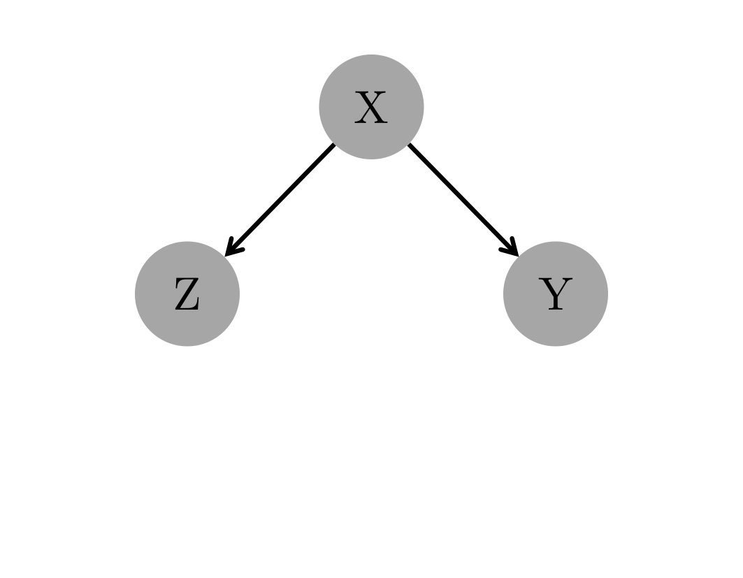 Figure 1
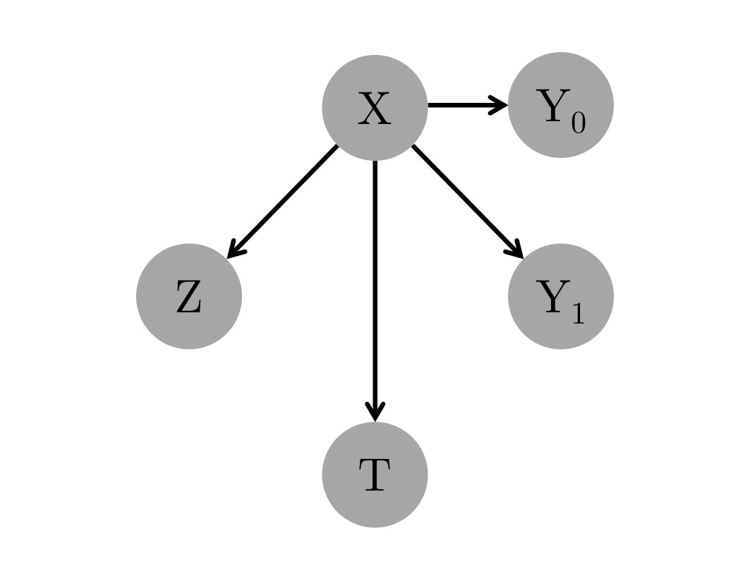 Figure 1
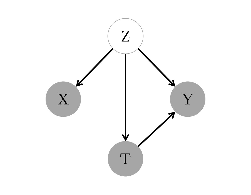 Figure 1
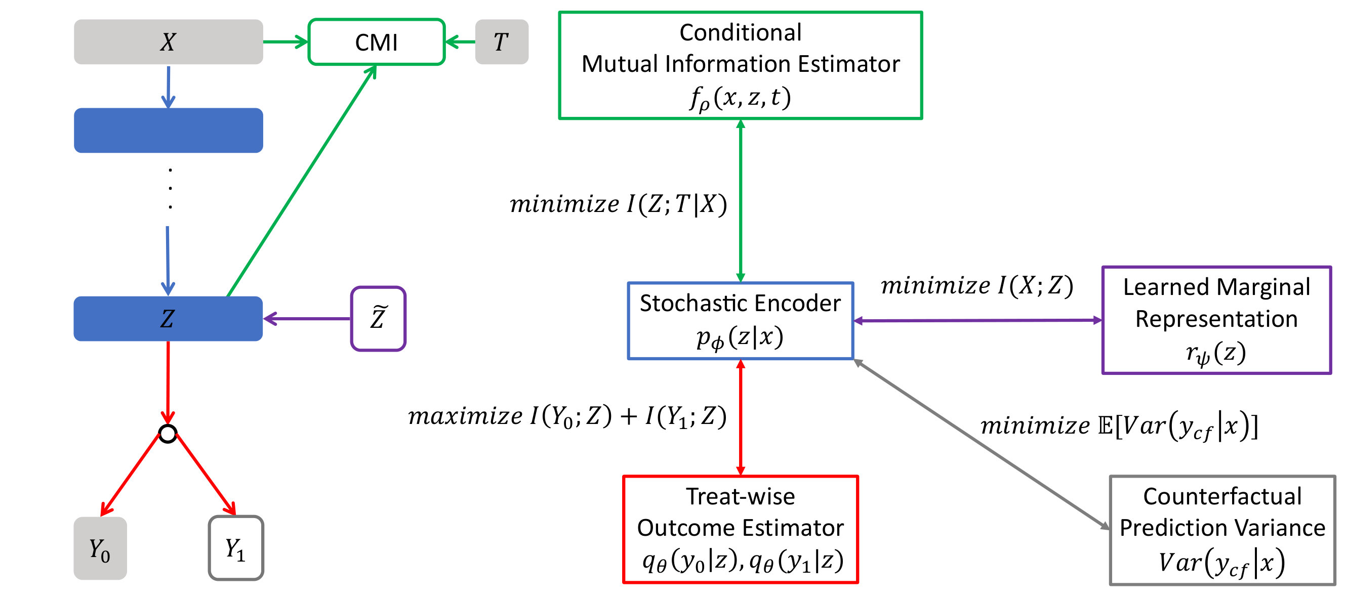 Figure 2
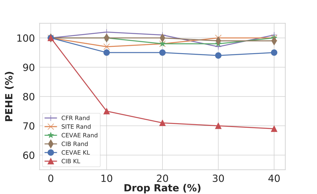 Figure 3
| Dataset | IHDP() | Jobs() | Twins(AUC) |
|---|---|---|---|
| TARNET | |||
| CFR-M | |||
| CFR-W | |||
| CEVAE | not reported | ||
| SITE | |||
| CIB |
| Dataset | IHDP() | Jobs() | Twins(AUC) | |||
|---|---|---|---|---|---|---|
| In-sample | Out-sample | In-sample | Out-sample | In-sample | Out-sample | |
| CIB | ||||||
| w/o MIGDR | ||||||
| w/o CPVR | ||||||
| No regularizer | ||||||
| Dataset | IHDP() | Jobs() | Twins(AUC) |
|---|---|---|---|
| OSL/LR1 | |||
| OSL/LR2 | |||
| HSIC-NNM | |||
| PSM | |||
| -NN | |||
| BNN | |||
| TARNET | |||
| CFR-M | |||
| CFR-W | |||
| GANITE | not reported | ||
| CEVAE | not reported | ||
| SITE-M | |||
| SITE-W | |||
| SITE | |||
| CIB |
| Dataset | IHDP() | Jobs() | Twins(AUC) |
|---|---|---|---|
| OSL/LR1 | |||
| OSL/LR2 | |||
| HSIC-NNM | |||
| PSM | |||
| -NN | |||
| BNN | |||
| TARNET | |||
| CFR-M | |||
| CFR-W | |||
| GANITE | not reported | ||
| CEVAE | not reported | ||
| SITE-M | |||
| SITE-W | |||
| SITE | |||
| CIB |
Peer Reviews
No public reviews on file for this paper yet. If you reviewed it on a platform where reviews are public (OpenReview, ICLR, NeurIPS, ICML), you can paste yours below so the community can read it here.
Videos
No videos yet. Explain this paper in a talk, walkthrough, or lecture? Add one.
Taxonomy
TopicsAdvanced Causal Inference Techniques · Bayesian Modeling and Causal Inference · Domain Adaptation and Few-Shot Learning
Reliable Estimation of Individual Treatment Effect with Causal Information Bottleneck
Sungyub Kim1, Yongsu Baek1, Sung Ju Hwang1,2, Eunho Yang1,2
KAIST1, AItrics2, South Korea
{sungyub.kim, yongsubaek, sjhwang82, eunhoy} @kaist.ac.kr
Abstract
Estimating individual level treatment effects (ITE) from observational data is a challenging and important area in causal machine learning and is commonly considered in diverse mission-critical applications. In this paper, we propose an information theoretic approach in order to find more reliable representations for estimating ITE. We leverage the Information Bottleneck (IB) principle, which addresses the trade-off between conciseness and predictive power of representation. With the introduction of an extended graphical model for causal information bottleneck, we encourage the independence between the learned representation and the treatment type. We also introduce an additional form of a regularizer from the perspective of understanding ITE in the semi-supervised learning framework to ensure more reliable representations. Experimental results show that our model achieves the state-of-the-art results and exhibits more reliable prediction performances with uncertainty information on real-world datasets.
1 Introduction
Estimating individual-level treatment effect (ITE) , which infers causality between a treatment and an outcome from observational data, is one of the fundamental problems in machine learning and is essential in various applications such as healthcare [29, 12, 1], political science [30, 21], and online advertisement [23, 34] to name a few. In order to accurately deduce the causality between a treatment and an outcome, it is necessary to predict the outcome of each treatment correctly for each individual data point. However, in the usual (or almost all) observational studies, each data point is only allowed to receive one treatment out of several options, and the results for other unselected treatments do not even exist in the data. Hence, this ITE problem is connected to counterfactual questions [18] like “If the patient received other prescriptions, would the patient’s disease progress differently?”. A naive approach for this is to predict counterfactual outcomes that have not been observed, using the model trained only on observed factual data. One implicit assumption of such an inference is that the input distributions of the treatment and control groups (in case of two options) should be identical. It is known, however, that a bias may exist in the selection of treatments, unless the data are obtained in a rigorously randomized controlled trial, leading to a covariate shift in the ITE problem.
To overcome this difficulty, previous works focus on a representation learning approach. A common central idea in this vein is to learn the feature extractor by which any discrepancy between the treatment and the control becomes smaller in the learned representation space than in the original covariate space. Almost all existing works based on this representation learning approach for ITE can be seen as a way of finding balanced and maximally expressive representation that could be simultaneously used in the prediction of factual and counterfactual outcomes.
Motivated by the recent success of information bottleneck in several domains [3, 2, 28], in this paper we propose a causal information bottleneck (CIB) that additionally pursue maximal compressiveness between the representation for ITE prediction and the observed covariate, on top of previously considered balance and maximal expressiveness. By learning with information bottleneck principles [32], not only can one learn an ideal representation that can better predict the counterfactual outcomes, but one can also gain additional (but more important in some sense) effects. Specifically, earlier work [3] showed that models learned with information bottleneck objective are more robust to overfitting and adversarial attacks than models learned through other forms of objectives or regularizations. This occurs because the representation found through information bottleneck tries to ignore as much information as possible from the covariate and hence idiosyncratic perturbations cannot easily pass through an information bottleneck. In addition to improving generalization, models learned by IB principals are empirically shown to be well calibrated providing meaningful uncertainty about their predictions [2]. In the same context, one can expect that the proposed CIB naturally inherits such benefits of IB. Toward this, we experimentally confirm that CIB yields significantly better results against baselines on the scenario where the models are allowed to say “I don’t know” on instances that are different from the training data and hence they are not sure. It is one of the most important desiderata to provide accurate uncertainty on their predictions since most tasks that consider the counterfactual inference are irreversible and mission-critical problems with serious consequences.
Main contributions.
The main contributions of this paper are as follows:
- •
We introduce a graphical model for causal inference on which we can apply the information bottleneck (IB) principle for reliable individual treatment effect (ITE) estimations. The proposed principle is formulated as a simple optimization problem that can be efficiently solved with stochastic gradient methods [19] and a reparameterization trick [20].
- •
Along with the standard information bottleneck, we propose to use two additional regularizations, one that emerges naturally by the graph structure and another inspired by semi-supervised learning literature, to help learning representations for ITE.
- •
We validate our model on three standard benchmark datasets and show that our model significantly outperforms with well-calibrated uncertainty for the scenario where the models are allowed to say “I don’t know”.
2 Background and Setup
Individual Treatment Estimation (ITE)
Here, we denote the set of possible covariates by and the set of possible outcomes by . We focus on a binary treatment scenario that selects one among the treat/control options, just for simplicity. For convenience of the notation, we use [math] to denote the control and to denote the treat, that is, the space of treatment is . For example, let be a covariate describing the features of patient . If the patient chooses to receive some treatment, , otherwise . The actual patient progression variable (e.g. blood pressure, blood sugar) after selecting the medical care becomes . Such a set of factual data can be expressed as for patients. Similarly, the counterfactual data can be expressed as , however there is no value available in the observational data. The individual treatment effect (ITE) that we want to estimate is a conditional expected difference between the treatment outcome and the control outcome given covariate , \tau(x_{i})=\mathbb{E}\big{[}y_{i}^{(1)}-y_{i}^{(0)}|x_{i}\big{]}. A commonly used metric to evaluate the performance of ITE estimators is the expected Precision in Estimation of Heterogeneous Effect (PEHE) [14], which is defined as \epsilon_{PEHE}=\mathbb{E}_{x}\big{[}\big{(}\tau(x_{i})-\hat{\tau}(x_{i})\big{)}^{2}\big{]}. Here, is the predicted difference by the model.
As several works on causal inference including [18, 29, 35] did for justifiability of counterfactual prediction, we also assume throughout the paper the following two conditions of the Rubin-Neyman causal model [4, 29]:
- •
(Overlap) ,
- •
(Conditional ignorability) Y\rotatebox[origin={c}]{90.0}{\models}T|X.
The overlap assumption here requires that all patients have a strictly greater than [math] probability of receiving all treatments. This assumption is necessary to ensure that each patient has both possibilities of being treated or controlled so that so that ITE can be meaningfully estimated. The assumption of conditional ignorability implies that the covariate has sufficient information about the common effects of treatment decisions and outcomes. Therefore, it is also referred to as an unconfoundedness assumption [27]. This unconfoundedness assumption is necessary to make the estimation of ITE identifiable [16].
Information Bottleneck (IB) principle
The information bottleneck principle was first proposed in [32]. The trade-off between maximal expressiveness and maximal compressiveness in the information bottleneck theory is expressed by the following expression, which contains two mutual information terms : one between input and representation and the other between representation and output :
[TABLE]
The classical information bottleneck assumes the graphical model shown in Figure 1(a) and computes by sampling from stochastic encoder given input. In general, it is known that the information bottleneck principle is difficult to pursue since a precise estimation of the mutual information is intractable. However, recent works such as those focusing on variational approximation [3] and adversarial learning [5] proposed efficient techniques to approximate mutual information and confirmed that information bottleneck is an effective regularization methodology robust to observation noise, hence providing better generalization performance and resilience against adversarial attacks and so on.
3 Causal information bottleneck (CIB)
It is important to note that even under the conditional ignorability above, the covariate might have information irrelevant to both and in many real problems. Such noise in covariates cause problems such as overfitting. Since in the main application fields of causal inference such as health care and political science, it is hard to collect huge number of training data, and moreover they are usually irreversible mission-critical problems, we need a systematic way of removing such noise present in the covariate and having a reliable representation for predictions.
Toward this, in this section we propose an information bottleneck framework for causal inference. We extend the graphical model in Figure 1(a) into the form of Figure 1(b) to incorporate variables on treatment and factual/counterfactual outcomes. Unlike the graphical models to capture data generation process with hidden confounder (for example, CEVAE [24] in Figure 1(c)), the graphical model of CIB directly extends the information bottleneck to causal inference task, to find some good representation in the discriminative setting. Note that treatment and outcome are conditionally independent given covariate , which is a sufficient condition for the conditional ignorability of the Rubin-Neyman causal model. Under the graphical model shown in Figure1(b), we propose the information bottleneck principle for the causal model:
- •
(Maximal Expressiveness) representation should have high mutual information with treatment outcome .
- •
(Maximal Compressiveness) representation should have low mutual information with covariate .
These principles can be expressed as the following optimization problem, with a tunable Lagrange multiplier :
[TABLE]
The first term in the objective (1), maximal expressiveness of for control outcome , can be calculated by the following variational approximation [3]:
[TABLE]
where is a variational approximation of the conditional distribution and is the entropy of the random variable . The inequality (2) follows from the non-negativity property of the Kullback Leibler (KL) divergence:
[TABLE]
Now (3) can be calculated as follows with a stochastic encoder :
[TABLE]
This follows from the fact that under the graph structure Figure 1(b).
Here, additional difficulty arises in computing (4) due to the nature of observational data; we must marginalize over the entire population , but we know only for the conditional population . To overcome this issue, we can further derive (4) under the overlap assumption above:
[TABLE]
At this point we introduce the score classifier to estimate the probability of treatment from data and define the loss:
[TABLE]
We can derive the variational bound for the mutual information between and in a similar way.
On the other hand, the last term in (1), the maximal compressiveness, can be computed as a seamless extension of variation approximation for standard IB [3]: where is a variational approximation of .
Meanwhile, the graphical model of Figure 1(b) assumes that representation is conditionally independent of the treatment given covariate . Without additional constraint, this assumption can not be satisfied with a stochastic encoder . Hence, we introduce a novel technique referred to as mutual information guided disentangling that will be explained in the next subsection. Furthermore, the ITE estimation where we are asked to predict unlabeled counterfactual outcomes, may be understood under the semi-supervised learning framework. Based on this interpretation, we apply predictive variance regularization, a popular method in semi-supervised learning [17], for counterfactual prediction.
Mutual Information Guided Disentangled Representation (MIGDR)
In order to encourage according to our graphical structure, we minimize the conditional mutual information between them,
[TABLE]
Since applying the variational approximation technique as above is not trivial in this case due to the conditional expectation, we resort to the Donsker-Varadhan representation-based methodology [9]. According to the Donsker-Varadhan representation, the above KL divergence can be expressed as follows [5],
[TABLE]
where is a scalar-valued function whose two expectations are finite. As proposed in [5], this can be approximated efficiently by estimating auxiliary neural network with parameter . This additional network discriminate between samples from joint distribution and samples from product distribution . From , one can efficiently minimize conditional mutual information between representation and target label by maximizing
[TABLE]
More details are provided in the appendix.
Counterfactual Predictive Variance Regularization (CPVR)
Predictive variance regularization, a method commonly used for semi-supervised learning, adds variance minimization to the predictive distribution of unlabeled data as a regularization term [17]. In the regularized Bayesian framework, this method includes the intuition that an unlabeled sample is close to the labeled sample in the representation space [1, 17]. In this paper, we provide an inductive bias so that counterfactual predictions generated by stochastic encoder are consistent to each other.
[TABLE]
The predictive variance regularization is similar to the nearest neighbor methodology frequently used in counterfactual predictions [18, 7, 22] in that both provide an approximate target for counterfactual data. However, predictive variance regularization uses the predictions of learned networks, while nearest based methods propagate factual data to unlabelled counterfactual outcomes. The nearest neighbor method can be a good approximation when the reference data is sufficient, but the predictive variance regularization can provide better inductive bias if there is little data to calculate nearest neighbors. We use the gradient information of CPVR only to update the parameters of stochastic encoder as in [1, 17].
Overall, the final objective of CIB is described as (with graphical description in Figure 2)
[TABLE]
where involves the following optimization problem
[TABLE]
4 Related Works
Balanced representation for causal inference
The idea of balancing the representation between heterogeneous samples is a commonly used idea in the field of unsupervised domain adaptation [11, 33, 15]. This idea comes from the concept of -divergence in [6]. It is proposed in [18, 29] that this idea can be applied to counterfactual inference. The mutual information guided disentangled representation proposed in this paper is different to these works in that the target label is regularized to be conditionally independent when the representation and covariate are given.
Properly exploiting the local structure of each covariate in learning balanced representation is an important issue in the ITE. The most common idea is known as the nearest neighbor matching (NNM), which finds opponent treatment data for each covariate [18, 22, 35]. The predictive variance regularization is also considered to find some kernel in [1, 17]. In contrast to these studies, we propose to apply this predictive variance regularization to the learning of stochastic encoders. Recently, [10] also proposed the balancing method in an adversarial way for causal inference.
Generative models for causal inference
The stochastic encoder of CIB can be understood as a generative model in that it samples representations satisfying the information bottleneck principle for causal inference. The variational information bottleneck [3] is known as the supervised learning version of -VAE [13]. Despite their similarities on network architectures and loss functions, they have different interpretations; VIB with stochastic encoders variationally approximates the marginal representation distribution and the conditional distribution , but VAE with the prior and sample generators approximates the posterior distribution . This difference is related to regularizations on . Since our model is the natural extension of VIB for causal inference, it inherits this property and has a similar connection to CEVAE [24].
Information bottleneck principle is used for causal inference by recent parallel work [25]. A graphical structure for CEIB [25] assumes that the representation directly affects to outcome . On the other hand, CIB naturally extends the standard information bottleneck principle and inherits its benefits. This difference between CIB and CEIB influences the details of architecture selections and objective functions.
5 Experiment
We evaluate CIB on three real-world datasets used in the existing literature [18, 29, 24]. Due to the space constraints, we defer descriptions on datasets and evaluation metrics to the appendix.
Baselines
We compare our method against classical regression methods, nearest neighbor based methods and representation learning based methods. Classical regression methods involve Ordinary Least Squares with treatment as a feature (OLS/LR 1), OLS with separate regressors for each treamtment (OLS-2). Nearest neighbor based methods contain Hilbert-Schmidt Independence Criterion based Nearest Neighbor Matching (HSIC-NNM) [7], Propensity Score Match with logistic regression (PSM) [26] and -nearest neighbor (-NN) [8]. Representation learning based methods contain Balanced Neural Network (BNN) [18], Treatment-Agnostic Representation Network (TARNET), Counterfactual regression with MMD/Wasserstein metric (CFR-M/W) [29], Generative Adversarial Nets for inference of ITE (GANITE) [36], Causal Effect Variational Autoencoder (CEVAE) [24] and local Similarity preserved Individual Treatment Effect (SITE) [35]. We also report the results for SITE with MMD/Wasserstein metric (SITE-M/W). Results in Table 2 and 2 except our model are reported in [36, 24, 35]. We parenthesized the results of CEVAE and GANITE, since their results are based on slightly different setting: 1000 realization for IHDP dataset and 100 realization for Jobs dataset (GANITE).
Implementation
We use a shared encoder for both treat/control data and separate regressors as in TARNET [29]. Using a Gaussian reparameterization trick as proposed in VIB [3], our stochastic encoder predicts mean and standard deviation of conditional Gaussian given covariates. We use the same number of hidden layers for conditional mutual information estimator and encoder. We use single-layered networks for regressors. The score classifier did not improve empirical performance of CIB, and was omitted. More details on implementations are provided in the appendix.
Results
Tables 2 and 2 represent means and standard errors of 10 realizations/splits on three datasets. CIB achieves the best result for in-sample error on Twins dataset and out-sample error on IHDP and Twins datasets. On Jobs datasets, CIB shows the comparable performance to other state-of-the-art models. Tables here only show comparisons against major baselines and full comparisons are provided in the appendix due to the space constraints.
As noted in [35], the results show that the representation learning based methods outperform the classical regression methods and the nearest neighbor based methods. Our CIB method also follows this tendency. Although other representation balancing methods such as BNN [18], CFR [29] and SITE [35] consider group-wise balancing representation, i.e. their regularization for balancing representation is defined for a group of representations, while MIGDR of CIB considers seeks instance-wisely balanced representation. Since CIB adds an auxiliary network for balancing representations, it does not suffer from calculating the Sinkhorn divergence in CFR-W or choosing optimal kernel in CFR-M. Also, CIB does not need to hold hard examples to consider local similarity unlike SITE.
Uncertainty calibration with information bottleneck penalty
Since the representation of CIB is modeled as conditional Gaussian, we can measure how generated representation given covariate is rare compared to marginal representation as . Therefore, if we average this with sampled representation as , we can interpret this term as an indicator for how much the covariate is out-of-distribution (OOD) sample for entire population [2]. In order to explicitly benefit this property, we consider the scenario in this experiment where models are allowed to answer “I don’t know” for uncertain inputs.
In Figure 3, we show our results on removing top % uncertain samples for IHDP datasets. Since CEVAE [24] can also measure for confounder , we also remove uncertain samples based on this KL divergence (denoted as "CEVAE KL"). However, since the predictive variances are unavailable for other methods, we just drop % samples randomly for them. As Figure 1 shows, only CIB quickly finds and drops samples on which it is not sure.
Ablation Study
We proposed two additional regularizations above, MIGDR and CPVR on top of basic CIB framework. Here, we confirm our additional regularization is critical to empirical success of our model. Toward this, we compare our CIB against CIB without MIGDR, CIB without CPVR and CIB with no additional regularization on three datasets. Table 3 summarizes the results. The CPVR regularization is critical to results for IHDP dataset, while both MIGDR and CPVR are important for other datasets.
6 Conclusion
We introduced a novel framework CIB for estimating ITE by extending information bottleneck. On the top of information bottleneck framework, we proposed two additional regularizations to learn more reliable representation. We confirmed CIB method performs comparable to state-of-the-art models and reliable in detecting how much given covariate is out-of-distribution (OOD) sample for entire population . This property of CIB is critical to mission-critical applications of causal inference.
Appendix A Details on MGIDR
As mentioned in main text, conditional mutual information between and can be represented as
[TABLE]
where is a scalar-valued function whose two expectation are finite. Due to the universal approximation properties of the neural network, this statistic is strongly consistent when we approximate with neural networks without optimizing on the infinite dimensions[5]. Learning to maximize the mean difference between the two distributions is similar to learning discriminators in generative adversarial learning. Because it is less important to calculate the exact mutual information in this paper, we optimize the statistic network using a zero-centered gradient penalty[31], which is more stable and known to be capable of greater generalization performance outcomes. Moreover, finding the optimal for each covariate is inefficient because doing so requires the estimation of several functions. Therefore, the statistic network is learned with amortized inference by considering conditionally.
Appendix B Details on Experiments
Datasets
To evaluate the proposed CIB, we use three real-world datasets used to evaluate the existing methodologies[18, 29, 24]. The covariates of Infant Health and Development Program (IHDP) dataset are from real-world randomized controlled trial experiment. By removing some of the treated observations of RCT dataset, the IHDP dataset intentionally involves selection bias and is used as benchmark data for ITE researches. More details are given in [14]. The data consists of 25 dimensions 747 covariates . We split train/validate/test 10 realization of simulated data with 63/27/10 ratio as proposed in [35]. Jobs dataset [21] is a mixed observations based on the National Support Work program with observational study [30]. The covariate of Jobs dataset consists with 17 dimension 3212 instance. Since this dataset consists of one realization without repeated simulation, we experimented with 10 times train/validation/test split with 56/24/20 ratio as suggested in [29]. The Twins dataset was used as the benchmark data of counterfactual inference in for the first time in [24]. This data is based on the twins born in the USA in 1989-1991. As in [35], we focus on the same sex twin-pair less than 2000g. The covariate is a 40-dimensional data consisting of parents, their condition at the time of their pregnancy, and birth information. We used the identical data preprocessing as suggested in [35].
Performance Metrics
In the case of IHDP datasets where all control/treat outcomes are known for each covariate, we use the expected Precision in Estimation of Heterogeneous Effect (PEHE). Since there exists only factual outcome for a given covariate, it is intractable to calculate the PEHE score in Jobs data. In order to evaluate the performance of the learned model, [29] defined a policy based on the learned model as follows.
[TABLE]
[TABLE]
We estimate this for the randomized subset of Jobs dataset as
[TABLE]
where , , ,, . Finally, for the Twins dataset, we report area under ROC (AUC) for counterfactual prediction as proposed in [24].
We measure the in-sample error with both train and valid data and out-sample error with only test data. This convention follows [18, 29, 35]. Since in-sample evaluation metric is non-trivial, as we never observe the ITE for any unit, we report in-sample results.
We measure the in-sample error with both train and valid data and out-sample error with only test data. This convention follows [18, 29, 35]. Since in-sample evaluation metric is non-trivial, as we never observe the ITE for any unit, we report in-sample results.
Implementation
For cross-validation, We search to optimize the number of hidden layers in encoder (), the dimension of layers ( and the regularization coefficients (). We use Adam[19] with for learning rate and . We train 2000 iterations with early stopping as [29, 35]. Experiments in this paper are conducted on a cluster with Intel Xeon E5 2.2GHz CPU, 4x Nvidia Titan Xp GPU and 256GB RAM.
Appendix C Full Experiment Result
Bold font indicates that the mean belongs to 95% confidence interval of the best performing model on each dataset.
The reference list from the paper itself. Each links out to its DOI / PubMed record.
- 1Alaa and van der Schaar [2017] Alaa, A. M. and van der Schaar, M. (2017). Bayesian inference of individualized treatment effects using multi-task gaussian processes. In Advances in Neural Information Processing Systems 30 , pages 3424–3432.
- 2Alemi et al. [2018] Alemi, A. A., Fischer, I., and Dillon, J. V. (2018). Uncertainty in the variational information bottleneck. ar Xiv preprint ar Xiv:1807.00906 .
- 3Alemi et al. [2017] Alemi, A. A., Fischer, I., Dillon, J. V., and Murphy, K. (2017). Deep variational information bottleneck. In ICLR .
- 4B. Rubin [1974] B. Rubin, D. (1974). Estimating causal effects of treatments in randomized and nonrandomized studies. Journal of Educational Psychology , 66(5):688–701.
- 5Belghazi et al. [2018] Belghazi, M. I., Baratin, A., Rajeshwar, S., Ozair, S., Bengio, Y., Courville, A., and Hjelm, D. (2018). Mutual information neural estimation. In Proceedings of the 35th International Conference on Machine Learning , pages 531–540.
- 6Ben-David et al. [2010] Ben-David, S., Blitzer, J., Crammer, K., Kulesza, A., Pereira, F., and Vaughan, J. W. (2010). A theory of learning from different domains. Machine learning , 79(1-2):151–175.
- 7Chang and Dy [2017] Chang, Y. and Dy, J. G. (2017). Informative subspace learning for counterfactual inference. In Thirty-First AAAI Conference on Artificial Intelligence .
- 8Crump et al. [2008] Crump, R. K., Hotz, V. J., Imbens, G. W., and Mitnik, O. A. (2008). Nonparametric tests for treatment effect heterogeneity. The Review of Economics and Statistics , 90(3):389–405.