Stochastic learning control of inhomogeneous quantum ensembles
Gabriel Turinici (CEREMADE, IUF)

TL;DR
This paper explores stochastic optimization methods like stochastic gradient descent and Adam for controlling inhomogeneous quantum ensembles, demonstrating their effectiveness in high-dimensional uncertainty scenarios.
Contribution
It introduces stochastic search procedures for quantum control that handle high-dimensional uncertainties, improving upon fixed-grid approaches.
Findings
Algorithms perform well against benchmarks
Effective in 3D and 6D parameter spaces
Handle high-dimensional uncertainties efficiently
Abstract
In quantum control, the robustness with respect to uncertainties in the system's parameters or driving field characteristics is of paramount importance and has been studied theoretically, numerically and experimentally. We test in this paper stochastic search procedures (Stochastic gradient descent and the Adam algorithm) that sample, at each iteration, from the distribution of the parameter uncertainty, as opposed to previous approaches that use a fixed grid. We show that both algorithms behave well with respect to benchmarks and discuss their relative merits. In addition the methodology allows to address high dimensional parameter uncertainty; we implement numerically, with good results, a 3D and a 6D case.
Click any figure to enlarge with its caption.
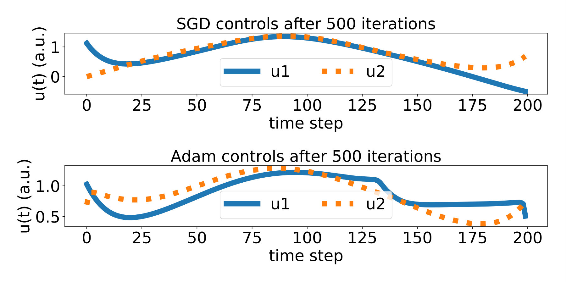 Figure 1
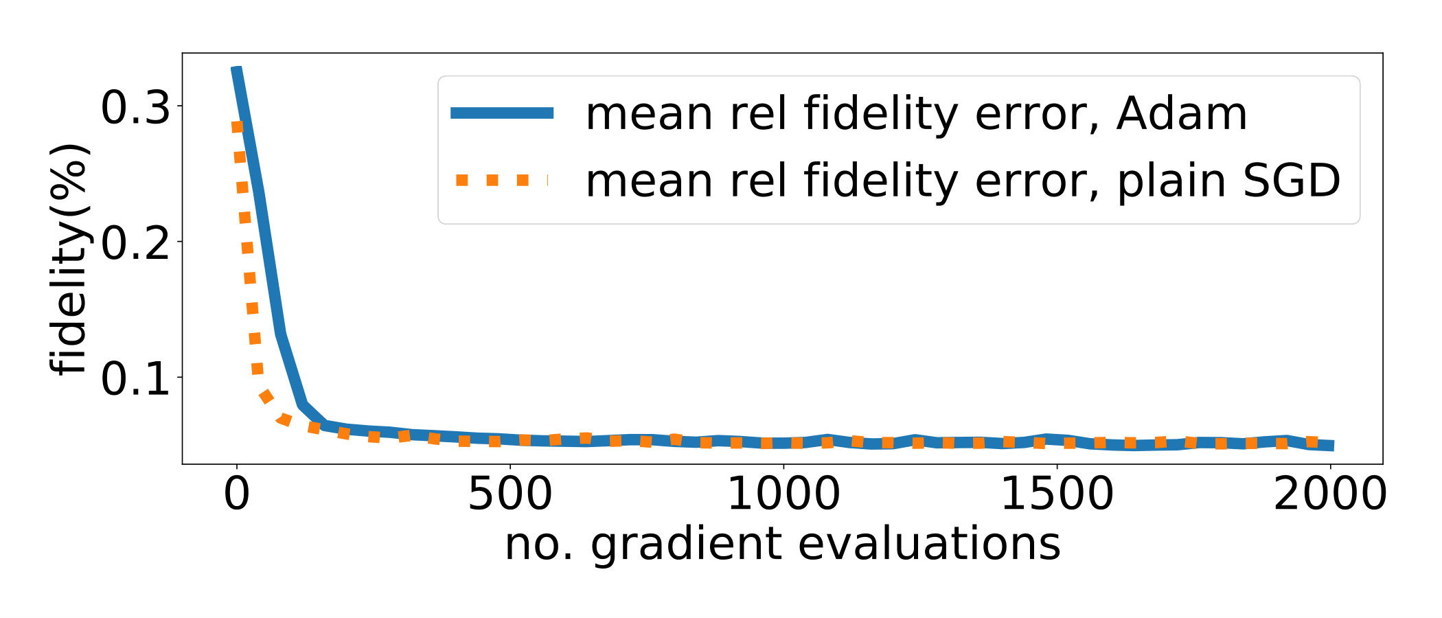 Figure 2
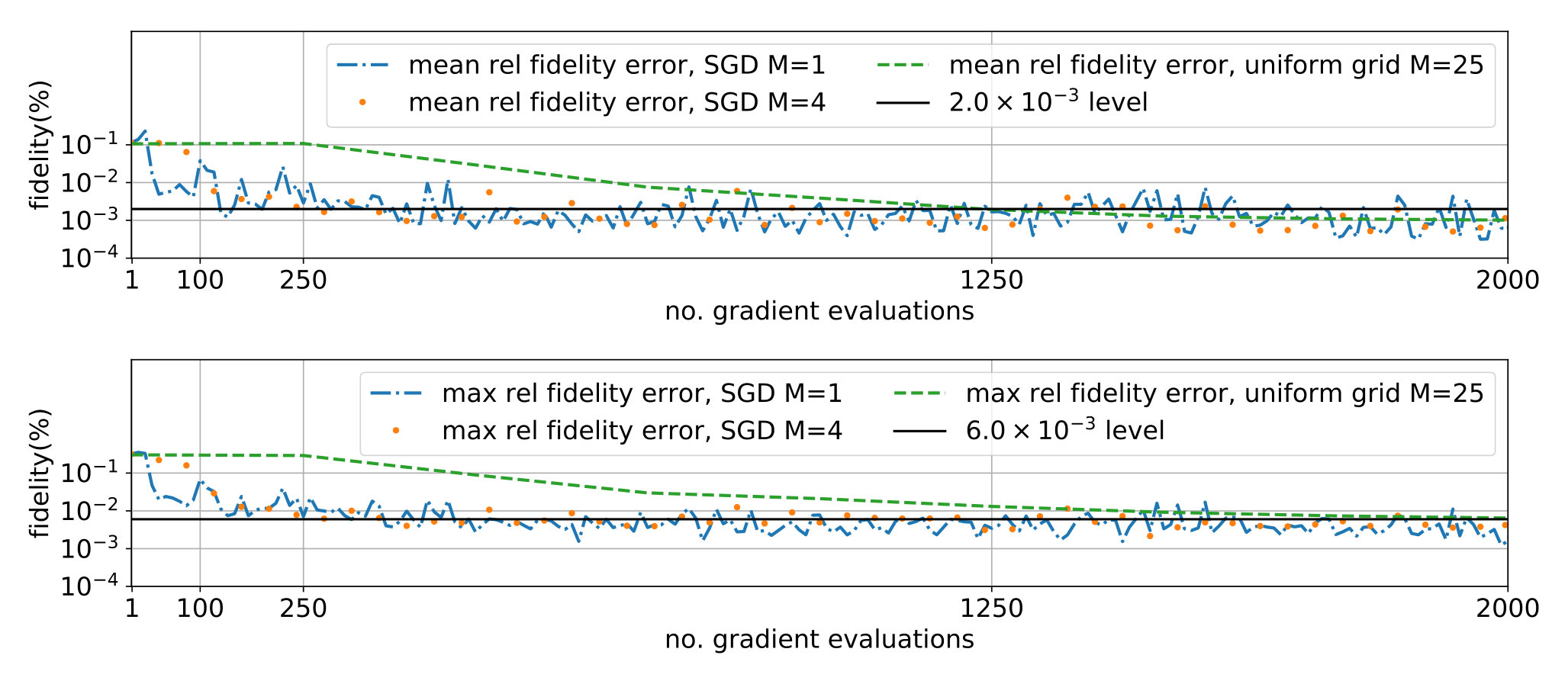 Figure 3
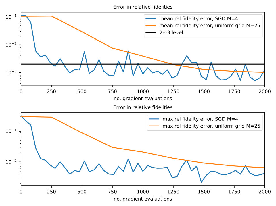 Figure 4
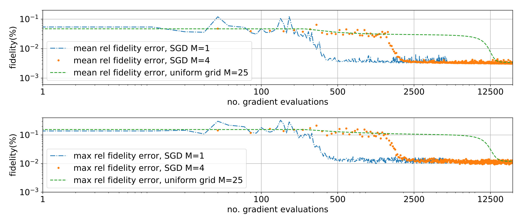 Figure 5
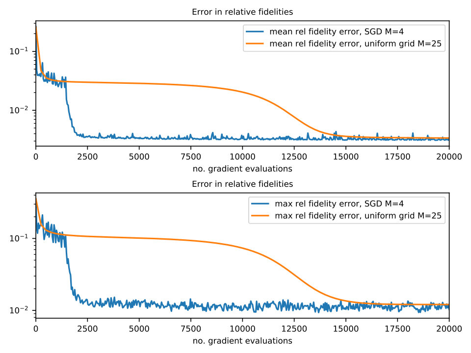 Figure 6
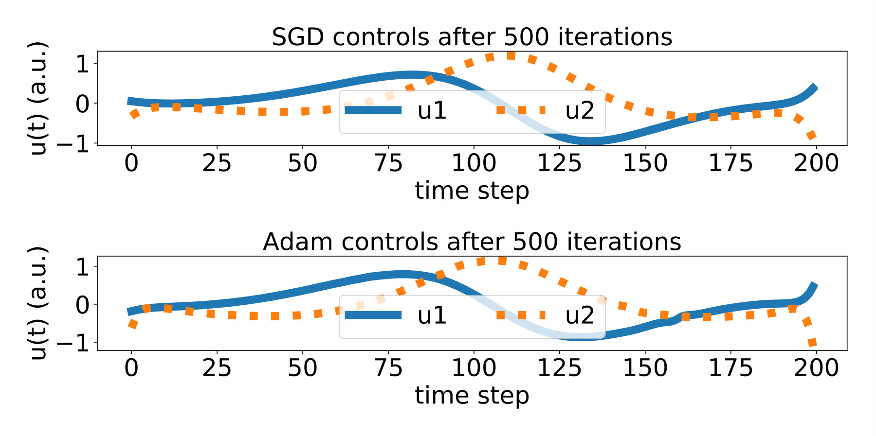 Figure 7
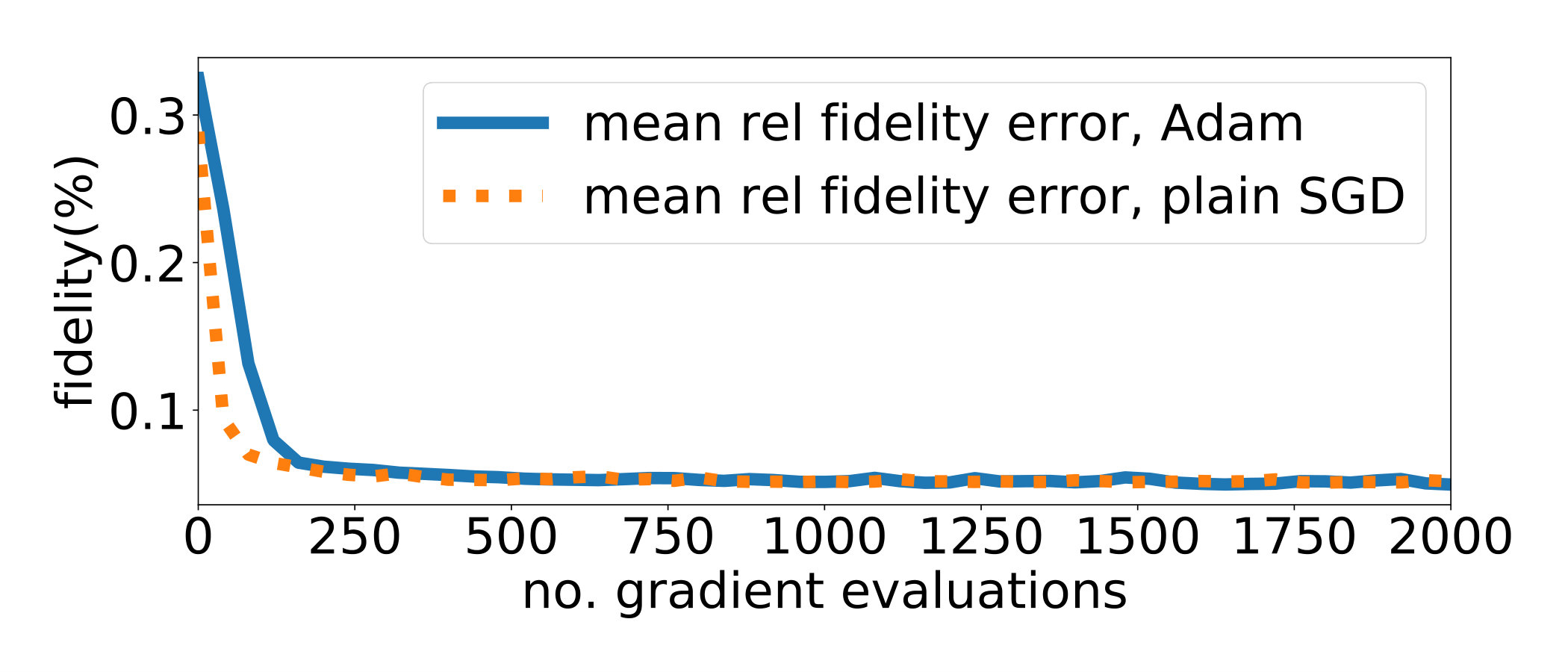 Figure 8
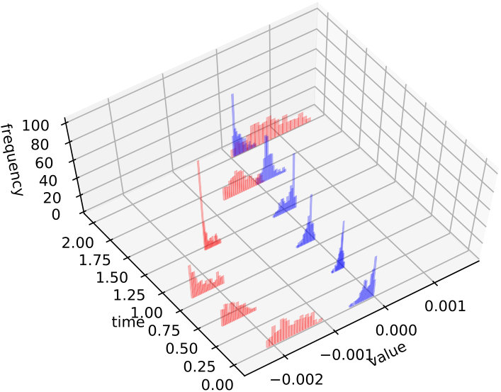 Figure 9
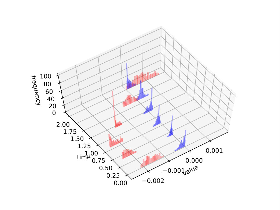 Figure 10
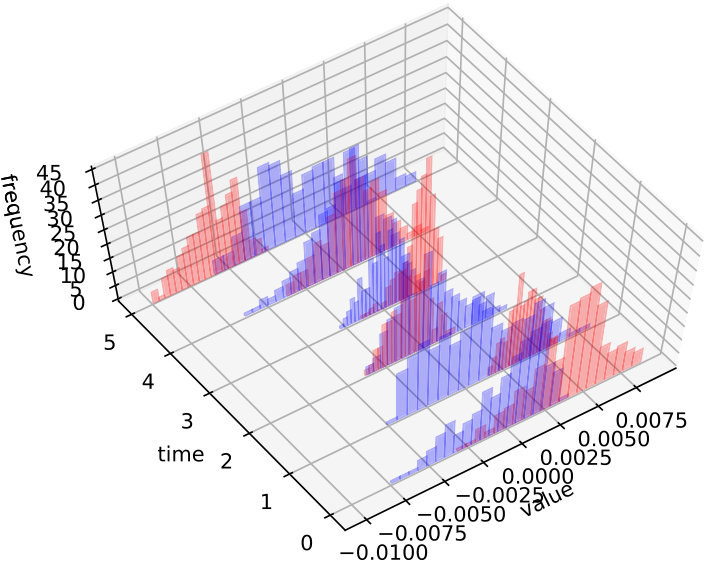 Figure 11
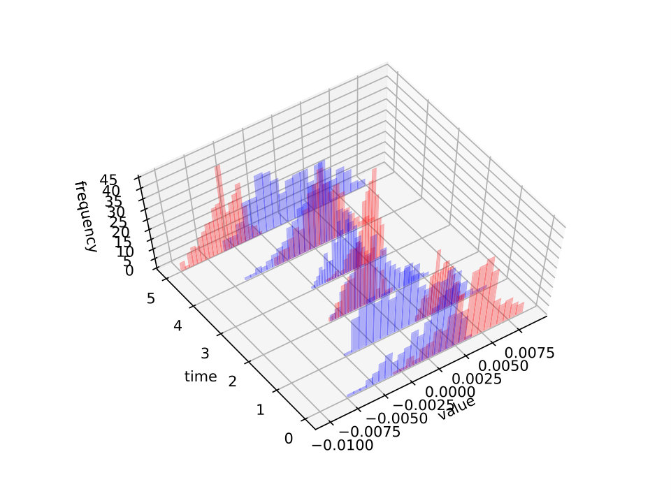 Figure 12
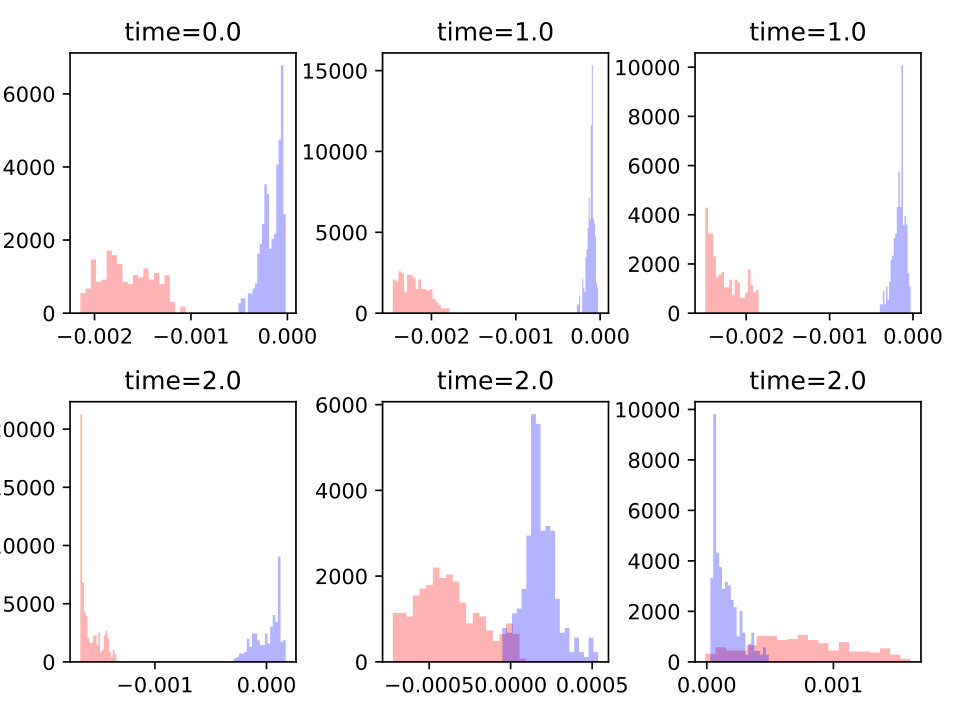 Figure 13
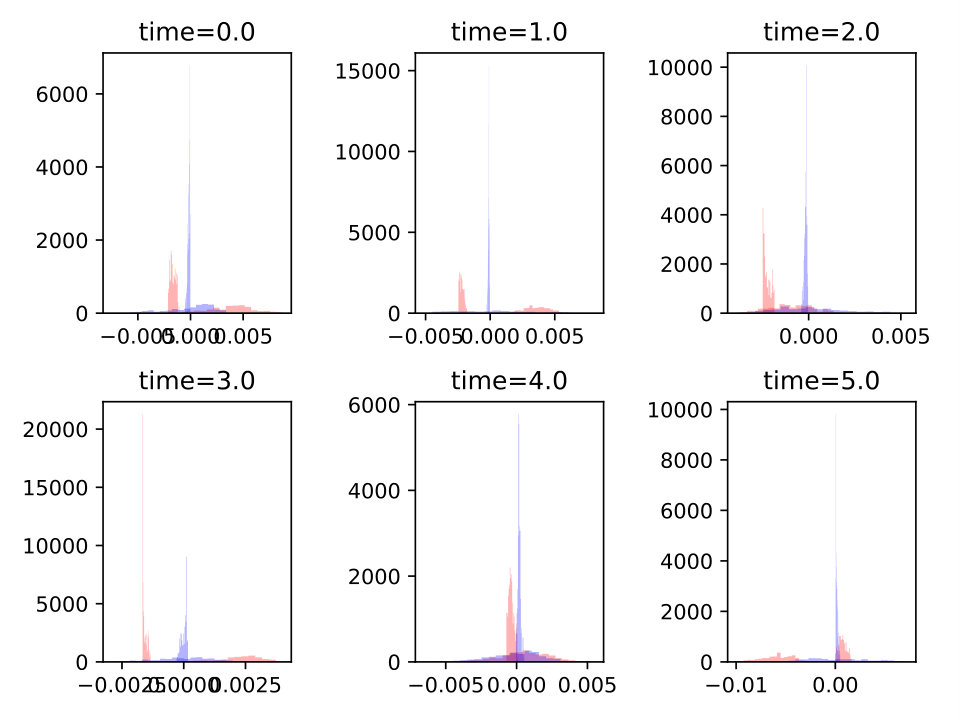 Figure 14
Peer Reviews
No public reviews on file for this paper yet. If you reviewed it on a platform where reviews are public (OpenReview, ICLR, NeurIPS, ICML), you can paste yours below so the community can read it here.
Videos
No videos yet. Explain this paper in a talk, walkthrough, or lecture? Add one.
Taxonomy
MethodsAdam
Stochastic learning control of inhomogeneous quantum ensembles
Gabriel Turinici
IUF - Institut Universitaire de France
CEREMADE, Université Paris Dauphine - PSL Research University
(Oct 2019)
Abstract
In quantum control, the robustness with respect to uncertainties in the system’s parameters or driving field characteristics is of paramount importance and has been studied theoretically, numerically and experimentally. We test in this paper stochastic search procedures (Stochastic gradient descent and the Adam algorithm) that sample, at each iteration, from the distribution of the parameter uncertainty, as opposed to previous approaches that use a fixed grid. We show that both algorithms behave well with respect to benchmarks and discuss their relative merits. In addition the methodology allows to address high dimensional parameter uncertainty; we implement numerically, with good results, a 3D and a 6D case.
1 Introduction
Quantum control is a promising technology with many applications ranging from NMR [12] to quantum computing [15] and laser control of quantum dynamics [7]. The controlling field encounters many molecules which although identical in nature may interact differently with the incoming field because of e.g., different Larmor frequencies or rf attenuation factors (in NMR spin control or quantum computing, see [19, 29, 35, 22, 13, 17]), different spatial profile (see [24]) or other parameters (see [36, 8, 10]). For obvious practical reasons, it is of paramount importance to ensure that the control quality is robust with respect to this heterogeneity. Thus the quantum control problem involves a unique set of driving fields , the same for all molecules in the ensemble, however each molecule is described by a set of parameters and the control outcome depends on both and ; the goal can be expressed as the maximization of the control quality averaged over . A different view is when the variability is not due to the presence of many different molecules but when uncertainties in the control implementation require to devise a field robust to fluctuations in those parameters.
A first natural question is whether this is at all possible, i.e., if a single field can drive several distinct molecules to a common target; the answer is given by the theory of ensemble control controllability, see [31, 5, 19, 4, 6] and is in general positive. However the theory does not explain how to find the control (except under specific regimes, see [2]). To do so, different algorithms have been proposed: the pseudo-spectral approach of Li et al. [20, 28, 21] consider spectral and/or polynomial representations of the control problem in 2D (); Wang considers iterative procedures based on sampling [32]; the learning approach of Chen et al. [8] and Kuang et al. [18] (the latter in the context of time-optimal control) consider a fixed uniform grid over the inhomogeneous parameter space and was tested for . Finally, Wu and al. [33] find robust controls using uniform grids in 2D and 3D ().
In all these works there is always a fixed grid (or fixed sampling) involved when the control is searched. The rationale behind this idea is that a fixed grid makes the search more stable and a good choice of the grid is enough to describe efficiently the mean performance of the control over the parameter space in the spirit of a quadrature formula for the average over . This is coherent with results from the approximation theory which inform that convergence is of order , with respect to the number of grid points; however the same formula indicates a bad scaling with respect to . To address this curse of dimensionality and also explore the nature of the search landscape, we take here a different view: at each control iteration we use a new sampling in the spirit of Monte Carlo methods (see [23, Section 7.7]) for computing high dimensional integrals. This will induce slight oscillations in the average but has the advantage to cover the space of inhomogeneity even in high dimensions . A similar approach has been tested independently in a very recent work by Wu and al. [34] for a two-dimensional example and promising results were obtained; see Section 2.2 for comments on the differences between the two approaches. The procedure we propose is detailed in the next section and the numerical results are the object of Section 3.
2 Algorithms for ensemble quantum control
We consider a control acting on a molecule part of a larger ensemble. Each molecule is completely characterized by some inhomogeneity parameter obeying a distribution law on (which can be the uniform distribution or any other). All molecules are subjected to the same control during the time interval in order to reach some target.
2.1 Evolution equations
The dynamics of each molecule in the sample is governed by the Hamiltonian through the Schrödinger equation:
[TABLE]
where is the wave-function of the molecule (here and below we set ). Of course, depends on but for notational convenience we omit to write explicitly this dependence from now on. Once a finite dimensional basis is chosen, the state of the quantum system can be represented as
[TABLE]
Denoting the vector of coefficients satisfies the equation:
[TABLE]
where is the representation of the Hamiltonian (including the factor) in the basis , .
Note that same setting also applies to non-linear Hamiltonians e.g. Bose-Einstein condensates (nonlinearity in ), or high order control terms [11, 9] (nonlinearity in ).
The quantum system can also be described in terms of a density matrix ; this matrix is expressed in some basis for operators. Same happens when the molecule is coupled to a bath or when relaxation phenomena are at work, see [1]; in both cases the coefficients of this expansion follow an equation similar to (3).
2.2 Optimization by stochastic gradient descent and Adam algorithms
The control goal is encoded as the minimization, with respect to , of an error, or ”loss” functional depending on the control and the Hamiltonian parameters . When all the ensemble is considered, the following loss functional is to be minimized:
[TABLE]
The stochastic optimization algorithms described below construct an iterative process in order to find the that minimizes (4).
Historically the first to be considered, the stochastic gradient descent algorithm [26] (henceforth called SGD) consists in the following procedure:
In order to accelerate the convergence of the SGD algorithm, several improvements have been proposed (see [27]) among which the Adam [16] variant which proved to be one of the most efficient and very scalable. The difference between Adam and SGD is that Adam uses a different learning rate for each parameter which is tuned as follows: when the uncertainty in the gradient is large the learning rate is taken to be small and contrary otherwise. In order to have a robust estimation for the gradient (in absolute value) a Exponential Moving Average is computed on the fly (see below). It can be described as:
The momentum algorithm used in [34] can be seen as being halfway between SGD and Adam; it is formally a special case of the Adam algorithm for , , and no bias correction step 7 (that is , ). In practice the numerical results are very similar and point in the same direction; in particular we expect that the momentum algorithm is also relevant to high dimensional robust control problems.
3 Numerical results
We test the performance of the algorithms in Section 2.2 for several benchmarks from the literature (or that generalize cases from the literature).
In sections 3.1 and 3.1 we compare the SGD algorithm with a fixed grid sampling method from the literature. Then in section sections 3.3 and 3.4 we compare the SGD wih the Adam algorithm and in Section 3.5 we draw further conclusions concerning stochastic optimization.
In the situations considered below, the goal is to maximize the so-called fidelity denoted . For sections 3.1 and 3.2 this has the formula where is a prescribed target state. But this expression is not differentiable everywhere and numerically it is easier to replace it with its square. Moreover, to express the problem as a minimization, a multiplicative constant is introduced and added to the result in order to have it positive. So the cost functional will be the mean, over of the error in the fidelity squared as in formula (8). On the contrary, when the fidelity is more well behaved as in section 3.3 where or in section 3.4 where the square operation is useless and the cost functional has the form in (11) or (13). However, in all sections, we will plot the error in the fidelity itself; the reason why not plotting the fidelity (instead of the error) is that the error can be very small (as in Section 3.1) and the results are more visible on a logarithmic scale. Note that in some cases the best control cannot attain the target with 100% quality (even for a single molecule). However, for any given value of the parameter , the best attainable performance is known (see [12, 30, 14]) and is denoted . We will therefore consider the fidelity relative to . In all cases the error is computed as the average over random independent parameters , , …, drawn (once for all) from the distribution and has the following expression:
[TABLE]
For sections 3.1 and 3.2 we will also plot the max relative error:
[TABLE]
Finally, in order to compare our algorithm with those from the literature, we take as indicator of the numerical effort the number of gradient evaluations; for instance one iteration of SGD or Adam algorithms count as gradient evaluations. In all situations we used for the Adam algorithm the standard values , , .
3.1 Two level inhomogeneous ensemble
Consider an ensemble of spins as in [8, section III.]. The spins have different Larmor frequencies in the range and the controls () have multiplicative inhomogeneity ; we set and with the previous notations the dynamics corresponds to the equation:
[TABLE]
where , are the coefficients of the wavefunction of the spin system in the canonical basis, as detailed in equation (2).
The initial state of each member of the quantum ensemble is set to ; i.e., , and the goal is to reach the target state ; i.e., . The objective is encoded as the requirement to minimize:
[TABLE]
Here . The total time is is divided into time steps, of length each. The initial choice for the control is .
Several mini-batch sizes and are tested and compared with implementation in [8, section III.A.] where a 2D uniform grid of values for is chosen. In all cases very good convergence results are attained. We plot in Figure 1 the results for , relative to the convergence with the uniform grid. In all cases (, uniform grid) we set ; note that the learning rate was optimized to obtain the best possible results for the fixed grid algorithm and indeed the results are better than those in [8, section III.A.]. But similar conclusions are reached for any value of . An acceleration by a factor of is obtained for both and , essentially due to the fact that each SGD iteration uses only gradient evaluations. Note that the SGD algorithm oscillates but these oscillations can be cured by lowering (or stopping the search) as soon as a good result is obtained. The question of which is the best choice among and is a matter of striking a balance between speed and uncertainty: for the convergence is slightly slower but oscillations are diminished. This behavior is observed, to a larger or lesser extent, in all test cases.
Note that in order to compare our learning rate (for the fixed uniform grid) with that in [8, section III.A.] a multiplicative factor of has to be introduced because our gradient (see Appendix A) contains an extra factor and the coefficient . Thus one should transform to to compare with used in [8].
3.2 A three level atomic ensemble
In this section we test a atomic ensemble from [8, Section IV] which can be written as a -level system with the following dynamics:
[TABLE]
where and have uniform distributions in and , , are the coefficients of the wavefunction of the spin system in the canonical basis, as detailed in equation (2).
The objective is to find a control which drives all the inhomogeneous members from (i.e., ) to (i.e., ); the objective is encoded as the minimization of (8). Here .
We plot in Figure 2 the results for and relative to the convergence with an uniform grid as in [8, section IV.]. In all cases (, uniform grid) we set . The acceleration factor is around for and even larger for (but at the price of larger oscillations too).
3.3 A 3D example: two spin systems without cross-correlated relaxation
As argued before, methods from the literature may have difficulties to address high dimensional parameters, and often limit to two dimensional () inhomogeneity (see however [33, Sec. V.B] for a 3D case). In order to test the full power of our method, we consider two situations that extend cases treated in the literature but have never been treated before. The first test is a three dimensional () example which addresses the coherence transfer between two spins without cross-correlated relaxation, taken from [28, Section III.B.1. eq(15)] (but with an additional inhomogeneity dimension). An example of such a system is an isolated hetero-nuclear spin system composed of two coupled spins corresponding to atoms and . For a general treatment of the relaxation terms and the formulation of this equation see [1]. The spins display control inhomogeneity described by the parameter as above but there is also variation in the relaxation rate and coupling constant, which, denoting results in the dynamical system:
[TABLE]
Let us denote by (here , are the Pauli matrices) the spin operators corresponding to the first spin and the corresponding objects for the second spin. With the usual notations for the Kronecker products, , , , ; the exact derivation of this equation is beyond the scope of this work, see [1, 12, 14] for details. On the other hand also note that the dynamics is not reversible (relaxation is present) and the equations do not correspond to a unitary evolution.
The inhomogeneity is uniformly distributed in . The final time is discretized with uniform time steps. The control is initialized as before. The initial state is encoded as and the target is to minimize the three-dimensional integral:
[TABLE]
Recall that here the fidelity is ; in this case (see [12, 14]) (the worse performance being ). The results are in Figures 3 and 4. Note that although for each taken individually the figure can be attained with a pair (recall ) of suitable control fields, it is unknown whether a unique control pair exists ensuring (relative to ) target yield simultaneously for all . In practice we did not find any, irrespective of the algorithm hyper-parameters such as , the maximum number of iterations etc.; we conclude on one hand that this ensemble is not simultaneously controllable and on the other hand that our procedure improves significantly the robustness of the control with respect to from an initial value of up to . Note that the results from the literature (which for this case only consider 2 dimensional inhomogeneity) do not obtain control either (exact figure is not reported).
3.4 A 6D example: two spin systems with cross-correlated relaxation
We continue here to address new systems that previous methods could not treat. We consider an ensemble of two spin systems with cross-correlated relaxation as in [20, Section III.A.2.], [28, Section III.B.2 eq. (16)] and also [32, Example 3], [1].
The spins display control inhomogeneity described by the parameters and and there is also variation in the auto-correlated relaxation rate , the quotient of the cross-correlation relaxation rate with respect to the auto-correlated relaxation rate and finally, a dispersion in the Larmor frequencies of each spin. Denoting , the dynamical system can be written:
[TABLE]
The vector has real entries and, with the same notations as in equation (10), , , , , , . The relations are similar to that in section 3.3, with the exception that there are two new entries and due to the presence of cross-correlation, see [12, 14, 1] for details of the derivation of the model; the dynamics is not reversible (relaxation is present) nor unitary.
We set ; the total time is discretized with uniform time steps. The control is initialized as before. The initial state is encoded as and the target is to minimize the six-dimensional integral:
[TABLE]
Recall that here the fidelity is . In this case too, the best attainable performance for a single molecule is known (see [12, 14]) and defined by where .
The simulation results are in Figures 5 and 6. Same conventions are kept as in the previous section (fidelity is relative to maximum attainable figure) and same considerations still apply: simultaneous controllability does not seem attainable but significant improvement in the robustness is obtained ( up from ).
3.5 Stochastic convergence behaviors
The convergence of the stochastic algorithms can have two important regimes:
first, when all members of the ensemble can be simultaneously optimized to ; in our situation this is equivalent to simultaneous controllability. In this case convergence is ”easier” because it is ”enough” to follow the gradient for each parameter value in order to converge; at convergence all gradients (as distribution with respect to ), will collapse to (in practice will be close to) a Dirac mass. 2. 2.
secondly, when members of the ensemble cannot be simultaneously optimized; in this case, reaching full control for some value will harm the quality of some other parameter values . At convergence gradients will not be distributed as a Dirac mass any more, but the average with respect to theta will be zero (in practice small).
We illustrate this behavior in figures 7 and 8 where we plot the histograms of the gradient (with respect to the first field) as random variables of at some time snapshots . It is noticed that while in the first example it is possible to reduce significantly the gradient absolute value for all members of the sample (because simultaneous controllability holds true), in the second test case this reduction reaches a limit and the algorithm tries instead to center the gradients on zero so that the average be as low as possible.
4 Discussion and conclusion
We proposed and tested in this work a stochastic approach to compute the optimal controls of inhomogeneous quantum ensembles. The algorithms have been employed before in other areas of stochastic optimization but not tested in this context (see [34] for similar algorithms). Their specificity is to draw at each iteration a new set of parameters from the inhomogeneous distribution. Although at first the intuition may not recommend such an approach, the numerical results indicate not only convergence but also faster convergence than methods based on fixed samples. In addition the method can address situations when the space of parameters is large and was tested successfully on a 6-dimensional example.
For lower dimensional examples (as in Sections 3.1 and 3.2) the acceleration of the stochastic algorithms (SGD, Adam) is due essentially to the lower effort per iteration compared to a fixed grid sampling (both being proportional to the number of samples used). In higher dimensions the fixed grid approach is inherently less efficient due to the curse of dimensionality and may even be prohibitively large.
On the other hand, compared with SGD, the Adam algorithm has the advantage to be more robust with respect to the choice of the learning rate , but the controls are less regular.
Finally, one of the limitations of this work is to use constant learning rates. Variable learning rates are potentially interesting as it could speed up convergence in the initial phases by using large values of and avoid oscillations in the end by lowering . Several schedules are proposed in the stochastic optimization literature (inverse linear, piecewise constant, …) but their analysis remains for future work.
Appendix A Gradient computation
We detail below the computation of the gradient for a single parameter , the general case being just a mean over . Consider the so-called adjoint state ; it is defined at the final time as the derivative of the outcome with respect to . For instance, for sections 3.1 - 3.2: while for sections 3.3 - 3.4 we set . Then for , is the solution of the (backward) equation , where is the transpose conjugate of when has complex entries (examples 3.1 and 3.2) and reduces to the transpose when is a real matrix (examples 3.3 and 3.4). Then . In practice, given that is discretized, the state and the adjoint state are also discretized at time instants : , which satisfy and and the exact discrete gradient is .
Finally, in order to compute we use a ”divide and conquer” approach coupled with a -th order expansion as in [3, formula (11)]) to obtain at the same time the exponential and the gradient ([25, Chapter VI]) from the knowledge of the inputs and .
The reference list from the paper itself. Each links out to its DOI / PubMed record.
- 1[1] Peter Allard, Magnus Helgstrand, and Torleif Hard. The complete homogeneous master equation for a heteronuclear two-spin system in the basis of cartesian product operators. Journal of Magnetic Resonance , 134(1):7 – 16, 1998.
- 2[2] Nicolas Augier, Ugo Boscain, and Mario Sigalotti. Adiabatic ensemble control of a continuum of quantum systems. SIAM J. Control Optim. , 56(6):4045–4068, 2018.
- 3[3] Philipp Bader, Sergio Blanes, and Fernando Casas. An improved algorithm to compute the exponential of a matrix. ar Xiv e-prints , page ar Xiv:1710.10989, Oct 2017.
- 4[4] Karine Beauchard, Jean-Michel Coron, and Pierre Rouchon. Controllability issues for continuous-spectrum systems and ensemble controllability of Bloch equations. Comm. Math. Phys. , 296(2):525–557, 2010.
- 5[5] Mohamed Belhadj, Julien Salomon, and Gabriel Turinici. Ensemble controllability and discrimination of perturbed bilinear control systems on connected, simple, compact Lie groups. European Journal of Control , 22(0):23 – 29, 2015.
- 6[6] Alfio Borzì, Gabriele Ciaramella, and Martin Sprengel. Formulation and numerical solution of quantum control problems. , volume 16. Philadelphia, PA: Society for Industrial and Applied Mathematics (SIAM), 2017.
- 7[7] Constantin Brif, Raj Chakrabarti, and Herschel Rabitz. Control of quantum phenomena: past, present and future. New Journal of Physics , 12(7):075008, 2010.
- 8[8] Chunlin Chen, Daoyi Dong, Ruixing Long, Ian R. Petersen, and Herschel A. Rabitz. Sampling-based learning control of inhomogeneous quantum ensembles. Phys. Rev. A , 89:023402, Feb 2014.