The positive geometry for $\phi^{p}$ interactions
Prashanth Raman

TL;DR
This paper extends the positive geometry framework to include tree-level planar amplitudes for $\, ext{phi}^p$ interactions (p>4), using accordiohedra in kinematic space, and provides a method to compute the amplitudes through weighted residues.
Contribution
It introduces accordiohedra as the geometric objects for $\, ext{phi}^p$ interactions and develops a residue-based method to compute scattering amplitudes.
Findings
Tree-level amplitudes for $\, ext{phi}^p$ theories are derived from accordiohedron geometry.
A weighted sum of residues on accordiohedra computes the amplitudes.
The method is demonstrated with explicit examples.
Abstract
Starting with the seminal work of Arkani-Hamed et al arXiv:1711.09102, in arXiv:1811.05904, the "Amplituhedron program" was extended to analyzing (planar) amplitudes in massless theory. In this paper we show that the program can be further extended to include () interactions. We show that tree-level planar amplitudes in these theories can be obtained from geometry of polytopes called accordiohedron which naturally sits inside kinematic space. As in the case of quartic interactions the accordiohedron of a given dimension is not unique, and we show that a weighted sum of residues of the canonical form on these polytopes can be used to compute scattering amplitudes. We finally provide a prescription to compute the weights and demonstrate how it works in various examples.
Click any figure to enlarge with its caption.
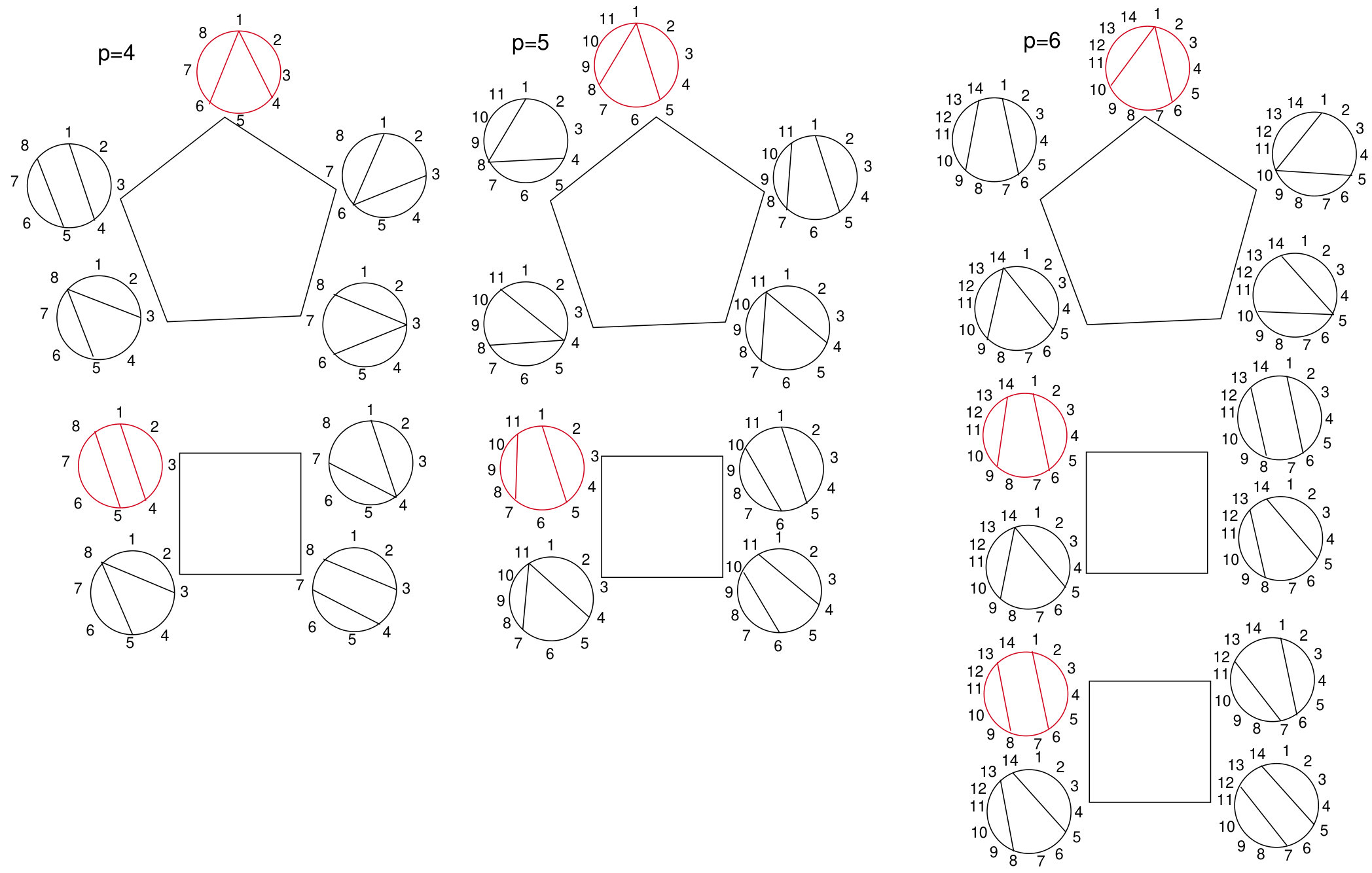 Figure 1
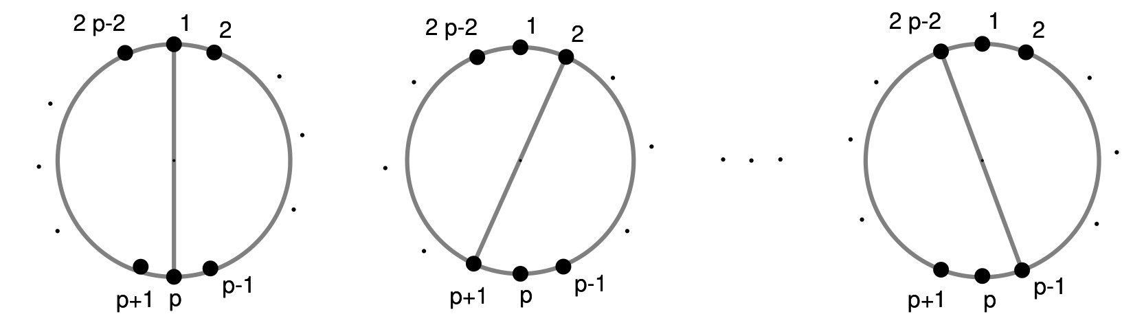 Figure 2
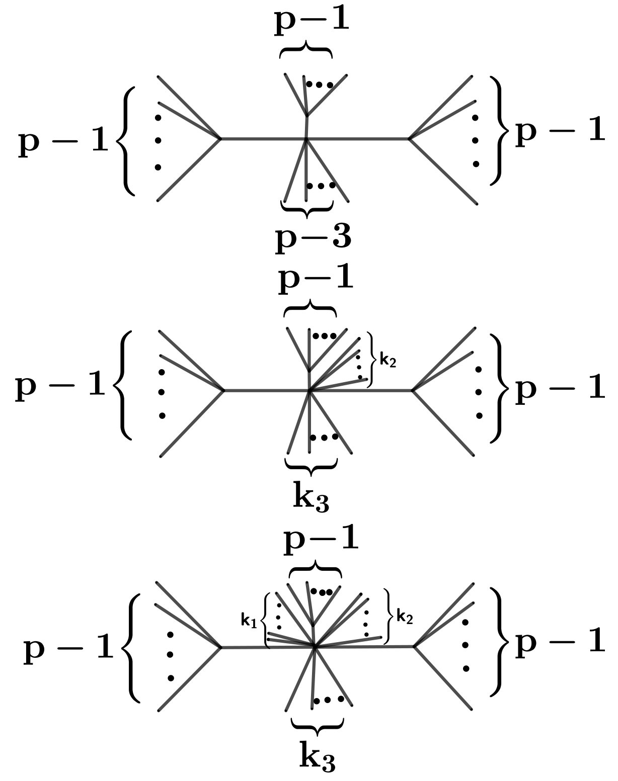 Figure 3
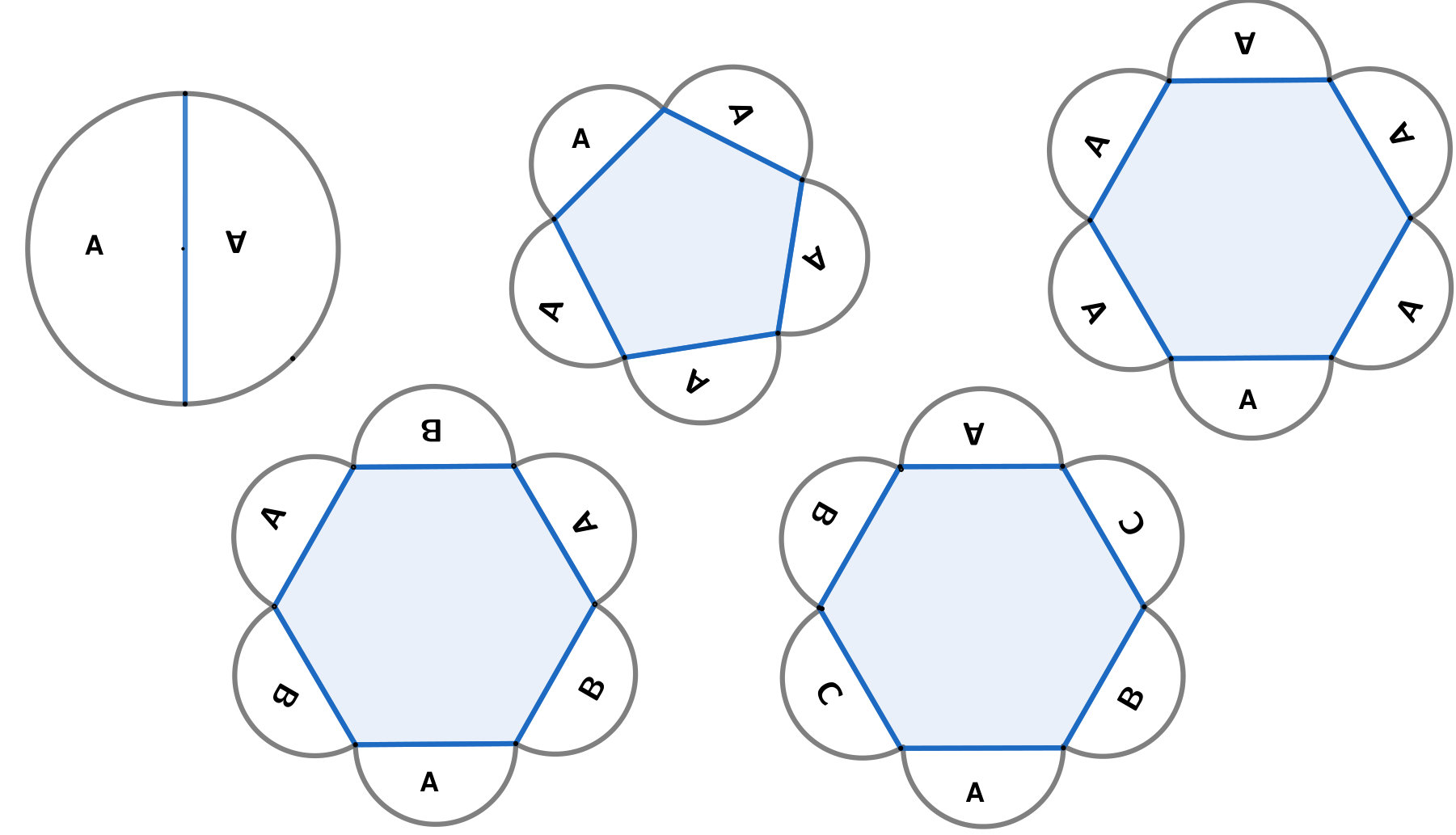 Figure 4
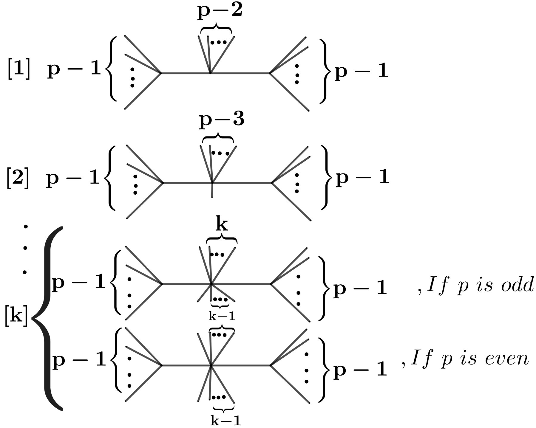 Figure 5
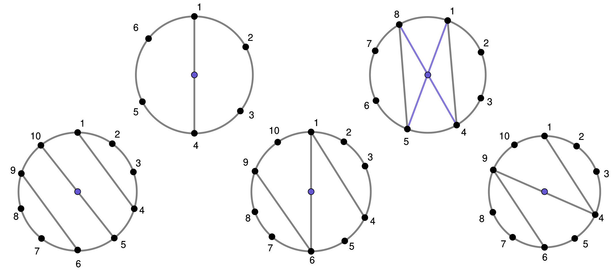 Figure 6
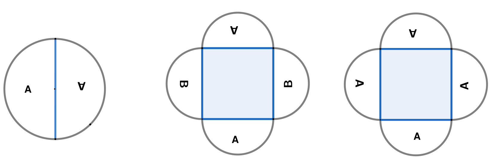 Figure 7
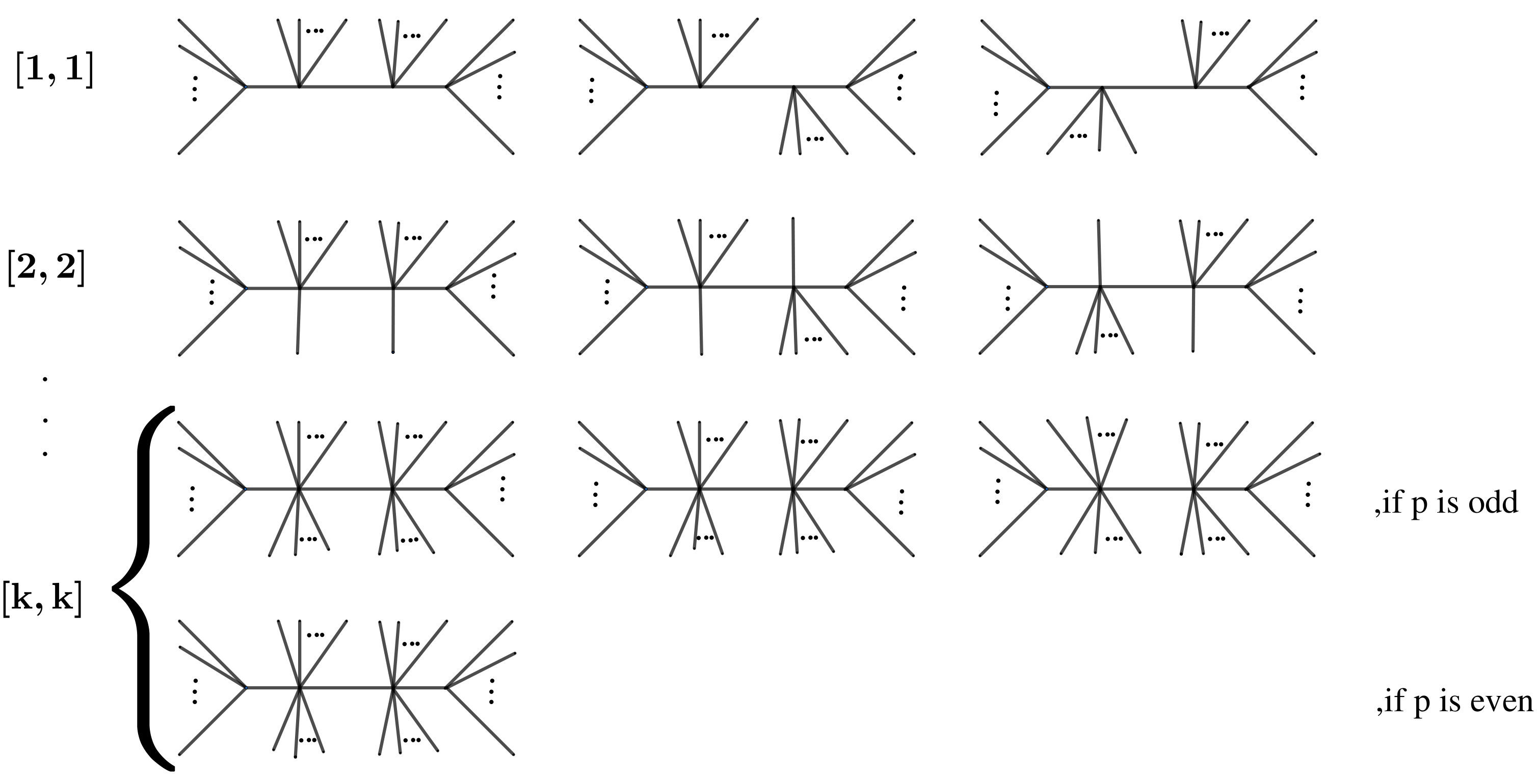 Figure 8
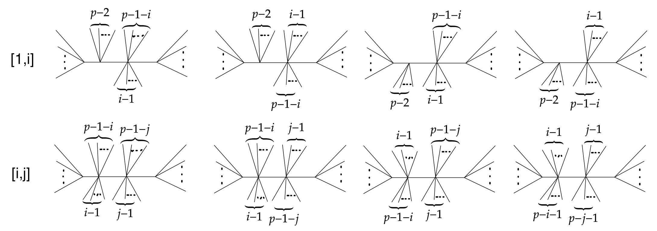 Figure 9
| Type of primitive | number of primitives | period of the primitive |
|---|---|---|
| 3 | 1 with | |
| with | 2 with | |
| 1 , if is even | ||
| 3 , if is odd | 1 with | |
| 2 with | ||
| with | 4 | |
| 2 , if p even | ||
| with | 4 , if p odd |
| Type of primitive | number of primitives | period of the primitive |
|---|---|---|
| 1 | ||
| 1 , if is odd | ||
| 0 , if is even | ||
| , if p is even | ||
| , if p is odd | ||
| , if p is even | ||
| , if p is odd | ||
| , if | ||
| 1 , if | ||
| 0 , otherwise | ||
| , if is even | ||
| , if is odd | ||
| , if |
Peer Reviews
No public reviews on file for this paper yet. If you reviewed it on a platform where reviews are public (OpenReview, ICLR, NeurIPS, ICML), you can paste yours below so the community can read it here.
Videos
No videos yet. Explain this paper in a talk, walkthrough, or lecture? Add one.
The positive geometry for interactions
Prashanth Raman
* Institute of Mathematical Sciences, Taramani, Chennai 600 113, India*
* Homi Bhabha National Institute, Anushakti Nagar, Mumbai 400085, India*
* E-mail : [email protected]*
Abstract
Starting with the seminal work of Arkani-Hamed et al [1], in [2], the “Amplituhedron program” was extended to analyzing (planar) amplitudes in massless theory. In this paper we show that the program can be further extended to include () interactions. We show that tree-level planar amplitudes in these theories can be obtained from geometry of polytopes called accordiohedron which naturally sits inside kinematic space. As in the case of quartic interactions the accordiohedron of a given dimension is not unique, and we show that a weighted sum of residues of the canonical form on these polytopes can be used to compute scattering amplitudes. We finally provide a prescription to compute the weights and demonstrate how it works in various examples.
Contents
1 Introduction
In [1, 3] a space-time independent formulation for scattering amplitudes in SYM was proposed. A key feature of this formulation was that scattering amplitudes were to be thought of as differential forms rather than functions and it was shown that there is a precise connection between an object called the amplituhedron living in an auxiliary space and planar scattering amplitudes in SYM. It was further shown that unitarity and locality emerge quite naturally from geometric properties of the amplituhedron. Understanding scattering amplitudes in terms on canonical form on the amplituhedron makes the dual conformal symmetry manifest and has already produced striking results regarding positivity properties of the amplitudes as well as computational simplification for higher loop amplitudes [4, 5].
Recently Arkani-Hamed et al [1] extended this formulation to non-supersymmetric domain by analysing tree-level amplitudes of bi-adjoint scalar theory. A precise connection was established between a polytope called the associahedron and scattering amplitude of the theory. It was shown that associahedron (which is a combinatorial polytope) can be embedded as a convex polytope in the kinematic space and the canonical form associated to it is the scattering form for theory. It was also shown that various properties like soft limits and recursion relations of scattering amplitudes could be obtained from geometric properties of the associahedron. This formulation was further extended to include 1-loop amplitudes in bi-adjoint theory [6, 7].
A natural question to ask is for what class of theories such a formulation exists. In particular for theories containing independent quartic and higher order vertices, does this picture relating scattering amplitudes to differential forms and convex polytopes continues to hold. First step in this direction was taken in [2] where it was shown that for tree-level planar amplitudes in theory such a formulation does indeed exist. It was established in [2] that there is a relationship between the scattering amplitude, scattering forms and objects called Stokes polytope. There were however important structural differences between the amplituhedron/associahedron picture and the picture that emerged in the case of quartic interactions. Namely, for an -particle scattering, the corresponding geometry was a union of many polytopes of a given dimension and one had to account for all of them to capture complete tree-level planar scattering amplitude.
In this paper, we extend these ideas to all theories by establishing a connection between unique planar scattering forms and convex polytopes called accordiohedron. We also show that (just as in the case of cubic and quartic interactions), geometric realisation of accordiohedron inside the kinematic space leads one to identify scattering amplitudes in such theories with canonical top forms of the accordiohedron.
One of the key motivations for our work (apart from it’s intrinsic interest in developing the Amplituhedron program further) was already outlined in [2] and arises from trying to better understand the CHY formulation for theories [8, 9]. Unlike bi-adjoint scalar field theory, or Yang-Mills theory the CHY integrands associated to theories are not d-log forms and hence do not seem to have a clear geometric meaning in terms of forms on the moduli space. Our hope is that by first understanding the structure of such forms in kinematic space, we may be able to better understand CHY formula for such theories.
The rest of the paper is organised as follows. In section (2) we define the notion Q-Compatibility and use it to define the accordiohedron for interactions. In section (3) we explain how to embed the accordiohedron in kinematic space and how to obtain the scattering amplitude from the accordiohedron by intorducing primitives and weights to simplify our computations. In section(4) we derive a formula for the number of primitves of a given dimension and provide a classification all primitves up to , we also provide general prescription for determining the weights. In section (5) we prove factorization for accordiohedra and also discuss the role of factorisation in determining the weights. We finally end with some conclusions and future directions.
2 Amplitudes and Accordiohedron
We shall begin by defining an object called the accordiohedron [10, 11] associated with general dissections of polygons. We shall then show how this reduces to the associahedron and Stokes polytopes [1, 2] for cubic and quartic interactions respectively. We shall then argue that the accordiohedron is thus the natural candidate for the positive geometry of all interactions with .
2.1 Accordion lattices and Accordiohedra
Let A be a convex polygon. Let us consider the division of A into identical -gons which we call -angulation of A. We can represent A as a set of points on the unit circle oriented clockwise where the arcs represent edges of A and chords represent diagonals of A. The simplest example is the case where we divide -gon A into two -gons (see figure (1)). There are possible -angulations which correspond to having the diagonals .
We define a notion of Q-compatible diagonal as 111In [10, 11] there is different definition of compatability, but these two definitions can be shown to be equivalent to each other and we shall use the definition (1) as its most suited for our purposes. We thank Alok Laddha for explaining this fact to us. :
[TABLE]
We can use this rule to define accordion lattices of dimension associated with a reference -angulation P 222We consider only the case where we divide the polygon into -gons in this paper, but accordion lattices are defined for arbitrary dissections. as follows:
- •
We can start with any -angulation of a convex polygon with diagonals.
- •
In the first step for each of the diagonals, we go to the unique -gon which contains it and replace it with its -compatible diagonal.
- •
In the second step for each of the -angulations at the end of step one we choose one of the original diagonals and replace it with its -compatible diagonal as in step one.
- •
*We repeat this till none of the original diagonals remain in step . *
This generates a graph333More precisely one can define a partial order on the the set of all -angulations that can be obtained from a particular -angulation P, which has a maximal and a minimal element ( itself) thus making it lattice and this procedure generates the Hasse diagram of the lattice which is the 1-skeleton of a convex polytope called the Accordiohedron [10, 11], which we shall also call .444Interestingly enough, there is yet another, “complimentary” family of polytopes known as graph associahedra [12] which also had deep connections with geometry of scattering amplitudes. In contrast to accordiohedron, graph associahedra can not always be obtained by considering dissections of polygons. graph associahedra is a set of polytopes which includes, associahedron, permutahedron, halohedron etc. Many of these members, e.g. permutahedron and halohedron are associated to amplitudes in bi-adjoint scalar theory with non-planar [13] and 1-loop amplitudes [7] respectively. It is intriguing that one class of polytopes helps one to move beyond tree-level and planarity in bi-adjoint theories and the other class helps one move beyond cubic vertices.
[TABLE]
In the case of cubic interactions (), (1) reduces to which is the usual mutation rule and the resulting accordiohedron is the associahedron [1].
In the case of quartic interactions (), (1) reduces to which was the Q compatibility rule defined in [14] and the accordiohedron was shown to be the Stokes polytope [2].
Thus the Accordiohedra are a general class of polytopes which contain both associahedron and Stokes polytopes as special cases when the -angulations corresponds to triangulations and quadrangulations respectively. The accordiohedra with also retains many of the features of the Stokes polytopes we had discussed earlier in [2] including the fact that the accordiohedron of a given dimension is not unique and depends on the reference -angulation P, which is due to the fact that (1) is not an equivalence relation as , but except when .
The case is special in this sense as for is independent of , as every diagonal is -compatible with every other diagonal and thus we could start with any triangulation and we would generate all possible triangulations.
The accordiohedron obtained by starting with a particular -angulation is also completely determined by the relative configuration of diagonals.555From the perspective of Feynman graphs this is equivalent to saying that there is an accordiohedron for each topological class of graphs.
The accordiohedron are lines with vertices and for .
The case the accordiohedron can be either pentagons or squares depending on whether the two diagonals meet or don’t meet respectively (see fig(2)) just as in the case of Stokes polytopes. In other words for all provided both and have the same configuration of diagonals, we shall prove this in a later section (4.3) by establishing the precise maps between vertices of the Stokes polytope and that of the accordiohedron.
The case the accordiohedra continue to be one of the four Stokes polytopes with different multiplicities, i.e., for all provided and have the same configuration of diagonals. We elaborate on this in section (4.4). We expect that at higher new polytopes which are not one of the Stokes polytopes will be eventually generated.
3 Positive geometry for interactions
We would like to show that the accordiohedron is the positive geometry associated to interactions. We shall do this by first embedding the accordiohedron into kinematic space and then showing that the canonical form of the accordiohedron when pulled back gives the right planar scattering amplitude for interactions. We start by noting the following facts:
- •
The only tree level amplitudes consistent with interactions have external legs for vertices.
- •
Analogously to the cubic and quartic cases there is a 1-1 correspondence between planar tree level Feynman graphs and dissections of - gon into p-gons.
- •
We also require the accordiohedron to have dimension , which is the number of propagators.666This is because we require the top-form on the positive geometry, once embedded in kinematic space to produce the right scattering amplitude.
We shall first introduce some notations and variables that we shall use to describe the kinematic space.
3.1 Kinematic space
We shall primarily follow the conventions of [1] which we briefly summarise here.
The kinematic space of massless momenta in dimensions (with ) is spanned by the Mandelstram variables:
[TABLE]
that satisfy momentum conservation
[TABLE]
For any set of particle labels we can define generalised Mandelstram variables as:
[TABLE]
A more convenient basis for the kinematic for our purposes are the planar kinematic variables,
[TABLE]
It is clear that and due to masslessness and momentum conservation respectively. The mandelstram variables can be written interns of planar variables as
[TABLE]
The planar variables can be interpreted as the the length of a diagonal between vertices and of an -gon which has the momenta as sides.
3.2 Planar scattering form for interactions
We would like to define a planar scattering form for interactions. We can associate to each planar graph with propagators a scattering form:
[TABLE]
where, .
Thus, when we sum over all planar graphs we have several possible scattering forms. Since we do not have a notion of *projectivity * except in the case of which helps us fix a unique scattering form [1]. We can choose a particular reference graph (equivalently a -angulation ) and look at only those subset of graphs which are related to this graph by a sequence of -flips namely all the vertices of the accordiohedron. If a graph is related to by an odd (even) number of -flips we can associate sign to it. Thus, we can define a -angulation dependent planar scattering form :
[TABLE]
Since, the -compatible -angulations corresponding to any reference -angulation does not exhaust all the -angulations, we need to define such a planar scattering form for each .
In the case the set of -compatible p-angulations are 777Here the signs denote , when we have multiple diagonals we need to carefully maintain the order of diagonals when we flip as it contibutes to the sign. the planar scattering forms for which are:
[TABLE]
where, modulo with .
We now turn to embedding the accordiohedron in kinematic space and showing that when the planar scattering form is pulled back onto the accordiohedron it gives the canonical form of the accordiohedron.
3.3 Locating the accordiohedron inside kinematic space
We now define the kinematic accordiohedron . We locate the accordiohedron inside the positive region of kinematic space for all by imposing the following constraints:
[TABLE]
where are positive constants.888In the case when that is when the Accordiohedron is a Stokes polytope, there is a canonical choice for the additional constraints if the Stokes polytope is itself not an Associahedron [2]. However for we do not have any canonical choice of these constraints. As we show in this section, there is at least one choice which consistently embeds the Accordiohedron in the Kinematic space.
Physically we choose the above set of constraints as they do not appear as propagators of any graph. The first constraint above is the famous associahedron embedding [1]. We have thus embedded the accordiohedron inside the associahedron. The positivity of ’s, the above constraints along with the equation (2) are a set of inequalities satisfied by the which makes the convexity of the accodiohedron manifest.
We first consider the case with the reference -angulation to be for . For we can choose to be and respectively. The above constraints then translate to:
p=5: which a line with boundaries at
provided the following are satisfied 999Since we are slicing the associahedron using some hyperplanes to get the accordiohedron these constraints tell us how the slicing should be made. For higher we shall not state these constraints for brevity but we shall assume that they are satisfied.
p=6: which a line with boundaries at
provided the following are satisfied
[TABLE]
The above equations define lines with -compatible vertices and for and respectively. We can trivially repeat this exercise for any other reference p-angulation , the results of which can be obtained by taking in the above equations. We can now pull back the scattering form onto the accordiohedron as:
[TABLE]
with .
As before to get the full amplitude we consider a weighted sum of over all .
[TABLE]
It is clear that if and only if for all .
Thus, we can simplify our computation by considering a subset of -angulations called primitive -angulations for which:
(a) no two members of the set are related to each other by cyclic permutations and
(b) all the other -angulations can be obtained by a (sequence of) cyclic permutations of one of the s belonging to the set.
The primitives are the class of rotationally inequivalent diagrams. Since, a rotation does not change the relative configuration of diagonals it is clear that accodiohedra remain the same for all the diagrams that belong to a primitive class and that the weights depend only on primitives. We shall say more about primitives in section (4).
[TABLE]
For now let us look at a couple of examples to see how finding primitive accordiohedra and their weights help us in getting the scattering amplitude.
In the case above there was only one primitive .
We consider the case for for which we now have the set of primitives as (see figure(2)) and respectively. The set of -compatible -angulations for these are:
[TABLE]
The embedding constraints (3.3) can be solved to obtain:
p=5: For P=(15,711), with to be
[TABLE]
The positivity of carves out a square region in the space. The accordiohedron in this case is also a square as we had emphasised in section (2.1).
For P=(15,18), with to be
[TABLE]
p=6: For P=(16,914), with to be
[TABLE]
For P=(16,813), with to be
[TABLE]
For P=(16,110), with to be
[TABLE]
When pulled back onto constraints the corresponding ’s are:
:
[TABLE]
Plugging the above forms into eq. (5) with weights , (see section (4.5) for details) gives the right amplitude.
:
[TABLE]
Plugging the above forms into equation (5) with weights , , (see section (4.5) for details) gives the right amplitude.
4 Analysing the combinatorics of Accordiohedra
Both in [2] and in the present case, a complete computation of the amplitude from the geometry of the polytope requires determination of all the primitives of a given dimension and computation of the corresponding weights. We shall address the problem in this section. We emphasise that this a purely combinatorial problem and hence does not depend on the construction of kinematic space accordiohedron. In sections (4.1) ,(4.2) we shall first derive formulae to count the number of primitive accordiohedra of a given dimension . Then in sections (4.3) ,(4.4) we provide a complete classification of primitive accordiohedra for and compute the corresponding weights for any interactions. Let us first consider the quartic case.
4.1 Counting primitives for the quartic case
In this section we shall address the quartic case first and provide a formula for the number of primitive Stokes polytopes of a given dimension . The main result of this section is:
[TABLE]
We shall now prove this result.
We shall consider a -gon as equally spaced points on the circle i.e. with . The edges of the polygon correspond to arcs on the circle and the diagonals of a quadrangulation correspond to chords.
There is a natural action of the dihedral group on any given quadrangulation which is generated by rotation and reflections about a given diagonal. We are interested in counting primitive quadrangulations, no two of which are related to each other by a cyclic permutation, which corresponds to a rotation on the circle. Thus, it is sufficient to consider only the cyclic group for our purposes. The problem of counting primitive quadrangulations is thus equivalent to finding the number orbits of the set of all quadrangulations of a -gon under the action of the cyclic group .
We shall do this by using the celebrated Burnside’s lemma, which is the standard way to count the number of orbits for the action of any finite group on a set . It states that the number of orbits is equal to the average number of points that remain invariant when acted on by elements of .
[TABLE]
Thus, to count the number of primitive quadrangulations we just need to find the subset of quadrangulations that are invariant under some rotation. This problem has been addressed by [15] using the method of generating functions, but we shall take a simpler approach here following [16].
We can consider the division of -gon into quadrilaterals. We first note that the centre of the circle is left invariant by the action of the cyclic group . The centre of the circle can lie on:
(1) A diameter. This can only happen when is odd since, the relative angle between the end points of this diameter has to .
(2) The midpoint of an invariant cell i.e. on the point of intersection of the diagonals of a centre square which remains invariant.
In case (1) the diameter forms an axis of symmetry and has to be left invariant by rotations and it is clear that the only possible rotation which does this is by and the quadrangulation consists of a left and a right part where the left part is a rotation of the right one.( see figure(3) ).
In case (2) the diagonals can either be rotated to themselves or into each other. This can only be accomplished by rotations of and the corresponding quadrangulations are shown in the figure (3).
The number of quadrangualtions of -gon into quadrangles is given by the Fuss-Catalan number (which we derive in appendix A). The number of quadrangulations of type (1) is , as we can choose a diameter in ways and for each choice of the diameter there sub-quadrangulations .
The number of quadrantulations of type (2) depends on whether is divisible by 2 or 4 and is given by and respectively. In the case where we can divide into which we call and in the third figure of (3) and the number of such quadrangulations would correspond to and respectively. The total number of such quadrangulations would then be and since there are ways we can relabel the invariant square. Using the following combinatorial identity (see appendix B).
[TABLE]
We have invariant quadrangulations under a rotation by .
When we have subquadrangulations as shown in figure (3). There are also ways to relabel the invariant cell and thus there are a total of quadrangulations that are invariant under a rotation by . Thus, after also including the identity rotation which leaves all the elements invariant we get the total number of primitive quadrangulations is given by:
[TABLE]
We can easily check the above formula for cases by using and for . The set of invariant quadrangulations is shown in the figure (4) below.
n=1: We have 3 quadrangulations which remain invariant under rotation by .
[TABLE]
n=2: There are 4 quadrangulations with which remain invariant under rotation by .
[TABLE]
n=3: There are 15 quadrangulations with
[TABLE]
4.2 counting primitives for case
We shall now extend our analysis for the quartic case to any general and provide a formula for the number of primitive accordiohedra of dimension . The number of primitives p-angulations of an -gon is the same as the number of orbits of the cyclic group when it acts on the set of all p-angulations. There number of such orbits can be straightforwardly computed from Burnside’s lemma just as we had done in (4.1). We proceed analogously to the quartic case (4.1) by noting that the centre of the circle is invariant under any rotation and can lie:
(1) On a diameter, this happens only when is odd and leaves the -angulation invariant under a rotation by (see figure (5)).
(2) Inside an invariant cell, in this case we have -angulations for every which is invariant under rotation by (see figure (5) ).
The total number of -angulations of an -gon into -gons is given by the Fuss Catalan number (see appendix A for a proof of this).
In case (1) there are choices for the diameter and choices for . Thus, there are a total of invariant -angulations under a rotation by .
In case (2) there is an invariant cell and the remaining cells can be divided into parts for every in , ,… ways s.t. which we call , , etc. For each such there are -angulations which remain invariant under a rotation, where is the Euler totient function which counts positive integers up to which are relatively prime to it.
For if is the prime factorisation of then is given by:
[TABLE]
Thus, the total number of such -angulations once we also include identity rotation is:
[TABLE]
where, we have used the combinatorial identity
[TABLE]
with which we shall prove in appendix B.
To determine the weights we would need to actually identify the primitive accordiohedra, then we need to find all the vertices of the accordiohedra starting with these primitives as the reference -angulations. There is no general classification for primitives of an arbitrary dimension to our knowledge since they grow as . We provide a complete classification for and give the compute the corresponding weights.
4.3 primitives and weights for case
We would like to provide the details of the primitives and weights for interactions for the ( 2d case). In this case there are 3 vertices with legs. We could try to recursively construct these graphs from the graphs. So without loss of generality we consider only Feynman graphs in which two of the vertices lie in a line as shown in the figure(6). The 3rd vertex can then be made to lie on the central line connecting the first two vertices and it can be either above or below this line. These graphs can be denoted as such that , where the 3rd vertex has legs above and legs below the central line.
Since, we are only interested in primitives the graphs for which 3rd vertices are and correspond to the same primitive graph. Thus, without loss of generality we can choose the diagrams in which the 3rd vertex has more legs above the central vertex than below it to be primitive graphs namely , ,…, . We shall call them ,,…,, where .
The primitives are all shown in the above figure(6). We shall now show that these are the only primitives. It is clear that all the graphs above are inequivalent under cyclic permutations. As explained earlier the total number of such graphs is given by the Fuss-Catalan number
[TABLE]
We shall show that if we perform the channel sum starting with these primitives we generate all the graphs. A cyclic permutation corresponds to a clockwise rotation of the labels and every graph returns to itself after a rotation of period but a graph for which the 3rd vertex is symmetric about the central line returns to itself after only half a rotation i.e has a period . The only such graph is the last graph in the case when . Thus, the total number of graphs generated by performing sum over all the channels is :
[TABLE]
using
[TABLE]
we get the total number of graphs to be which agrees with our results from (4.2). As explained in the previous subsection the accordiohedra generated by starting with a particular graph (or p-angulation ) depends only on the relative configuration of the diagonals and in this case since there are 2 diagonals the only possibilities are:
The diagonals meet as in , in this case the accordiohedron is an associahedron .(see (2)) 2. 2.
The diagonals do not meet as in ,… ,, in all these other cases the accordiohedron turns out to be a square.
We can provide a mapping between the vertices of the Stokes polytope and for the case as follows:
When the two diagonals meet then with and we could map the vertices of the Stokes polytope which is a pentagon in case with the pentagon corresponding to the accordiohedra once we notice that the all which is part of some diagonal do not appear in a vertex of the Stokes polytope. For example in the case of only appear and similarly in the case of the accordiohedron exactly 6 out of a possible appear thus we could trivially define a map between the two as follows:
[TABLE] 2. 2.
When the two diagonals do not meet then we notice that there are several possible choices of the diagonals for , but we notice that the maximum number of ’s which can appear for any choice of is 8, since each diagonal appears twice thus there are only 4 possible ’s. We can thus identify these ’s with and define a mapping.
For example we provide such a mapping between the Stokes polytope corresponding to and the accordiohedra corresponding to (see (2) )below:
p=5: With
[TABLE]
p=6: With
[TABLE]
It is straightforward to find such a mapping for general and a general choice of . 101010It is a well known fact that there is a unique 2d convex polytope with a given number of vertices, so the above mapping is not really needed here but in the case of 3 and higher dimensional polytopes ,there could be several polytopes with same -vector, thus we would need such a mapping to be sure that the polytopes are isomorphic.
4.4 primitives for case
We would now try to find all primitive graphs for the case. In this case there are 4 vertices with legs. As before we can try to recursively construct primitive graphs from case.
There are two possible ways we add the 4th vertex which could be any of the types in the case :
We can add another central vertex either above or below the central line to a graph. We call these graphs and . ( see figures (7), (9)). 2. 2.
We can add the vertex to any one of the external legs of the 3rd vertex. We denote these graphs by , where .
There are 3 primitives of the type for each since the graphs where both vertices are down are just cyclic permutations of the graph with both vertices up. In case where is even you also have a vertex with equal number of legs above and below the central line, thus there is only one such primitive corresponding to this case. The graphs with one central vertex up and the other down (the 2nd and 3rd graphs for each ) have half periods i.e. under cyclic permutations they go back to themselves after operations. The same is also true for the symmetric vertex when is even. All other graphs have full period of .
There are 4 primitives for each since now the graphs with both vertices down are inequivalent to the ones with both vertices up under cyclic permutations. When is even we have only 2 primitives of the type since is symmetric. All these graphs all have a period of .
These possibilities are summarised in the table 1 below:
We could also consider graphs of the type such that . Since there are non zero solutions of , in this case we have the following possibilities:
- •
We have a graph of the type (0,0,p-3) with period .
- •
We can have a two graphs and for each with (which are inequivalent since they are reflections of each other) and when is odd we also have one graph with with period . Thus, there are
[TABLE]
such diagrams.
- •
We have one graph for each with with period . In this case we have
[TABLE]
such diagrams.
- •
When we have exactly one graph with which has a period .
- •
We have two graphs and for each . In this case we have
[TABLE]
These possibilities are summarised in the table 2 below.
We can now find the total number of -angulations by summing over all channels by multiplying columns two and three of the tables above and adding them up.
[TABLE]
The result of this exercise turns out to be which matches with the expected Fuss-Catalan number which agrees with equation (4.2)
[TABLE]
Since there are 3 diagonals now the relative configuration of diagonals can be of one of the following types:
None of the diagonals meet - in this case the corresponding accordiohedron is a cube. There are graphs of this type namely , with and with . 2. 2.
Two of the diagonals meet - in this case the corresponding accordiohedron is of the mixed type. There are graphs of this type namely with and with . 3. 3.
All three diagonals meet at a vertex or form zig-zag configuration in this case the corresponding accordiohedron is an associahedron. There are graphs of this type namely . 4. 4.
All three diagonals meet and form an inverted U configuration in this case the corresponding accordiohedron is of the Lucas type. There is exactly one graph of this type which is .
Thus the total number of primitives is :
[TABLE]
which agrees with we our general formula (4.2).
The accordiohedra for we get continue to be one of the four kinds of Stokes polytopes. We could define a function from vertices of the Stokes polytopes to that of the accordiohedra as we had done in the case to establish that this is indeed the case. We can thus continue to use the same names Lucas, Mixed etc for the Stokes polytopes for accordiohedra as well. We expect that at sufficiently higher , accordiohedra will be generated which do not correspond to any Stokes polytope.
4.5 Determination of the weights
In this section we shall provide a simple method to determine the weights for the general case and demonstrate the method in a few examples. We recall that we had the reduced amplitude which is a weighted sum of canonical forms of all the primitive accordiohedra of a given dimension . We would like to determine the weights such that this gives the full amplitude i.e. .
The full amplitude is given by :
[TABLE]
where, the sum is over all that form a complete -angulation.
Thus, to get the full amplitude from the partial amplitude we need to impose the constraint that each appears exactly once.
But as we had emphasised before the accordiohedron depends only on the relative configuration of diagonals of the reference -angulation which does not change under rotations and thus it is sufficient to impose these constraints for the primitive -angulations.
[TABLE]
where, is number of times primitive appears in the vertices of all accodiohedra, are the corresponding weights.
Since, we have managed to classify all the primitives unto we should be able to implement this straightforward procedure to get all the weights and we shall now discuss our results.
We shall first see what these conditions are for in the cases.
: In this case there are two primitives as we had explained in the section (4.3) and we get:
[TABLE]
which can be solved to give:
,
: In this case there are 3 primitives and we get:
[TABLE]
which can be solved to give:
,
We can similarly do this for any with and the results are the following :
For
[TABLE]
and For
[TABLE]
with .
The ’s for case with are given below (for the sake of brevity we shall call ’s corresponding to as ): If is even then :
; ; ; ; …
; ,
If is odd then the results for the first few cases are : p=5 : with ; ; ; .
p=7 : with ; , with ; ; ,
; ; .
p=9 : with ; , with ; , with ; ; ; ; ; ,
; ; .
p=11: with ; , with ;
, with ; , with ; ; ;
; ; ; ; ;
; ; ; .
5 Factorization
One of the remarkable consequences of relating tree level scattering amplitudes to positive geometries like associahedron, Stokes polytope is the fact that geometric factorization implied physical factorization of scattering amplitude. This in turn implied that tree-level unitarity and locality are emergent properties of the positive geometry [1, 2]. In this section we will try to argue that this is indeed the case even for planar amplitudes in massless theory. We shall first argue that the geometric factorisation of accordiohedron holds and then show how this leads to the factorisation of the amplitude.
In [2] it was shown how the factorization of Stokes polytope leads to a recursions relation on ’s. We shall see that even for more general Accordiohedra ’s are required to satisfy analogous recursion relations.
Our first assertion is the following. Given any diagonal , consider all which contains and the consider all the corresponding kinematic accordiohedron . We contend that for each accordiohedron, the corresponding facet is a product of lower dimensional accordiohedra.
[TABLE]
where and are such that .
is the -angulation of the polygon and is the -angulation of . Now we know that, on any planar scattering variable is a linear combination of and remaining ’s which constitute . Hence in order to prove this assertion we need to show that any with can be written as a linear combination of and elements of and similarly any variable in the complimentary set can be written in terms of and elements of .
However this is immediate since we know from the factorization property of associahedron proven in [1] that any , some of these and the others are constrained via . This proves our assertion. Thus facet factorizes into two lower dimensional accordiohedra.
Our second assertion is that the geometric factorization implies amplitude factorization of theory. This assertion is based on the following two facts (For details, we refer the reader to appendix A of [1] and [4]). (1) As the accordiohedra is a positive geometry, we know that it’s canonical form satisfies the following properties satisfed by canonical form on any positive geometry
[TABLE]
where we think of as defined on the embedding space and is any subspace in the embedding space which contains the face . (2) It is also known that if then
[TABLE]
Thus we immediately see that
[TABLE]
where .
We thus see that residue over each accordiohedron which contains a boundary factorizes into residues over lower dimensional accordiohedra. This factorization property naturally implies factorization of amplitudes as follows. Consider the -gon with a diagonal (with such that this diagonal can be part of a -angulation). This diagonal subdivides the -gon into a two polygons with vertices and respectively. By considering all the kinematic accordiohedra associated to these polygons, we can evaluate which correspond to left and right sub-amplitudes respectively. This immediately implies that
[TABLE]
This proves physical factorization. We also note that, eqns. (9) and (13) imply following constraints on ’s.
[TABLE]
The left hand side of the above equation involves sum over all accordiohedra for which and the right hand side involves sum over and which range over all the -angulations of the two polygons to the left and right of the diagonal respectively.
It can be verified that in all the examples up to and the ’s do indeed satisfy these constraints.
For there is only one diagonal which we can to be . The accordiohedra is always a line as we had emphasised in section (3.3) and appears in the vertex of exactly two of these lattices namely and . There is only way to divide into and and both these are trivial have . Thus, the above equation (14) gives :
[TABLE]
We could expect that the set of equations (14) would help in determining all the weights [2]. But, as we shall now show this is not the case as (14) provides too few equations. In other words the set of equations (14) provide a set of necessary but not sufficient conditions.
Let, us consider the case for and the diagonal , in this case the -gon gets divided into a -gon and -gon and we have weights and . There are exactly squares and pentagons which contain the diagonal in their vertices. Thus, we have
[TABLE]
We can check that for any other choice of diagonal we get the same equation. It is clear that this is not sufficient to solve for . The solution we had obtained using our prescription in section (4.5) namely does indeed satisfy (15).
6 Conclusions and Future work
Re-formulating scattering amplitudes as differential forms on positive geometries (succinctly called the Amplituhedron program) has had profound impact on how we understand Quantum field theories and how properties like unitarity and locality are a natural consequence of the positive geometries. In theories like Super Yang Mills theory, the Amplituhedron program offers conceptual as well as striking technical advancements in the understanding of planar S-matrix. In the non super-symmetric world, these ideas were extended to bi-adjoint scalar theory in [1] where it was shown that the corresponding amplituhedron is an associahedron in Kinematic space and the canonical form on this associahedron was proportional to the scattering amplitude.
These ideas were extended from cubic to quartic interactions in [2] where the underlying positive geometry was Stokes polytope. However unlike Associahedron, which is unique (in a given dimension), there are several Stokes polytopes in any given dimension and it was shown that one had to sum over canonical forms of all such polytopes to obtain scattering amplitude of theory. Not all Stokes polytopes contributed equally but one had to assign different weights to each Stokes polytope. In [2] it was argued that these weights were not assigned to a given Stokes polytope but to an equivalence class of such polytopes which were related to each other by cyclic permutations and that in each such class, one could choose a representative that we called primitive. Whence the computation of scattering amplitude reduced to the problem of finding all the primitives and assigning weights to them.
In this paper, continuing along the lines of [1, 2] we extend the Amplituhedron program to (tree-level) planar amplitudes for massless scalar field theories with interactions. We have shown that the positive geometry underlying scattering amplitudes in this theory is a class of polytopes called accordiohedron. Accordiahedron is a family of polytopes whose members include associahedron and Stokes Polytope.111111Our work thus shows that the positive geometry underlying planar amplitudes in any scalar field theory is an Accordioheron
Just as in the case of quartic interactions there exists no single accordiohedron of a given dimension and a weighted sum of canonical forms of all the accordiohedra of a given dimension does indeed produce the full planar amplitude. This re-affirms and generalises the result we had obtained in in the case of quartic interactions.
In [2] the problem of counting all primitives (corresponding to Stokes polytopes) of a given dimension had remained open. In this paper we fill this gap and in fact extend this notion to primitive accordioheron. We give an enumeration of the number of primitives at arbitrary dimension and a complete classification of primitive diagrams for .
We then gave a prescription to compute the weights and provided the results for the weights obtained by using our prescription for all in dimensions and for .
Accordioheron is a very general polytope and one may wonder if they can be used to extend the Amplituhedron program to Scalar theories with mixed-vertices (e.g. theories with cubic as well as quartic interactions). It turns out that this is indeed the case. [17]
There are several outstanding questions that arise out of our analysis. In [6] it was shown that the 1-loop integrand of theory also corresponds to canonical form on a polytope which is well known in mathematical literature called Halohedron. Whether this idea can be extended to 1-loop integrand of theories remains to be seen.
One of the most striking results obtained in [1] was the derivation of CHY formula for bi-adjoint scalar interactions from the canonical form on kinematic space associahedron. More in detail, it was shown that the (tree-level) moduli space of CHY scattering equations admits a compactification which is nothing but an Associahedron (called worldsheet Associahedron) and the Scattering equations can be understood as diffeomorphisms between the world-sheet Associahedron and the Associahedron in Kinematic space. It was also shown that the canonical form on Kinematic space Associahedron is nothing but a push-forward of the so-called Park Taylor form which is the canonical form on world-sheet associahedron. Although CHY integrands exist for interactions for they do not admit any such geometric interactions. Our hope is that understanding of kinematic space Accordiohedron is the first step in “geometrizing" the CHY formula for theories.
Acknowledgements
I would like to thank Alok Laddha for many illuminating discussions, constant guidance and various valuable comments on improving the manuscript. I would also like to thank Nemani Suyanaryana, Sujay Ashok, Nima-Arkani Hamed, Song He and Guilio Salvatori and Pinaki Banerjee for insightful discussions and constant encouragement. I would also like to thank the participants of Soft Holography conference in pune and the string group at university of Torino where a preliminary version of this work was presented.
Appendix A Counting planar diagrams
In this appendix we want to derive an explicit formula for the number of planar tree level Feynman diagrams with vertices and arbitrary interactions. We begin by considering the “toy" equations of motion which are equations of motion with a source where we set the d’Alembertian and couplings to one [18]. In other words this is equivalent to setting all propagators and vertices to one. Since, the perturbative solutions to equations of motion with a source are in 1-1 correspondence with connected tree amplitudes, the solutions of these equations gives us the generating functional for the number of Feynman diagrams. Planar diagrams in theory: The toy equations for this case are
[TABLE]
We want to from above which would be the generating function of Planar diagrams. Note that we have instead of since we only want to count planar diagrams which correspond to diagrams that have a fixed ordering. We can invert (16) by treating it as a formal power series and using the Lagrange series inversion formula.
If which is analytic about and then in the neighbourhood of with given by the power series:
[TABLE]
where,
[TABLE]
Using this for (16) with we get
[TABLE]
The number of planar trees with vertices is the coefficient of in the series above which is the Fuss-Catalan number .
Appendix B Proof of identity for Fuss-Catalan numbers
In this appendix we want to prove the identity (8) which we had used in the sections on counting primitives. We begin by noting that if:
[TABLE]
Then we could recursively prove the general identity for example,
[TABLE]
Thus, we shall only need to show (18), and substitute to get (8). We begin with the right hand side of (18)
[TABLE]
To evaluate this expression we shall use,
[TABLE]
We can rearrange (19) as
[TABLE]
We can now apply (20) to each term in the above sum
[TABLE]
[TABLE]
We have replaced the finite sum by an infinite sum since
[TABLE]
vanishes for .
[TABLE]
The only pole in is at , assuming and thus by performing the z integral we get:
[TABLE]
where, we used the fact that the residue of at is given by
Similarly, we have
[TABLE]
Substituting into (21) we get
[TABLE]
The reference list from the paper itself. Each links out to its DOI / PubMed record.
- 1[1] N. Arkani-Hamed, Y. Bai, S. He, and G. Yan, “Scattering Forms and the Positive Geometry of Kinematics, Color and the Worldsheet,” JHEP 05 (2018) 096 , ar Xiv:1711.09102 [hep-th] . · doi ↗
- 2[2] P. Banerjee, A. Laddha, and P. Raman, “Stokes Polytopes : The positive geometry for ϕ 4 superscript italic-ϕ 4 \phi^{4} interactions,” ar Xiv:1811.05904 [hep-th] .
- 3[3] N. Arkani-Hamed and J. Trnka, “The Amplituhedron,” JHEP 10 (2014) 030 , ar Xiv:1312.2007 [hep-th] . · doi ↗
- 4[4] N. Arkani-Hamed, Y. Bai, and T. Lam, “Positive Geometries and Canonical Forms,” JHEP 11 (2017) 039 , ar Xiv:1703.04541 [hep-th] . · doi ↗
- 5[5] N. Arkani-Hamed, C. Langer, A. Yelleshpur Srikant, and J. Trnka, “Deep Into the Amplituhedron: Amplitude Singularities at All Loops and Legs,” Phys. Rev. Lett. 122 no. 5, (2019) 051601 , ar Xiv:1810.08208 [hep-th] . · doi ↗
- 6[6] G. Salvatori and S. L. Cacciatori, “Hyperbolic Geometry and Amplituhedra in 1+2 dimensions,” JHEP 08 (2018) 167 , ar Xiv:1803.05809 [hep-th] . · doi ↗
- 7[7] G. Salvatori, “1-loop Amplitudes from the Halohedron,” ar Xiv:1806.01842 [hep-th] .
- 8[8] F. Cachazo, S. He, and E. Y. Yuan, “Scattering of Massless Particles in Arbitrary Dimensions,” Phys. Rev. Lett. 113 no. 17, (2014) 171601 , ar Xiv:1307.2199 [hep-th] . · doi ↗