A roundabout model with on-ramp queues: exact results and scaling approximations
Jaap Storm, Sandjai Bhulai, Wouter Kager, Michel Mandjes

TL;DR
This paper models a single-lane roundabout with on-ramp queues using a Markovian lattice framework, providing exact stationary distributions and scalable Gaussian and Poisson approximations for traffic performance metrics.
Contribution
It introduces a detailed Markovian model of roundabout traffic dynamics and derives explicit stationary distributions along with novel scaling approximations for large systems.
Findings
Explicit stationary distribution for each cell on the lattice.
Scaling limits approximating joint distributions of segments as Gaussian and Poisson.
A new empirical method to assess convergence in distribution.
Abstract
This paper introduces a general model of a single-lane roundabout, represented as a circular lattice that consists of cells, with Markovian traffic dynamics. Vehicles enter the roundabout via on-ramp queues that have stochastic arrival processes, remain on the roundabout a random number of cells, and depart via off-ramps. Importantly, the model does not oversimplify the dynamics of traffic on roundabouts, while various performance-related quantities (such as delay and queue length) allow an analytical characterization. In particular, we present an explicit expression for the marginal stationary distribution of each cell on the lattice. Moreover, we derive results that give insight on the dependencies between parts of the roundabout, and on the queue distribution. Finally, we find scaling limits that allow, for every partition of the roundabout in segments, to approximate 1) the…
Click any figure to enlarge with its caption.
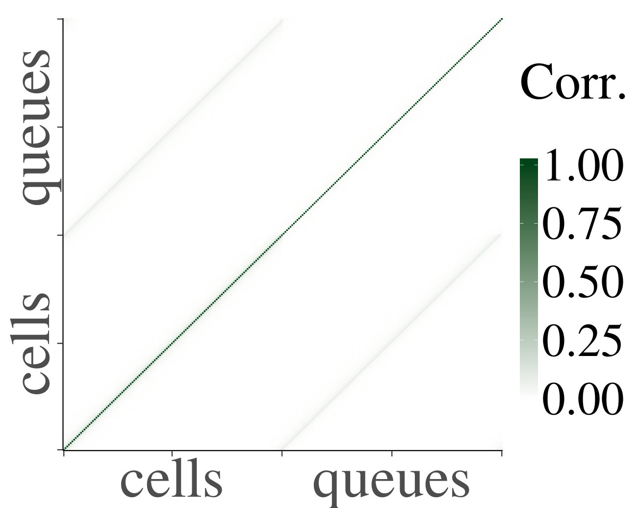 Figure 1
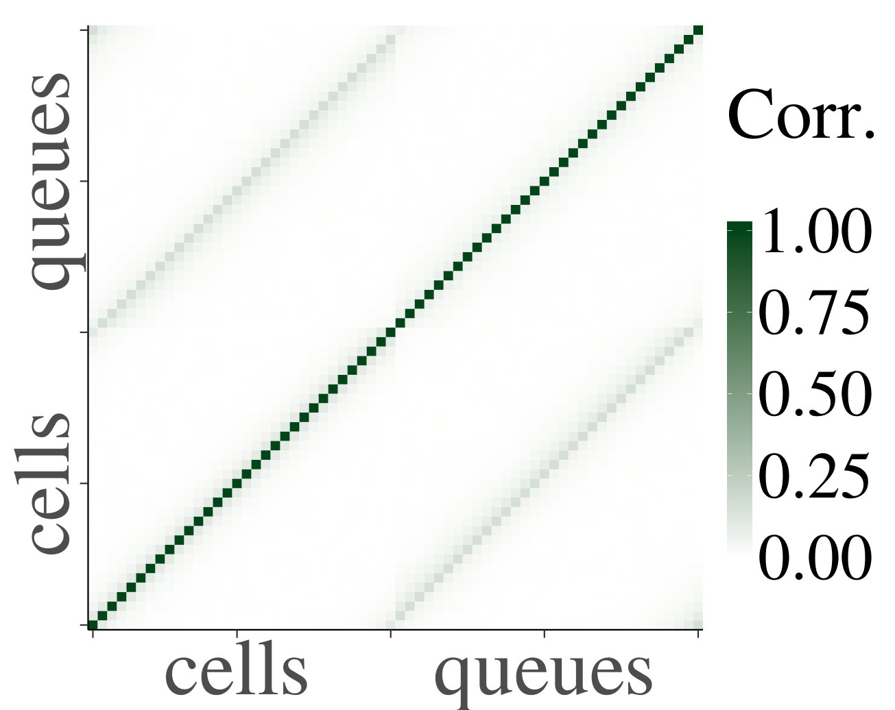 Figure 2
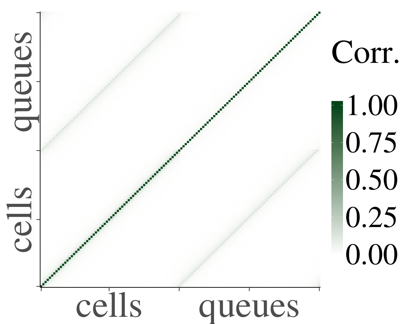 Figure 3
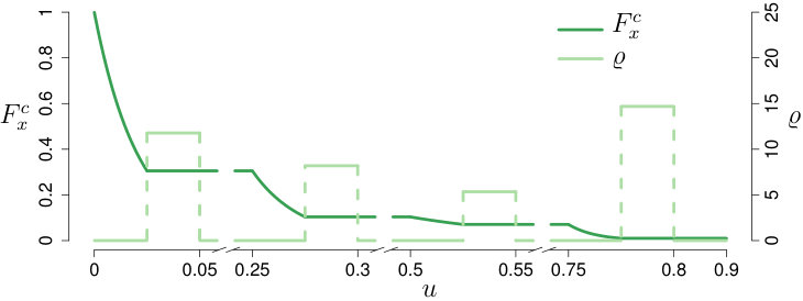 Figure 4
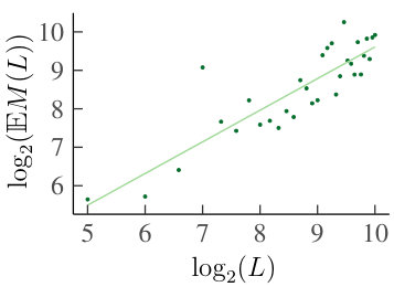 Figure 5
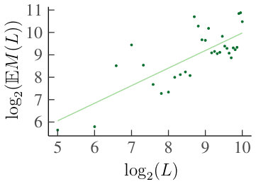 Figure 6
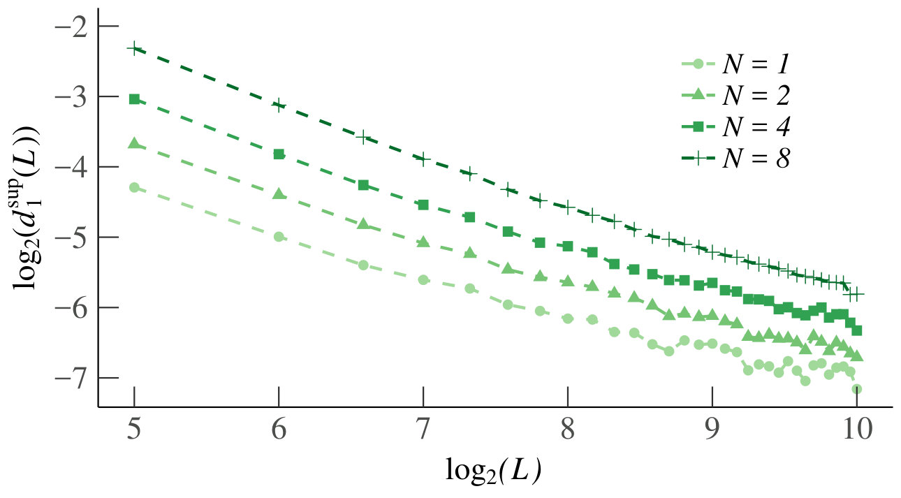 Figure 7
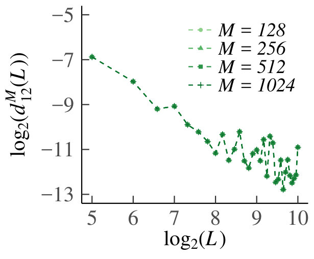 Figure 8
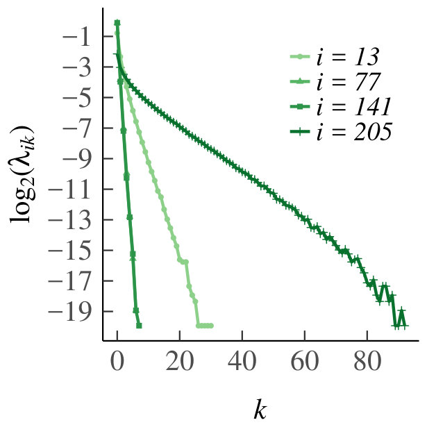 Figure 9
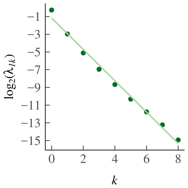 Figure 10
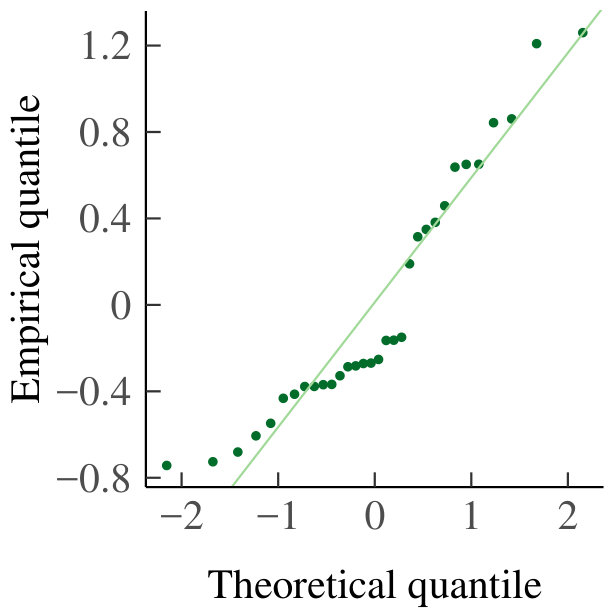 Figure 11
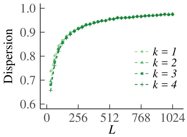 Figure 12
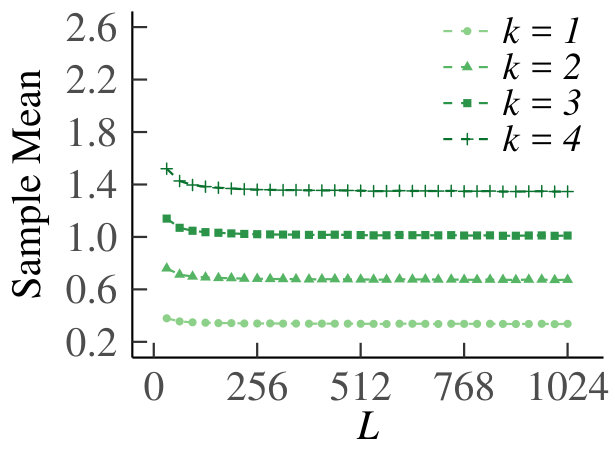 Figure 13
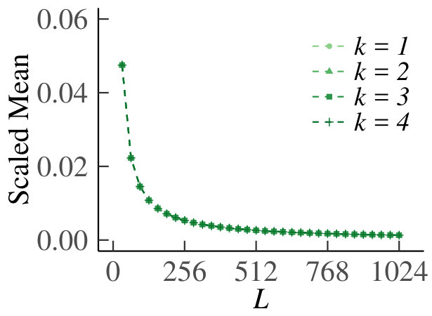 Figure 14
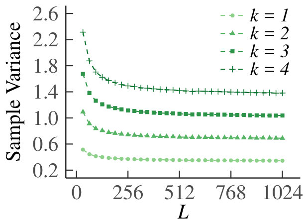 Figure 15
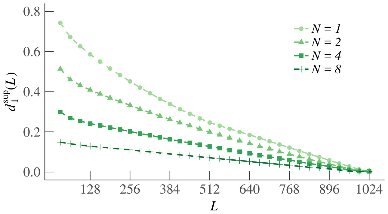 Figure 16
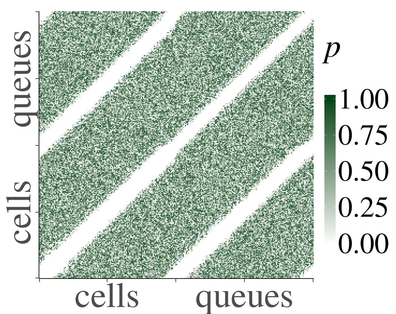 Figure 17
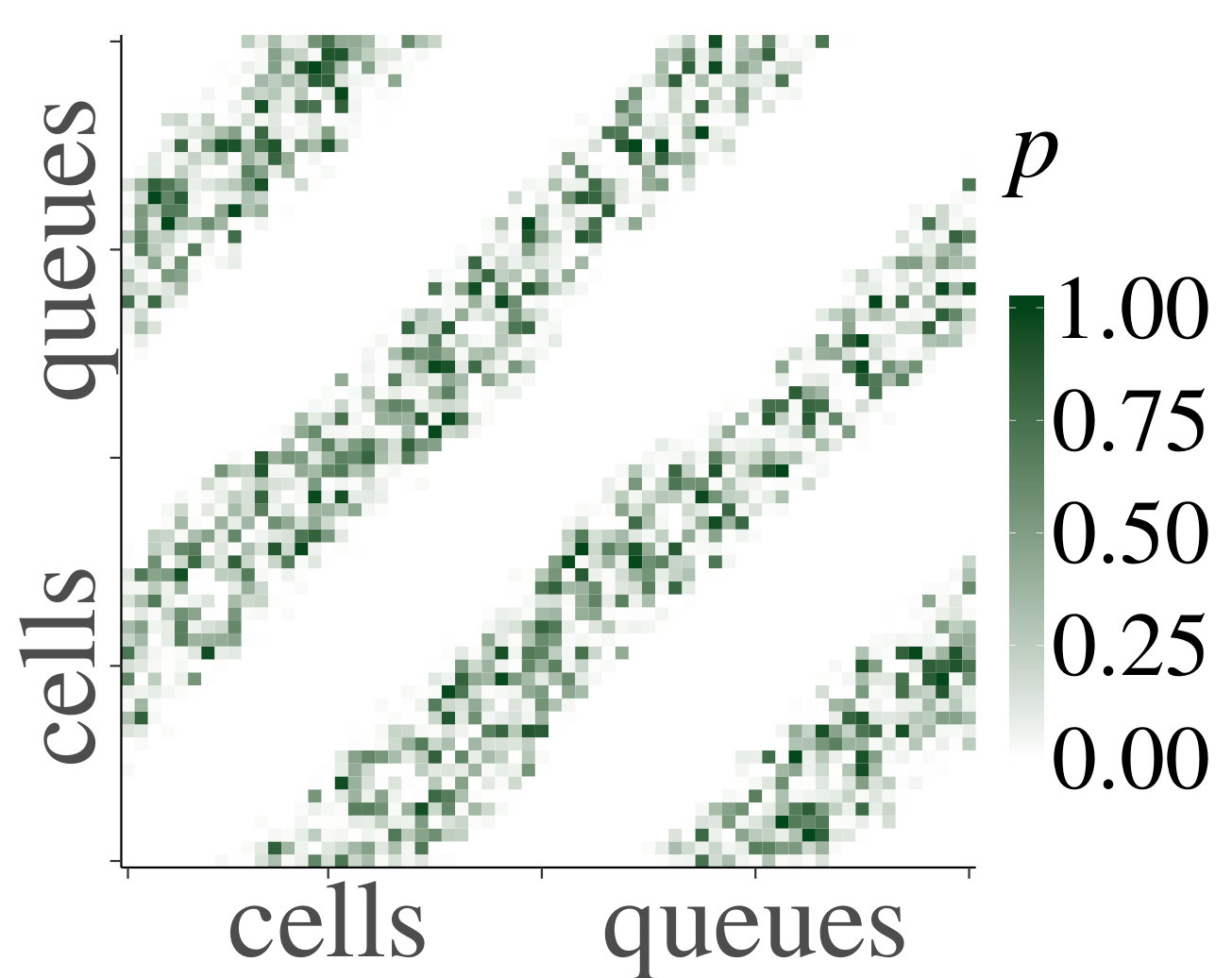 Figure 18
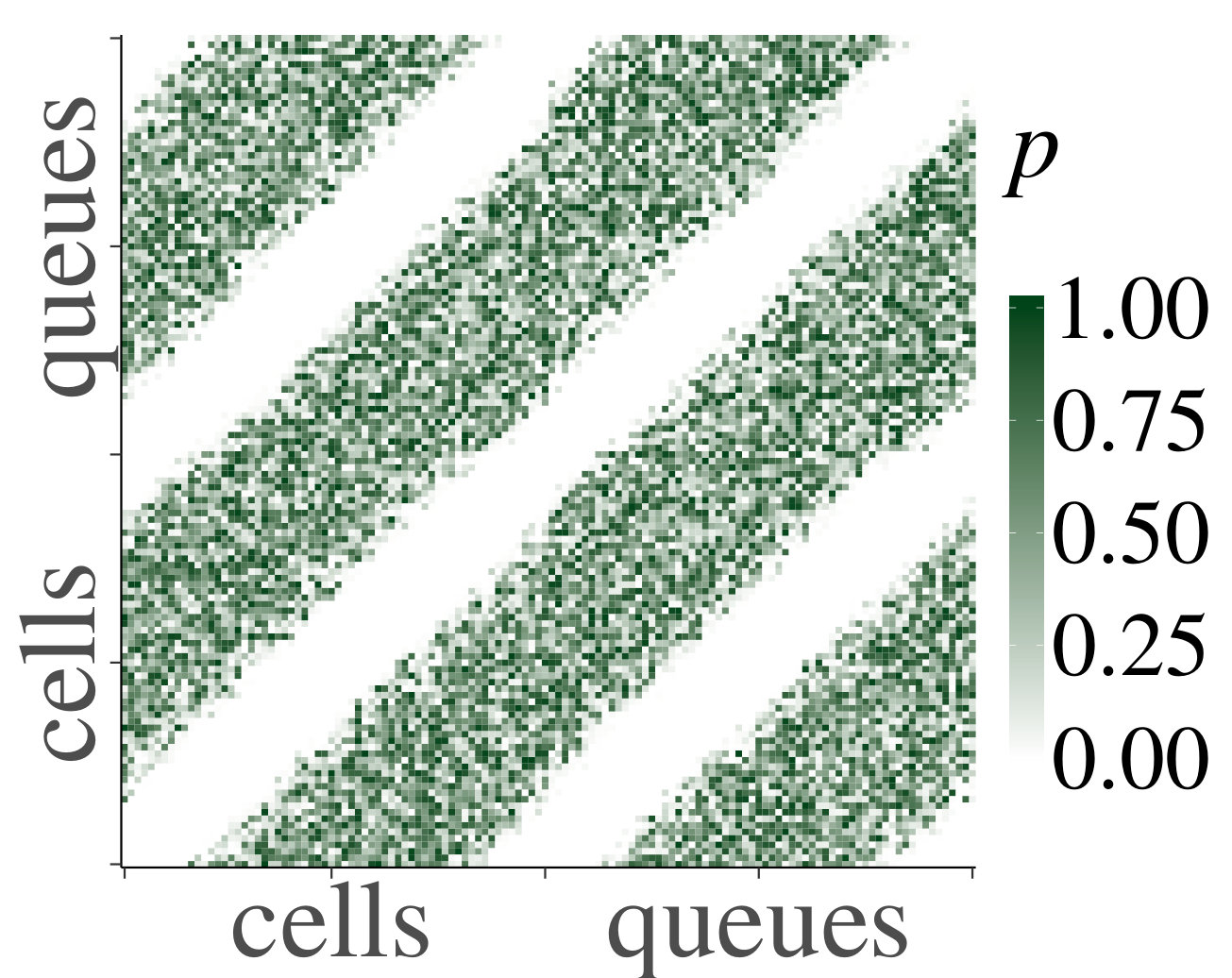 Figure 19
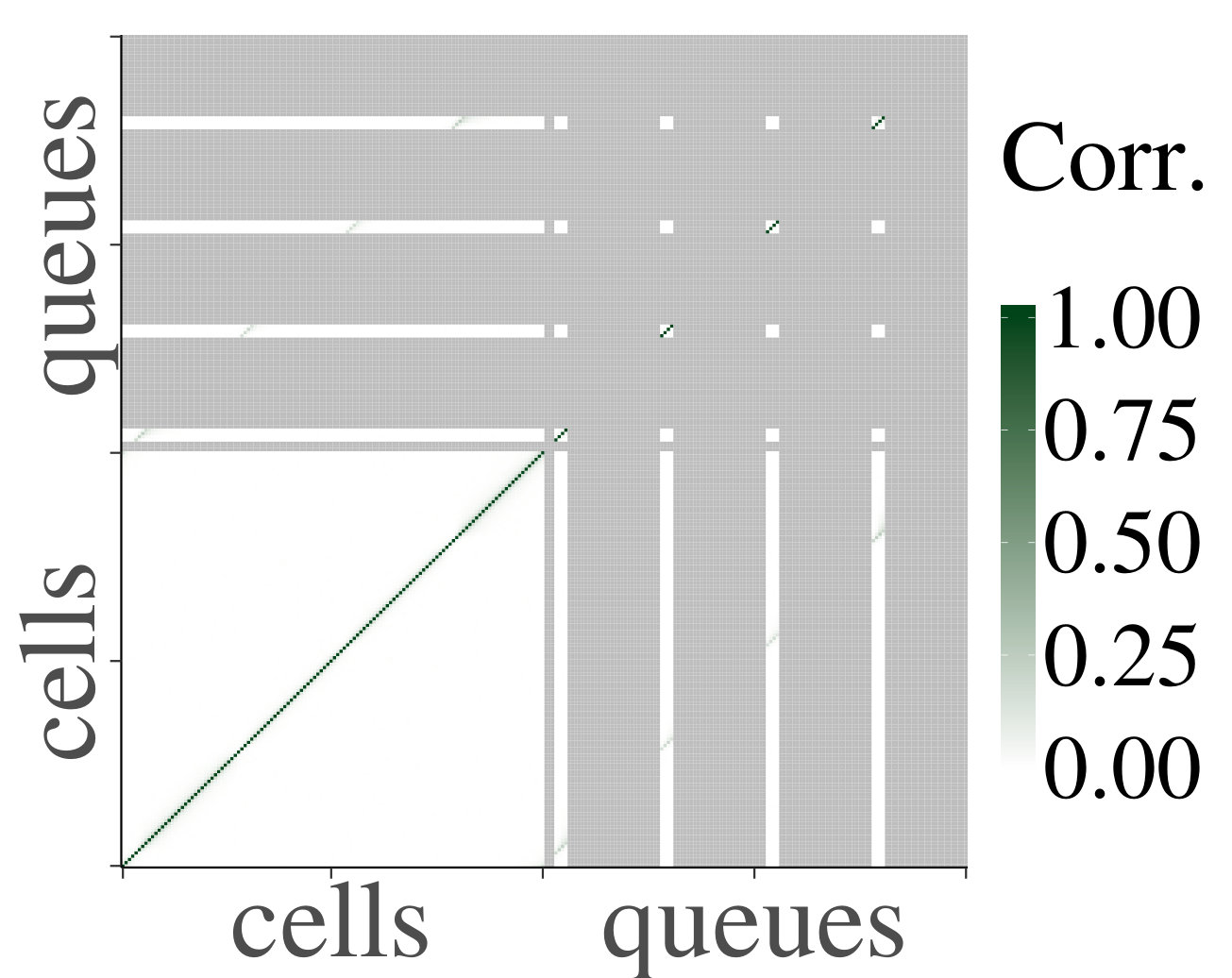 Figure 20
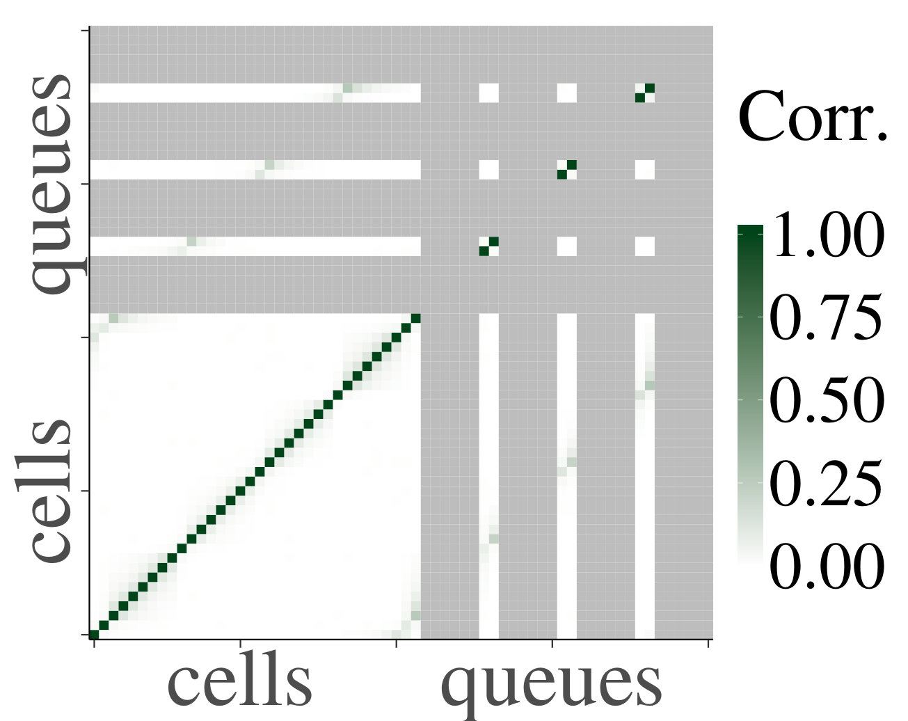 Figure 21
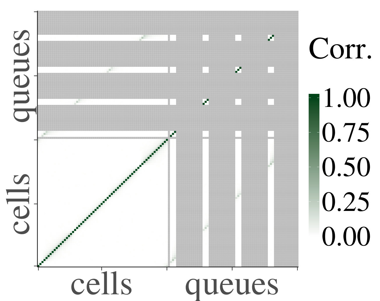 Figure 22
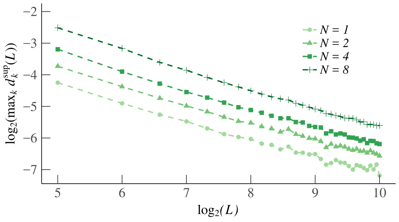 Figure 23
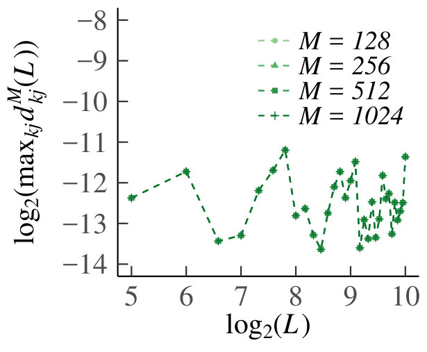 Figure 24
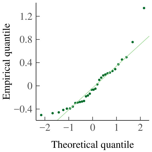 Figure 25
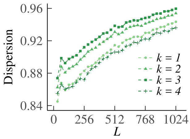 Figure 26
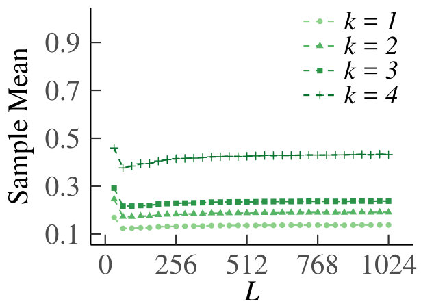 Figure 27
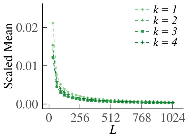 Figure 28
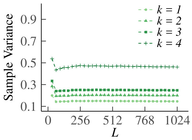 Figure 29
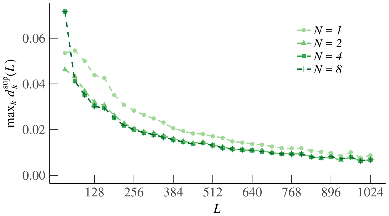 Figure 30
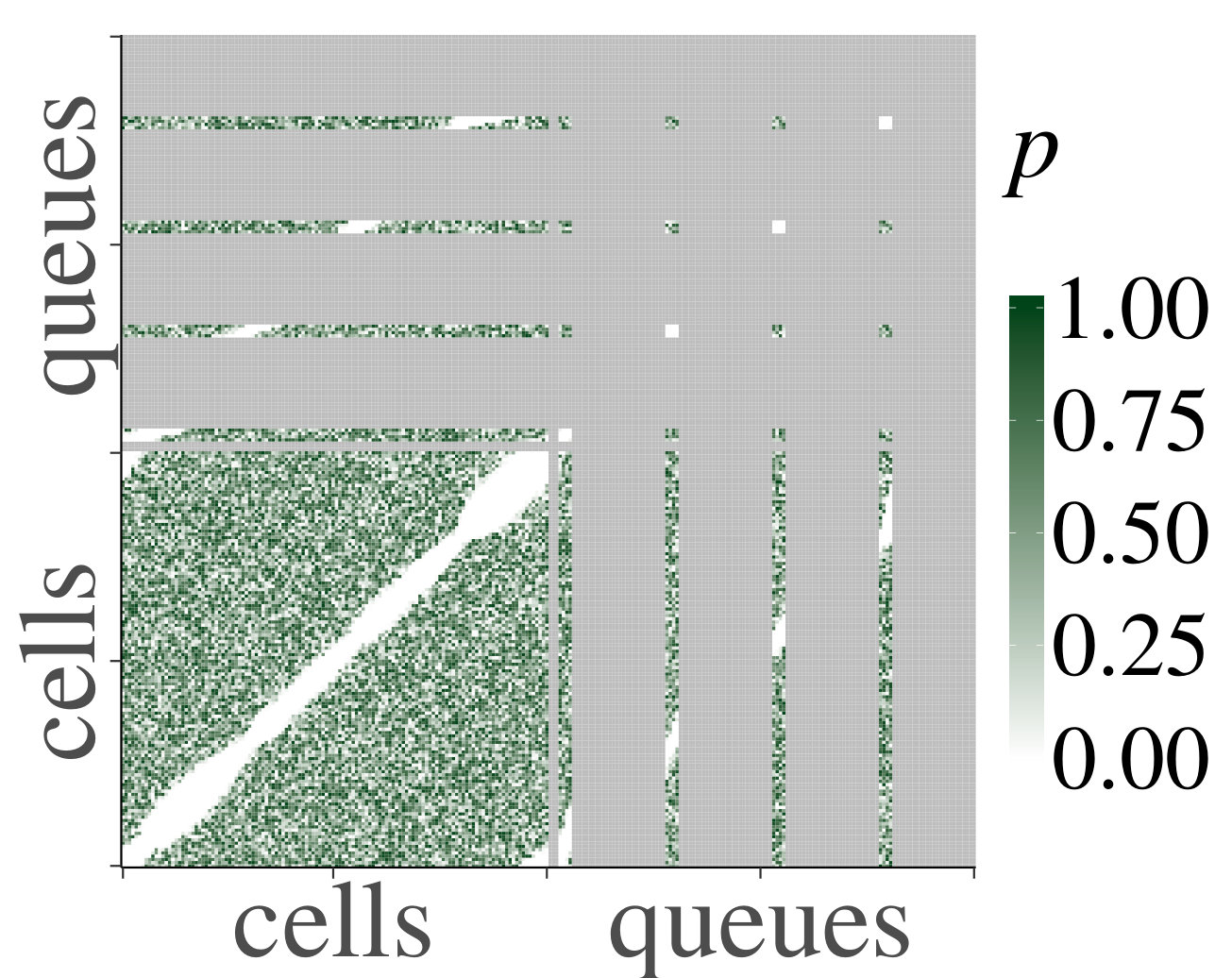 Figure 31
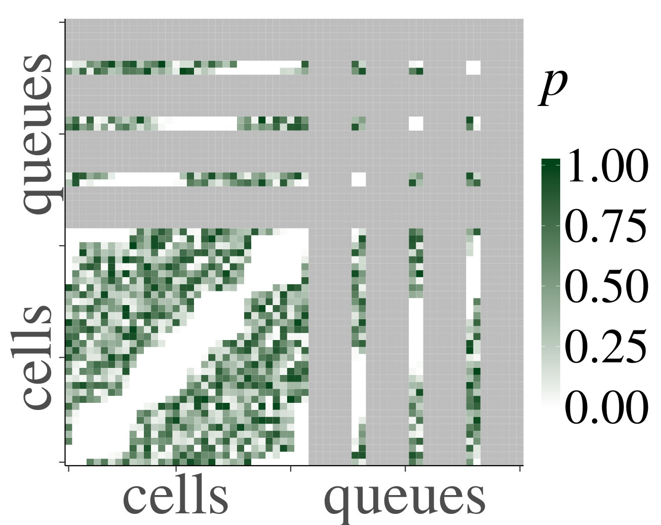 Figure 32
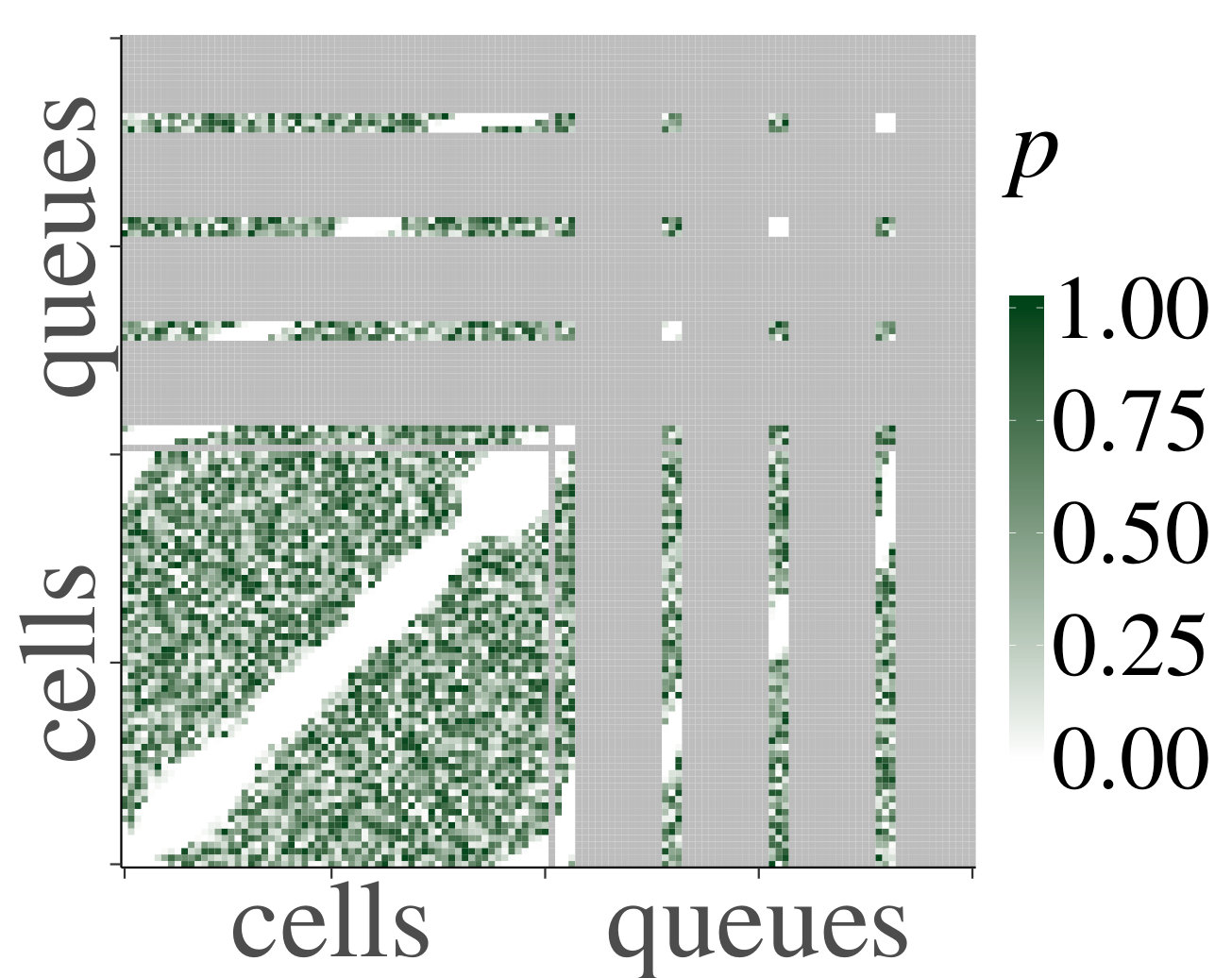 Figure 33
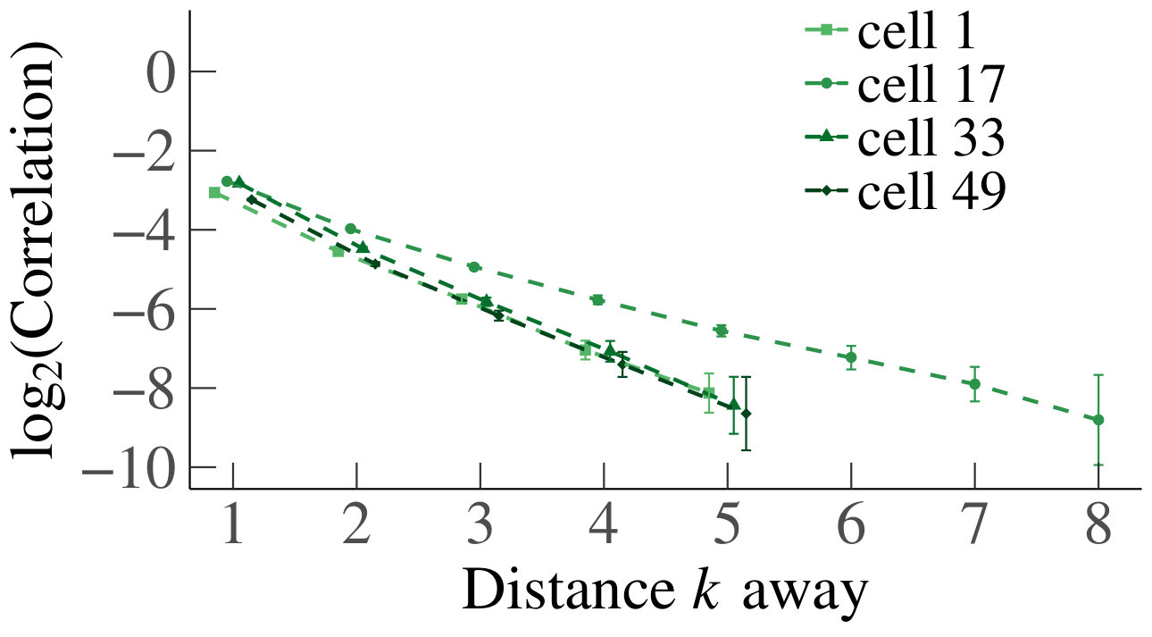 Figure 34
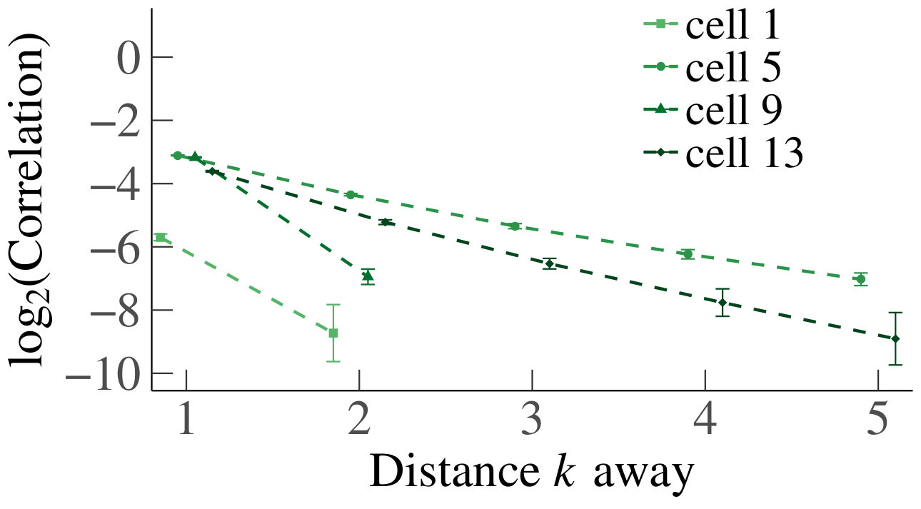 Figure 35
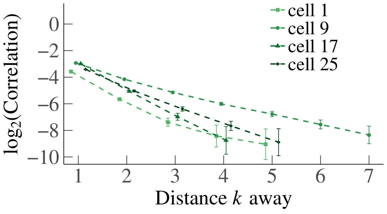 Figure 36
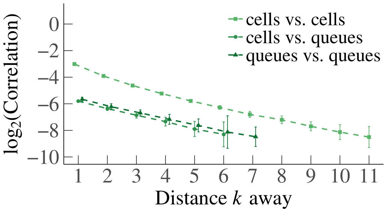 Figure 37
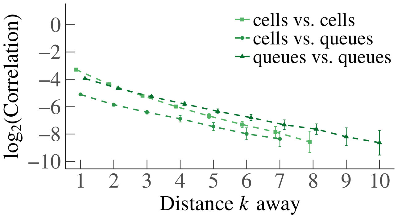 Figure 38
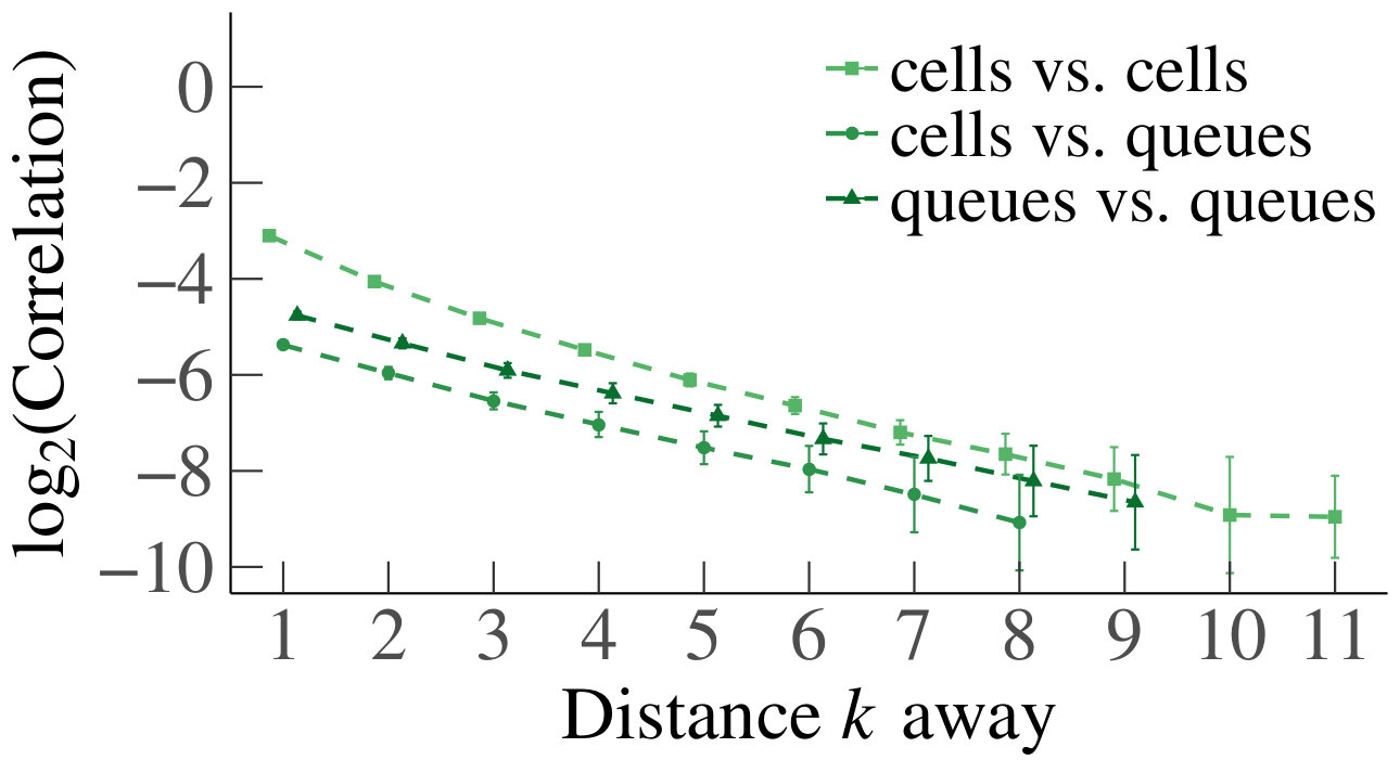 Figure 39
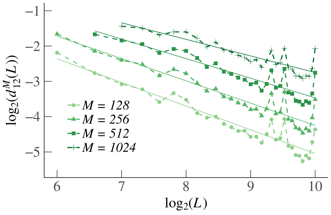 Figure 40
| Rsq | Rsq_adj | intercept | slope | ||||
|---|---|---|---|---|---|---|---|
| 1 | 1 | 0.8134 | 0.8072 | 130.7484 | 1.8457e-12 | 1.0406 | 1.0076 |
| 2 | 1 | 0.7128 | 0.7033 | 74.4703 | 1.2586e-09 | 0.7283 | 1.0261 |
| 2 | 2 | 0.7197 | 0.7104 | 77.0325 | 8.7121e-10 | 0.7331 | 1.0274 |
| 4 | 1 | 0.5816 | 0.5677 | 41.7071 | 3.9042e-07 | 1.4803 | 0.7842 |
| 4 | 2 | 0.5690 | 0.5546 | 39.6035 | 6.1631e-07 | 1.3822 | 0.8033 |
| 4 | 3 | 0.5728 | 0.5586 | 40.2324 | 5.3689e-07 | 1.4932 | 0.7814 |
| 4 | 4 | 0.5797 | 0.5657 | 41.3778 | 4.1895e-07 | 1.4924 | 0.7811 |
| 8 | 1 | 0.5509 | 0.5359 | 36.8022 | 1.1580e-06 | 0.1515 | 0.9281 |
| 8 | 2 | 0.5479 | 0.5328 | 36.3542 | 1.2841e-06 | 0.1686 | 0.9252 |
| 8 | 3 | 0.5435 | 0.5282 | 35.7116 | 1.4914e-06 | 0.1776 | 0.9237 |
| 8 | 4 | 0.5498 | 0.5348 | 36.6344 | 1.2036e-06 | 0.1872 | 0.9214 |
| 8 | 5 | 0.5462 | 0.5311 | 36.1087 | 1.3594e-06 | 0.1447 | 0.9289 |
| 8 | 6 | 0.5428 | 0.5275 | 35.6145 | 1.5257e-06 | 0.1627 | 0.9269 |
| 8 | 7 | 0.5497 | 0.5346 | 36.6159 | 1.2088e-06 | 0.1582 | 0.9277 |
| 8 | 8 | 0.5321 | 0.5165 | 34.1113 | 2.1793e-06 | 0.3014 | 0.8971 |
| Rsq | Rsq_adj | intercept | slope | ||||
|---|---|---|---|---|---|---|---|
| 1 | 1 | 0.7541 | 0.7459 | 92.0002 | 1.1971e-10 | 0.7161 | 1.0702 |
| 2 | 1 | 0.6878 | 0.6773 | 66.0790 | 4.4923e-09 | 0.5324 | 0.9724 |
| 2 | 2 | 0.5639 | 0.5493 | 38.7879 | 7.3848e-07 | 2.0480 | 0.7580 |
| 4 | 1 | 0.7518 | 0.7436 | 90.8835 | 1.3761e-10 | 0.9568 | 0.8230 |
| 4 | 2 | 0.6827 | 0.6721 | 64.5423 | 5.7407e-09 | 0.3722 | 0.8814 |
| 4 | 3 | 0.6955 | 0.6854 | 68.5310 | 3.0624e-09 | 0.3669 | 0.8900 |
| 4 | 4 | 0.7479 | 0.7395 | 88.9982 | 1.7462e-10 | 0.9977 | 0.8228 |
| 8 | 1 | 0.6871 | 0.6767 | 65.8841 | 4.6332e-09 | 1.0612 | 0.6820 |
| 8 | 2 | 0.6306 | 0.6183 | 51.2062 | 5.8243e-08 | 0.8349 | 0.7562 |
| 8 | 3 | 0.4906 | 0.4737 | 28.8981 | 8.0635e-06 | 1.3538 | 0.6137 |
| 8 | 4 | 0.4476 | 0.4292 | 24.3093 | 2.8351e-05 | 1.6853 | 0.5714 |
| 8 | 5 | 0.4880 | 0.4709 | 28.5930 | 8.7378e-06 | 1.5911 | 0.5810 |
| 8 | 6 | 0.4839 | 0.4667 | 28.1235 | 9.8957e-06 | 1.4242 | 0.6184 |
| 8 | 7 | 0.6181 | 0.6053 | 48.5450 | 9.6884e-08 | 0.7438 | 0.7548 |
| 8 | 8 | 0.6540 | 0.6425 | 56.7122 | 2.1412e-08 | 0.6693 | 0.7848 |
Peer Reviews
No public reviews on file for this paper yet. If you reviewed it on a platform where reviews are public (OpenReview, ICLR, NeurIPS, ICML), you can paste yours below so the community can read it here.
Videos
No videos yet. Explain this paper in a talk, walkthrough, or lecture? Add one.
\newaliascnt
claimdummy \aliascntresettheclaim
\newaliascntpropositiontheorem \aliascntresettheproposition
\newaliascntremarktheorem \aliascntresettheremark
A roundabout model with on-ramp queues: exact results and scaling
approximations
P.J. Storm, S. Bhulai, W. Kager
Vrije Universiteit, Amsterdam
M. Mandjes
University of Amsterdam
Abstract
This paper introduces a general model of a single-lane roundabout, represented as a circular lattice that consists of cells, with Markovian traffic dynamics. Vehicles enter the roundabout via on-ramp queues that have stochastic arrival processes, remain on the roundabout a random number of cells, and depart via off-ramps. Importantly, the model does not oversimplify the dynamics of traffic on roundabouts, while various performance-related quantities (such as delay and queue length) allow an analytical characterization. In particular, we present an explicit expression for the marginal stationary distribution of each cell on the lattice. Moreover, we derive results that give insight on the dependencies between parts of the roundabout, and on the queue distribution. Finally, we find scaling limits that allow, for every partition of the roundabout in segments, to approximate 1) the joint distribution of the occupation of these segments by a multivariate Gaussian distribution; and 2) the joint distribution of their total queue lengths by a collection of independent Poisson random variables. To verify the scaling limit statements, we develop a novel way to empirically assess convergence in distribution of random variables.
pacs:
I Introduction
Over the past decades, a broad class of models has been proposed to better understand and control traffic streams in road traffic networks. This has led to mathematical models that help shed light on the properties of the underlying traffic dynamics. In particular, these models allow for studying the influence of the model’s parameters, which in turn allows for developing effective design and control rules. For reviews on traffic flow theory, see, e.g., Maerivoet and De Moor (2008); van Wageningen-Kessels et al. (2015), and for cellular automata models used in this area, see Maerivoet and De Moor (2005). In the literature on traffic flows, most mathematical analyses are done for road segments and several forms of intersection traffic control, i.e., signalized intersections and unsignalized intersections with or without priorities.
Roundabouts are a type of intersection that is notoriously hard to analyze mathematically. Fouladvand et al. Fouladvand et al. (2004) studies the delay experienced by traffic on roundabouts in relation to their geometry by simulating a stochastic cellular automata model. Wang and Ruskin Wang and Ruskin (2002), Wang and Liu Wang and Liu (2005), and Belz et al. Belz et al. (2016) study the capacity of cellular automata roundabout models incorporating the traffic behavior of individual cars in a more sophisticated manner. In these models, the analysis focuses on the relationship between the circulating flow, and the capacity of an entry road at the roundabout. The conclusions are primarily based on simulation results, and hence do not provide explicit insight into, e.g., the way the system parameters affect the capacity or delay.
In addition, there are a number of analytical papers studying the relationship between circulating flow and capacity at an entry road. For example, Flannery et al. Flannery et al. (2000, 2005) have obtained an analytical approximation of this relationship based on earlier work for unsignalized intersections by Tanner Tanner (1962) and Heidemann and Wegmann Heidemann and Wegmann (1997). For these results, vehicles are assumed to be separated by i.i.d. distributed gaps, so that on-ramps can be modeled as queues. However, this approach studies queues in isolation, and ignores the interaction of on-ramps being connected to a circular ring. Finally, in a recent paper, Foulaadvand et al. Foulaadvand and Maass (2016) derive exact stationary densities for the occupation of a roundabout, with traffic motion modeled by the totally asymmetric exclusion process, but, importantly, without queueing at the entry roads.
Summarizing, many studies are based on simulation models or regression analyses (HCM2010, 2010, Ch. 21), thus not providing direct insight into the impact of the model parameters. On the other hand, analytical studies tend to study parts of the roundabout in isolation, ignoring characteristic geometric properties of roundabouts. The primary contribution of this paper is a single-lane roundabout model that (1) is still analytically tractable, and (2) still contains the detailed geometric properties of the underlying system. More specifically, we set up a model in which we succeed to derive (a) an exact marginal stationary distribution for the occupation of the roundabout; (b) results on the dependencies between parts of the roundabout, and on the queue distribution; (c) scaling limits for the occupation of the roundabout and the states of the queues. Our results lead to a better understanding of traffic dynamics on roundabouts, and, in particular, of the effects of model parameters on performance. As a consequence, our findings have evident application potential when setting up procedures for design and control. A second main contribution relates to the verification of properties (b) and (c) above, for which we rely on simulation: we develop a novel procedure to statistically assess convergence in distribution.
The outline of the paper is as follows. In Section II, we introduce the model. In Section III, we identify the exact marginal stationary distribution for the occupation of the roundabout, and discuss why it is difficult to derive further analytic results. Our methods, which are used in later sections, are explained in Section IV. Section V contains results on intrinsic model properties, whereas in Sections VI and VII we study scaling results.
II Model Description
The model we consider is a road traffic model for a roundabout with (on-ramp) queues at the points of entrance onto the roundabout. The exit point of a car from the roundabout is random and depends on its point of entry. The roundabout is modeled as a stretch of road consisting of cells numbered , which we assume to be arranged in a circle, so that cell 1 is adjacent to cell . Making use of this circularity, we will also use the index to refer to cell , for , to simplify notation. Each cell can contain at most one car, and to keep track of the cars on the roundabout, we attach the state space to each cell: state [math] indicates that a cell is vacant, and a state indicates that the cell is occupied by a car that entered the roundabout at cell . For ease of reference, we will also say that a cell is occupied by a car of type if the state of the cell is .
The main characteristics of the evolution of our stochastic system are the following. To model how cars get onto the roundabout, we assume that there is an on-ramp queue in front of each cell . At every time step, a new car arrives at the queue of cell with probability . From this queue, in every time step, a single car can move onto the roundabout, but only when cell is empty. If cell is occupied by a car of type at a specific moment in time, then with probability the car will leave the roundabout in the next time step (and otherwise it moves to the next cell). The fact that the probability depends on reflects that, in general, the position where a car leaves the roundabout can depend on where it entered. Note that by setting or we can remove on-ramps and off-ramps from the system, and thus flexibly model their position.
Now that we have sketched the main principles behind our model, we proceed by providing a more precise account of the dynamics. A key feature of the model is that the update rules (given in detail below) are local, meaning that at each time step, we can consider what happens at each of the cells of the model independently, and then update all the local states in parallel (in accordance with the cellular automata paradigm). Thus it suffices to describe what happens at a single cell and the corresponding queue. We distinguish between the following cases:
Case 1:
cell and queue are both empty. In this case, if no new car arrives at cell (which happens with probability ), then cell and queue will both be empty at the next time step. Otherwise, the newly arrived car immediately enters the roundabout and moves on to cell , meaning that cell will be in state at the next time step, and queue will still be empty.
Case 2:
cell is empty and queue is not empty. In this case, the first car waiting in queue enters the roundabout and moves on to cell . Thus, cell will be in state at the next time step, and the length of queue will either decrease by one (if no new car arrives at cell ), or otherwise stay the same.
Case 3:
cell is occupied by a car of type . In this case, queue is blocked, and hence its length will stay the same if no new car arrives at cell , or otherwise grow by one. Meanwhile, the car of type can decide to leave the roundabout (which it does with probability ), in which case cell will be empty at the next time step, or the car decides to drive on, in which case cell will be in state at the next time step.
III Preliminaries
The model under consideration is a discrete-time Markov chain, the state of which is a vector describing the state of each cell and the length of each queue. We will denote the Markov chain by . It is not difficult to see that is irreducible and aperiodic, since with positive probability, by choosing the right events, we can empty the system in a finite number of steps, keep it in the empty state for an arbitrary number of steps, and then send it to any state we like in a finite number of steps.
We say that the model is stable if the Markov chain is positive recurrent, and hence has a unique stationary distribution. As our first result, we will now show that, under the assumption of stability, the marginal stationary probability that a given cell is in state is given by
[TABLE]
where , and
[TABLE]
Proposition \theproposition (Marginal stationary distribution).
If the model is stable, then the marginal stationary probability that cell is in state is given by (1)–(2).
Proof.
Assume that the model is stable, and first consider the case that and satisfy . Then the probability that a car that enters the roundabout at cell will leave at cell (potentially after first completing full circles on the roundabout) is given by
[TABLE]
We conclude that this expression multiplied by is the rate at which cars arrive that are of type , and that intend to leave the roundabout at cell . But if the model is stable, then the rate at which such cars leave the system must be equal to , where denotes the marginal stationary probability that cell contains a car of type . This proves (1) when . The proof in the case is similar. ∎
Even though we now have an exact expression for the marginal stationary distribution of the cells, the full joint stationary distribution of the Markov chain cannot be found. In particular, the stationary distribution will not be the product distribution of the marginals of the cells and queues. Indeed, consider the event that queue and cell are both empty for some . Then, one time unit earlier queue must have been empty, because otherwise, either queue would now still be non-empty, or a car from queue would now be in cell . This shows that there is a dependency in the model between adjacent cells and queues, ruling out a product-form stationary distribution.
To conclude this section, we discuss the model’s stability condition. We have shown above that when the model is stable, is the stationary probability at which cell is empty. Since cars arrive at cell with probability , and can only enter the roundabout when the cell is empty, it is conceivable that the model cannot be stable if for some cell . Conversely, one suspects that if for all cells , then the cells will be vacant often enough to prevent the queue lengths from growing arbitrary large, and hence the model will be stable. We have tested this conjecture using extensive simulation experiments in which we replace by and increase (starting from ). The experiments confirm that a system becomes unstable when exceeds the smallest value for which for some . Throughout Sections IV–VII, we therefore restrict ourselves to cases where for all .
IV Methods
Since we do not have a closed-form expression for the joint stationary distribution, we resort to finding approximations for the stationary distributions of cells and queues. More specifically, in Section II we introduced the and , which can be seen as discrete profiles of arrival and departure probabilities (as a function of the position between and ). In Section IV.1, we introduce their continuous counterparts, so that for finite , the and are obtained as discretizations of these continuum profiles. The continuous setting allows explicit analysis, with which we can approximate our discrete model.
Later in the paper (in Sections VI and VII) we state claims on, respectively, the number of empty cells and total queue length for each section of the roundabout in the regime . To verify these claims from simulation experiments, we develop a novel methodology, which is described in Section IV.2.
IV.1 Continuum Profiles and Parameters
We proceed by introducing the continuum profiles of arrivals and departures. We start with the arrivals. Let be an integrable function that satisfies . For given , , and , we set
[TABLE]
This construction can be interpreted as follows. When taking the limit , the circular stretch of road is mapped onto the unit interval . The parameter represents the total rate at which cars arrive at the roundabout, and for a given interval , represents the rate at which cars arrive in that interval. Informally, for large, is roughly proportional to . Note that in this setup, the arrival rate over every segment of the roundabout is invariant in .
To describe the continuum profile for the departures, we introduce a family of cumulative distribution functions on (which are non-decreasing with ), and denote by their complementary distribution functions. The idea is that in the limit , represents the probability that a car that enters the roundabout at point , travels at least a distance along the roundabout before leaving. For each finite and , we now set
[TABLE]
Since we interpret as the distribution function of the driving distance for cars arriving at , for can be seen as the conditional probability that such a car drives at least distance on the roundabout, given that the car has driven distance , and similarly for . Hence the above definition of the guarantees that the distribution of driving distance of cars remains invariant in . We further assume that is piecewise continuous as a function of , meaning that cars that arrive at roughly the same place on the roundabout, also have roughly the same distribution of driving distance. This condition is natural, and guarantees the existence of .
To summarize: for given and a family of , we obtain a sequence of models in , which can be viewed as discrete representations of the same roundabout. In the remainder of the paper, we consider two specific cases of continuum profiles and the discrete models they produce for different values of , in order to support the claims we make in Sections V, VI, and VII.
Most of the arguments by which we arrive at our claims are based on the symmetric case where and for each . We therefore choose a parameter setting in this symmetric case such that . More specifically, we choose with , and for each , so that for finite we have and . We refer to this choice as the homogeneous setting or homogeneous case.
To illustrate that our claims are also supported in a realistic non-homogeneous case, we use an example from (HCM2010, 2010, Ch. 21), namely Example Problem 1. This example describes a roundabout with four on/off-ramps, and gives for each on-ramp (1) the number of arrivals per hour, and (2) the fraction of arriving cars that depart via each of the four off-ramps. To choose a and family of that correspond to this example, we start by calibrating a finite model that has a realistic size. Using the calibration in (Belz et al., 2016, Section 3.1), we take the length of each cell to be about 7 meters and our time steps to be 1 second, and find that is a suitable choice. The resulting model has geometric features and car velocities that match the realistic ones described in HCM2010 (2010) and Akçelik (2011). We let the on/off-ramps be located at cells , meaning that only these cells will have non-zero arrival and departure probabilities, while we set the remaining and to zero. We calculate the arrival probabilities at the four on-ramps from the given number of arrivals per hour in the example problem. The departure probabilities are analogously obtained from the given fractions of arriving cars that depart via the off-ramps. The latter requires that we first fix the probability that a car completes a full circle on the roundabout; we set this probability equal to for every type of car, and then determine the to reproduce the departure behavior of the example.
Now that we have the and for , we can choose our continuum profiles and accordingly. Recall that we map the full roundabout to the interval , so that for , each cell corresponds to an interval of length . We further split each of the four cells into two halves, where the half that is adjacent to the previous cell corresponds to the off-ramp of the cell, and the other half to the on-ramp. We now choose proportional to at the on-ramps and zero elsewhere, and we choose , so that for , integration of gives us the correct . As for the departure profiles, we choose the to be exponentially decreasing at the off-ramps in analogy with the homogeneous case, and constant in between. Here, the rate of the exponential decrease is chosen such that we obtain the correct for . In Fig. 1 we have plotted the resulting profiles and a representative from the family for illustration. We refer to the profiles and thus obtained as the heterogeneous setting or heterogeneous case. We stress that, although these profiles were calibrated for , we use the same and in our simulations of the heterogeneous case for other values of .
In the remainder of the paper, we present various claims about the model. We cannot prove these claims, as we lack an analytic expression for the joint stationary distribution. Instead, we will support our claims using simulation in combination with statistical evidence. We throughout use the following structure: first we state the claim and give intuition behind it based on properties of the model, then we describe an experiment by which we aim to support the claim, provide our support, and finally, we draw our conclusions. In each simulation experiment, we initialize (1) the cells according to the marginal stationary probabilities , and (2) the queues empty. We then let the system run for units of time, as we have observed that this is a sufficiently long time interval to safely assume the system has entered the stationary regime.
IV.2 Supporting Convergence in Distribution Statistically
In Section VI, we consider the number of empty cells on a segment, for a sequence of models in that we obtain from the continuous arrival and departure profiles, as explained in the previous section. Among other things, we claim that this quantity converges in distribution to a normal random variable as . To empirically verify this claim, we use two methods. The first, which is classical, is to show that the (empirical) distribution functions converge pointwise. The second uses statistical tests and is, to the best knowledge of the authors, a novel method to numerically support convergence in distribution. We explain the second method in this section.
For our explanation, we consider the situation where is a sequence of random variables that converge in distribution to a random variable. In our method, we use the chi-squared goodness-of-fit test with a confidence level equal to . We take 10 bins, the boundaries of which are chosen such that every bin contains of the probability mass of the distribution.
The naive idea for testing convergence to a normal distribution would be to take large, and apply the -test with the (-dependent) hypotheses
[TABLE]
However, a -test with these hypotheses does not give useful information on convergence because, in practice, one expects that does not have a distribution for finite , and therefore, one will always reject if the sample size is large enough. The underlying issue is of course that to support convergence in distribution, it is not sufficient to consider a single , but one has to consider the full sequence. Our method exploits the fact that we can always reject by increasing the sample size. The basic idea is that we compare the sample sizes for which we first reject . If converges in distribution, should diverge to with .
To put this idea into practice, we start our procedure by drawing a sample of independent copies of . We perform the chi-squared test for goodness-of-fit, with the hypotheses as in (3), which is significant for samples (taking into account the expected counts in each bin). If we reject , we set ; otherwise, we add another independent copy of to our sample, and perform the chi-squared test again. We keep adding independent copies of until we reject , at which point we record the size of our sample . Note that is itself a random variable, so we run this procedure multiple times to estimate the mean . Finally, we use linear regression to test whether increases like a power law with , which implies that as , a diverging number of samples is required to reject , thus supporting convergence in distribution.
Our method can, in theory, be applied to every limiting distribution with a set of hypotheses as in (3), using any goodness-of-fit test. For practical applications, however, one has to be able to compute an estimate of . For instance, in Section VII, we claim convergence in distribution of the total queue length on a segment to a Poisson random variable. There is, however, no statistical test that is powerful enough to distinguish the specific alternative distribution that we are considering. Therefore, one has to use a huge sample size to reject , even for small , which makes estimating the computationally infeasible in this particular case.
V Model Properties
In this section, we study the spatial correlations and marginal queue distributions of our model in the finite regime in equilibrium. Our results also provide information about the behavior in the regime , which we study in more detail in Sections VI and VII.
V.1 Spatial Correlations
Our roundabout model can be seen as a system of particles moving over a one-dimensional circular lattice. Moreover, the update rules are local, so that correlations in the model arise via nearest-neighbor interactions. It is, therefore, conceivable that the correlations decay geometrically in the distance between cells. To investigate this idea, denote by the state of cell and by the state of queue in equilibrium. In order for states of the cells to contribute symmetrically to the correlations, we let
[TABLE]
when , and if . Thus, measures the forward distance to the cell where the car that occupies cell entered the roundabout. Now, our claim is as follows:
Claim 1**.**
The correlation between the random variables and decreases in for each , and is bounded above, uniformly in both and , by a function that decreases geometrically with . The same statement is true for the correlations between and , and for the correlations between and .
To support Claim 1 it is sufficient for the sample correlation to be geometrically decreasing, starting from some distance . To verify this, we estimate the mean sample correlation coefficient between pairs of cells and/or queues, from a sample of 100 correlation coefficients, each estimated from a simulated data set of size . To analyze the decay of the, potentially negative, mean sample correlation coefficient on a log scale, we take the absolute value of the 100 samples and consider their mean. We then verify that on a log scale, these mean absolute sample correlations are bounded by a decreasing linear function. However, from known results on the asymptotic distribution of the sample correlation (Kendall and Stuart, 1961, Example 10.6), we expect that the variance becomes constant as the correlation tends to zero. As a consequence, in our experiment, the mean absolute sample correlation will not be a good estimator of the absolute correlation when the correlation is small. To ensure that our estimates are accurate, we therefore only consider points for which the mean sample correlation is at least two standard errors (as determined from the 100 samples) away from zero.
If the correlations do decay geometrically, cells and/or queues that are ‘sufficiently far apart’ are approximately independent. To verify this, we also perform a statistical test of independence. We use the statistic , where is the correlation coefficient, and is the sample size. For generally distributed independent random variables and large , the statistic can be shown to have a Student’s distribution with degrees of freedom (Kendall and Stuart, 1961, Section 26.20). In our experiment, we take and use to test whether the sample correlations are significant. We aim to show that the correlations are significant over a constant distance independent of , thus further supporting the claim of geometric decay, uniformly in .
Support** (of Claim 1).**
We consider the homogeneous case first. In Fig. 2 we show heatmaps of the correlations and their corresponding p-values between cells and queues for . Both axes represent a vector containing first the cells, indexed from 1 through , and then the queues, indexed from 1 through . First of all, notice that non-trivial correlations do exist, and that for each they are significant for certain pairs of cells and queues. This confirms that a product-form stationary distribution does not apply, as pointed out earlier. However, we also see that the dependence is not very strong, since (although they are significant according to the p-values) the correlations between neighboring cells and/or queues are small. Furthermore, we observe that p-values are only significant for correlations between cells and queues that are at most (about) distance 10 away from each other. This distance is more or less constant in , which supports our claim that the rate of the decay is uniform in .
In Fig. 3 we have plotted the mean absolute value of the sample correlations between a cell/queue and neighboring downstream cells and/or queues, for starting from distance , with the corresponding standard error represented by error bars. We have tested for a linear relationship, by applying linear regression, yielding for every line. We therefore deduce that the decrease is linear, and we can conclude that the mean absolute correlations decay geometrically. Furthermore, we see that the behavior is homogeneous in . Based on the above, we conclude that our experiments support Claim 1 numerically in the homogeneous case.
For the heterogeneous case, we likewise present a set of heatmaps of the correlations and their corresponding p-values in Fig. 4. As some queues are by construction empty in the heterogeneous case, their correlations are depicted in gray in the heatmaps. As in the homogeneous case, the results of our simulations numerically support Claim 1. To analyze the decay of the correlations, we have also plotted on a log scale, for the first four cells that are a distance apart from each other, their mean absolute correlations with neighboring upstream cells, and their standard errors, as a function of the distance; see Fig. 5. We have applied linear regression, which gave for every graph, except for the graph of cell 1 for , which has . The results confirm a linear decay on a log scale. Therefore, as in the homogeneous case, we find numerical support for Claim 1.
V.2 Queue distribution
A natural quantity to study is the (marginal) queue length distribution of the system. Because of the dependencies in the system, one cannot derive the marginal queue length distribution analytically; likewise, no mean-value analysis is possible to capture the mean queue length. However, because of the weak dependence, one would expect the queue distribution to approximately have a geometric tail. We, therefore, claim the following:
Claim 2**.**
All queues have marginal stationary distributions with a tail that is close to geometric.
To verify Claim 2, we have simulated the roundabout for . To estimate the tail of the queue distributions in a sample of size sufficiently accurately, we have to scale the by a factor , in both the homogeneous and the heterogeneous case. We choose such that for each . From our data, we estimate the marginal distributions of a set of queues with equal distance between them, and analyze the tail.
Support** (of Claim 2).**
The results in the homogeneous case are shown in Fig. 6 (left), where on the vertical axis denotes the stationary probability of the event that queue has length . The figure shows the distribution on a log scale along with its regression line. The slight deviation from the linear relation for small shows that the distribution is not exactly geometric. However, we observe that the tail is indeed geometric, as the plot is very close to the regression line and linear in the tail, until the estimation errors kick in, thus confirming Claim 2.
For the heterogeneous case, Fig. 6 (right) shows the results on a log scale. That is, we have plotted the distribution of one queue in each of the four arrival zones (i.e., the four on-ramps on the roundabout) for . The legend indicates which queues are considered. We see that each distribution is close to a linear decay on a log scale for above, say, 4. For , there seems to be a small deviation from a linear line in the tail of the distribution, though performing linear regression yields an equal to . Thus the analysis indicates that, in practice, the distribution can be considered as having geometrically vanishing tails, supporting Claim 2.
VI Scaling Limit for Cells
In this section, we formulate claims about the stationary state of the cells in the regime . More specifically, we claim that for each division of the roundabout into segments, the occupation of these segments follows a joint Gaussian distribution in the limit. This Gaussian limit provides an approximation to the stationary distribution of the number of occupied cells, on every segment of the roundabout. This knowledge is particularly useful when designing the roundabout; for instance, a performance target could concern the maximum utilization of the roundabout.
We first introduce some notation. Let be the random variable that counts the number of vacant cells up to cell : with the state of cell , and the Kronecker delta (i.e., if , and if ),
[TABLE]
Observe that this is a sum of 0-1 random variables with expectations . For , write and . Put
[TABLE]
and
[TABLE]
Now let be the random continuous function that is linear on each interval , , and has values
[TABLE]
at the points of division. Then our claim is as follows:
Claim 3**.**
As , converges in distribution to a time-inhomogeneous Brownian motion on with the representation
[TABLE]
interpreted as an Itô integral with respect to a standard Brownian motion , where is a deterministic continuous function on .
We write ‘time-inhomogeneous’, where obviously in this context ‘time’ refers to the position on the roundabout.
Remark \theremark.
Instead of counting vacant cells, one could also count cells containing a car of a type between and , for fixed and satisfying . The corresponding random continuous function again converges to a time-inhomogeneous Brownian motion.
The intuition behind the claim is as follows. If the 0-1 variables in the definition of were independent, would converge to standard Brownian motion by an extension of Donsker’s theorem (Billingsley, 2013, Exercise 8.4). Unfortunately, as stressed before, the cells are not independent. However, we have seen in Section V that the correlations between cells are geometrically decaying in the distance between them, and that cells that are ‘sufficiently far apart’ are nearly independent. Hence, one still expects convergence to a (time-inhomogeneous) Brownian motion.
In particular, we expect that non-overlapping increments of the random function become asymptotically independent (as grows). Moreover, since the central limit theorem still holds for sequences of random variables that are nearly independent when they are far away from another (e.g., see (Billingsley, 2008, Thm. 27.4) for the stationary case), we expect that the increments converge in distribution to zero-mean normal random variables.
As for the covariance matrix between increments, we expect first of all that
[TABLE]
where is a constant representing the row average of all correlations in the upper triangular part of the correlation matrix. This sum should be finite because of the geometric decay of correlations. Finally, we expect that the covariances between increments converge to zero, since
[TABLE]
Here, means that both sides have the same limit as , denotes the correlation coefficient, and the limit is zero since the double sum in the third line is of constant order in by the geometric decay of correlations.
In view of the above, to support Claim 3, we aim to test (1) that increments of become asymptotically independent as , and (2) that they converge in distribution to zero-mean normal random variables.
VI.1 Independence of Increments
To verify that the increments of become independent as , we compare the joint distribution of two increments to the product distribution of the marginals. We divide the roundabout of size into four segments of equal length, and denote the four increments of on these segments by , where and the superscript indicates the dependence on .
As a measure of the distance between the joint distribution of increments and and the distribution one would have if these increments were independent, we define
[TABLE]
Here, the supremum is taken over sets consisting of distinct outcomes of the random vector , is the joint density of and , and and are the respective marginal densities. We note that for , we interpret as and as . To ensure that the product sample space of and has at least elements, must be large enough (to be precise, ). To support Claim 3, we wish to empirically show that for as .
Note that if we replace the supremum in (4) by a supremum over sets of arbitrary size, then (4) becomes the total variation distance. That distance is not suited for our purposes, because we have to estimate the densities in (4), and the total estimation error grows faster than the total variation distance decreases. This is why we restrict the sum to the largest contributions in (4).
In our experiment, we take and evaluate by estimating the densities and using a simulated sample of size .
Support** (of Claim 3).**
We first consider the homogeneous case. Since neighboring increments have a stronger dependence, as shown above, and because of symmetry, the results of are representative for all . Fig. 7 shows the estimated as a function of on a log-log scale, together with the best-fit line. For every , we obtain an between and , and a negative slope. Thus we conclude that for each , the estimated decreases in according to a power law. This is sufficient to also conclude that as , which supports our claim that the increments of become independent as becomes large.
For the heterogeneous case, we have plotted the distance (for different ) in Fig. 8. Our conclusions are the same as in the homogeneous case.
VI.2 Distribution of Increments
We now focus on supporting the part of Claim 3 stating that the increments of converge in distribution to a normal random variable. For this purpose, we divide into intervals of equal length. For fixed , we denote the corresponding increments of by , and their standard deviations by , where . Denote by the cumulative distribution function of a -distribution with degrees of freedom.
We use the two methods described in Section IV.2. However, a complication is that we do not know , and, therefore, do not have a complete description of the limiting distribution. Hence, we slightly modify the two methods by considering the random variables , where is the maximum-likelihood estimator for , estimated from a simulated sample of size . Claim 3 implies that, as , converges in distribution to a random variable that has distribution , and it is this implication that we will support.
With our first experiment, we aim to show that, for every ,
[TABLE]
as , where denotes the supremum norm, and denotes the empirical distribution function of .
In our second experiment, we use the novel method that was explained in Section IV.2. To be precise, we apply the chi-squared goodness-of-fit test, with the hypotheses
[TABLE]
to determine . We estimate by repeating the procedure times, and aim to show that diverges as .
Support** (of Claim 3).**
Consider the first experiment, and the homogeneous case. For , we have plotted in Fig. 9. By symmetry, the results for are similar. As the graphs are all linear in on a log-log scale, the distance decreases in like a power law. This is in turn sufficient to conclude that for each , as , and thus supports Claim 3.
For the heterogeneous case, Fig. 10 depicts the distance as a function of . The results are in line with those of the homogeneous case. Hence, the experiment supports convergence in distribution of the increments of .
Support** (of Claim 3).**
Now consider the second experiment. For and we have estimated the for . Then, we applied a log-transformation to and , after which we have applied linear regression to find the best linear fit. The idea is that if the linear fit on a log-log scale is good and strictly increasing, then is strictly increasing in via a power law, i.e., , where is the slope of the linear fit found by the regression.
The results of the linear regression are given in Table 1 for the homogeneous case, and in Table 2 for the heterogeneous case. Here, and are as before, ‘Rsq’ and ‘Rsq_adj’ are, respectively, the ordinary and adjusted from ordinary least squares, is the F-statistic, and is its corresponding p-value. The last two columns contain the intercept and slope of the regression line given by ordinary least squares.
The tables show that under the assumption of standard normally distributed residuals, the fit for each pair of and is good, since is large and the p-value from the corresponding F-statistic is very small. Also, the slope is always significantly positive. As explained above, we thus conclude that diverges like a power law in .
In both the homogeneous and heterogeneous case, we have to verify that the residuals of the regressions are normally distributed, and that the conclusions we draw are therefore valid. To do so, we made QQ-plots for every pair of and ; the case and is given in Fig. 11 for illustration. The data from which these residuals stem is drawn on a log-log scale in Fig. 11 together with the best-fit line. None of the QQ-plots gives rise to question the assumption of normally distributed residuals, and hence our conclusions are valid.
VII Scaling Limit for Queues
We now focus on the behavior of the total queue length in a segment of the roundabout, as . We claim that, for every subdivision of the roundabout into segments, the sum of the queue lengths within these segments is Poisson distributed. Similar to our results for the cells, one could use these results for the queues in the design of the roundabout. For example, using the Poisson limit in combination with Little’s law we can approximate mean waiting times; one could thus design the roundabout such that these delays remain within an acceptable bound.
Before we formulate our claim, we introduce some notation. Recall that denotes the length of queue in equilibrium. Define and
[TABLE]
Furthermore, define by . We now claim the following:
Claim 4**.**
As , converges in distribution to a time-inhomogeneous Poisson process .
The intuition for this claim primarily stems from studying the behavior of specific quantities in the roundabout model, as . We have and , so that . We write for the stationary probability of the event , and recall that denotes the stationary probability that . By considering what happens when we start the Markov chain from the stationary distribution, and let it take one step, one can derive the identities
[TABLE]
Furthermore, a calculation shows that (1) and (2) imply
[TABLE]
Combining (7) with (5) and (2) yields
[TABLE]
implying that . Using that , it then follows from (6) that as well.
This line of reasoning fails to determine the order of , but it is conceivable that . The argument behind this is as follows. Since , the time we have to wait for an empty cell is of constant order. For a queue of length to build up from an empty queue, we need to have at least arrivals within this constant time. The probability that this happens is of order , because .
Under the proviso that , it follows that the functions behave asymptotically as counting processes. For convergence to a Poisson process, it then suffices that the finite-dimensional distributions converge to those of a Poisson process (see, e.g., (Billingsley, 2013, Theorem 12.6)). To support Claim 4, we therefore verify below (1) that the increments of become independent as , and (2) that they converge in distribution to a Poisson random variable.
VII.1 Independence of Increments
To verify that the increments of become independent, we use the same experiment as the one used for the Gaussian scaling limit. For completeness, we recall its main ingredients, and introduce some notation. We divide the roundabout into four segments, and denote the increments of on these segments by , where . We use the metric defined in (4), where is now the joint density of and , and where and are their respective marginal densities. For , we aim to show that for , when .
Support** (of Claim 4).**
In the left plot of Fig. 12 we show the graph of the estimates of as a function of . By symmetry, and because neighboring increments have the strongest dependence, it is enough to consider and in the homogeneous case. First, from the figure we establish that our estimate is the same for each , which is due to the small support of the empirical distributions. From the linearity of the plot that is decreasing according to a power law, which is sufficient for as . Finally, we also see that is already small for and quite quickly becomes too small to estimate accurately with our sample size, meaning that the effect of the variance kicks in quite quickly. Rather than negating our findings, this actually makes our conclusion stronger, since the queues are already only weakly dependent for small .
For the heterogeneous case, we plotted as a function of in the right panel of Fig. 12. Again, the function does not depend on . The dependencies are systematically small, so that we cannot show that as . However, the results still support independence of the increments of in the limit, since the dependence is already negligible for .
VII.2 Distribution of Increments
To verify that the increments of are Poisson distributed, we use an analogous experiment to the one used in supporting Claim 3. Because we do not have a statistical test with enough power to apply the second method from Section IV.2, we can only use the first method here, which looks at the distance between the empirical distribution function and a Poisson distribution. We divide the roundabout into segments of equal length, where . Each of these segments corresponds to an increment of which, for fixed , we denote by with . Our claim is that in the limit , has a Poisson distribution with some parameter .
For the homogeneous case, we estimate by the maximum likelihood estimator , the bar denoting the sample mean. We set for each . In the heterogeneous case, we estimate the parameter separately for each increment, as we do not expect a homogeneous Poisson process; so in this case, we have .
The experiment is designed to support that
[TABLE]
for , as . Here, denotes the empirical distribution function of , and Ps denotes a Poisson distribution with parameter . To justify that we use as the parameter, we estimate , for each via the sample mean, and numerically verify that the sample mean converges in .
Support** (of Claim 4).**
We present the homogeneous case first. In Fig. 13 we show the graph of for , which supports our claim that tends to zero. For the results are equivalent due to symmetry. In Fig. 14 we show the behavior of the sample means, sample variances and sample dispersions of , and the scaled sample means , for and . Observe from the first set of graphs that the sample means converge, so that we can indeed use as an estimate of the true Poisson parameter. Furthermore, the variances also converge. The corresponding dispersions tend to one, which is indicative of the underlying random variable being Poisson, thus providing additional support for our claim. Finally, the graph of the scaled means shows that the infinitesimal contribution of each queue goes to zero, but is equal for every sub-division of increments. Hence, even for relatively small, behaves like a Poisson process.
For the heterogeneous case, for , we have plotted as a function of in Fig. 15. Fig. 16 shows the sample means, variances, dispersions and scaled means, for . We see that the conclusions from the homogeneous case carry over to the heterogeneous counterpart.
VIII Conclusion
Existing analytical papers on roundabout modeling tend to leave out relevant model features (on-/off-ramps, entry behavior, etc.), to facilitate the derivation of closed-form expressions. The obvious alternative is to realistically model the underlying dynamics, but to resort to simulation. The primary objective of our paper was to develop a roundabout model that included relevant (geometric) properties, while still allowing mathematical analysis.
We have proposed a new roundabout model that models the cars’ circulating behavior and has queueing at the on-ramps. The model is highly flexible; its parameters can be directly calibrated to measurements. We find an explicit expression for the marginal stationary distribution of the cells that the roundabout consists of. As it turns out, the cells and the queues are dependent, so that obtaining a joint stationary distribution remains out of reach. The experiments, however, show that dependencies are typically small, thus leading to various approximations. These approximations are tested in depth, and supported by numerical evidence. They can be used when designing the roundabout in such a way that delay or occupation measures are kept below a maximum allowable level.
Our model includes many features that were not incorporated in previously studied models. Nonetheless, various extensions can be thought of. One could, for instance, make the entry behavior and congestion on the circulating ring more realistic (so as to capture the effect that cars stop moving when cells in front of them are occupied). Importantly, we do believe that, while their functional forms might change, our findings generalize to more realistic models; the underlying arguments and/or techniques are not affected when one includes these features. In addition, a challenging research direction could relate to modeling roundabouts in networks.
The reference list from the paper itself. Each links out to its DOI / PubMed record.
- 1Maerivoet and De Moor (2008) S. Maerivoet and B. De Moor, ar Xiv:physics/0507126 (2008).
- 2van Wageningen-Kessels et al. (2015) F. van Wageningen-Kessels, H. Van Lint, K. Vuik, and S. Hoogendoorn, EURO Journal on Transportation and Logistics 4 , 445 (2015).
- 3Maerivoet and De Moor (2005) S. Maerivoet and B. De Moor, Physics Reports 419 , 1 (2005).
- 4Fouladvand et al. (2004) M. E. Fouladvand, Z. Sadjadi, and M. R. Shaebani, Physical Review E 70 , 046132 (2004).
- 5Wang and Ruskin (2002) R. Wang and H. J. Ruskin, Computer Physics Communications 147 , 570 (2002).
- 6Wang and Liu (2005) R. Wang and M. Liu, in International Conference on Computational Science (Springer, 2005) pp. 420–427.
- 7Belz et al. (2016) N. P. Belz, L. Aultman-Hall, and J. Montague, Transportation research part C: emerging technologies 69 , 134 (2016).
- 8Flannery et al. (2000) A. Flannery, J. P. Kharoufeh, N. Gautam, and L. Elefteriadou, in TRB Annual Conference Proceedings (2000).