Provably Optimal Parallel Transport Sweeps on Semi-Structured Grids
Michael P. Adams, Marvin L. Adams, W. Daryl Hawkins, Timmie Smith,, Lawrence Rauchwerger, Nancy M. Amato, Teresa S. Bailey, Robert D. Falgout,, Adam Kunen, Peter Brown

TL;DR
This paper introduces provably optimal algorithms for parallel discrete-ordinate transport sweeps on semi-structured grids, achieving minimal stages and high parallel efficiency on large-scale supercomputers.
Contribution
The authors develop and validate algorithms that guarantee minimal-stage execution of transport sweeps on semi-structured grids, enabling highly efficient parallel performance.
Findings
Achieved approximately 68% parallel efficiency with over 1.5 million threads.
Demonstrated minimal-stage sweep execution on complex nuclear-reactor geometries.
Validated performance model accuracy with observed efficiencies.
Abstract
We have found provably optimal algorithms for full-domain discrete-ordinate transport sweeps on a class of grids in 2D and 3D Cartesian geometry that are regular at a coarse level but arbitrary within the coarse blocks. We describe these algorithms and show that they always execute the full eight-octant (or four-quadrant if 2D) sweep in the minimum possible number of stages for a given Px x Py x Pz partitioning. Computational results confirm that our optimal scheduling algorithms execute sweeps in the minimum possible stage count. Observed parallel efficiencies agree well with our performance model. Our PDT transport code has achieved approximately 68% parallel efficiency with > 1.5M parallel threads, relative to 8 threads, on a simple weak-scaling problem with only three energy groups, 10 direction per octant, and 4096 cells/core. We demonstrate similar efficiencies on a much more…
Click any figure to enlarge with its caption.
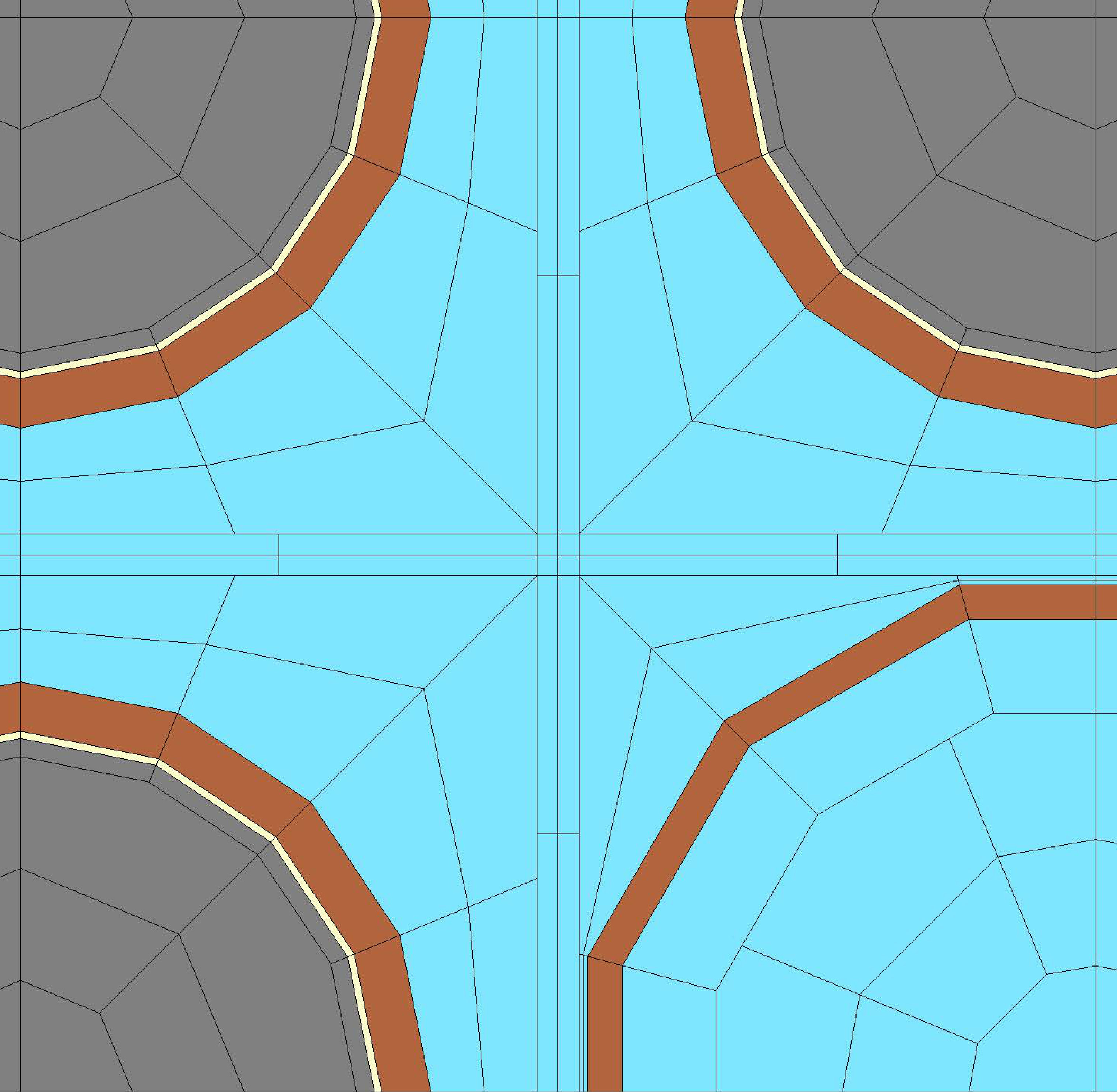 Figure 1
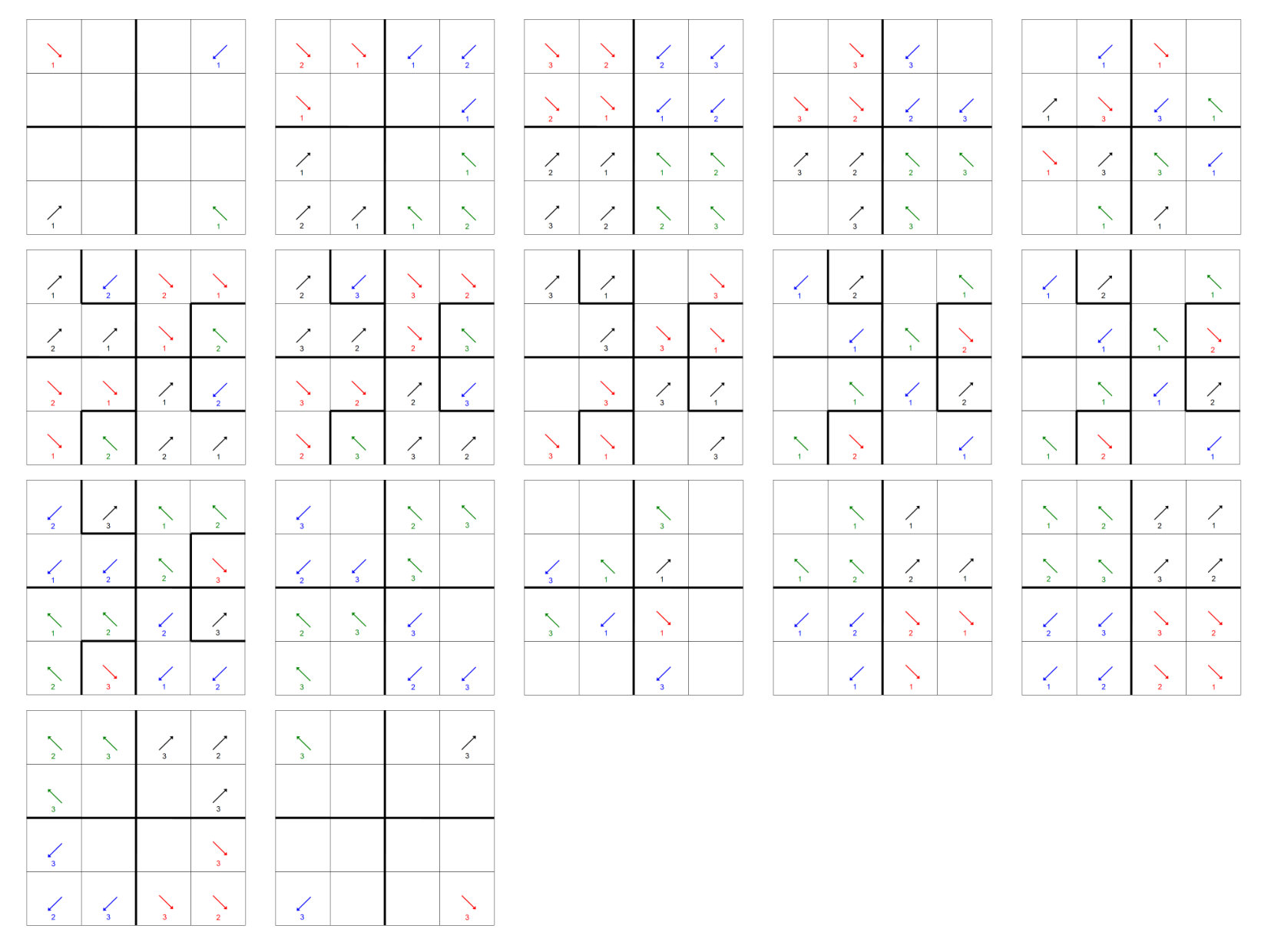 Figure 2
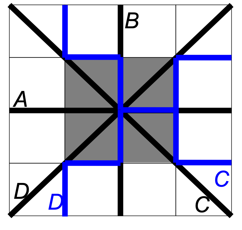 Figure 3
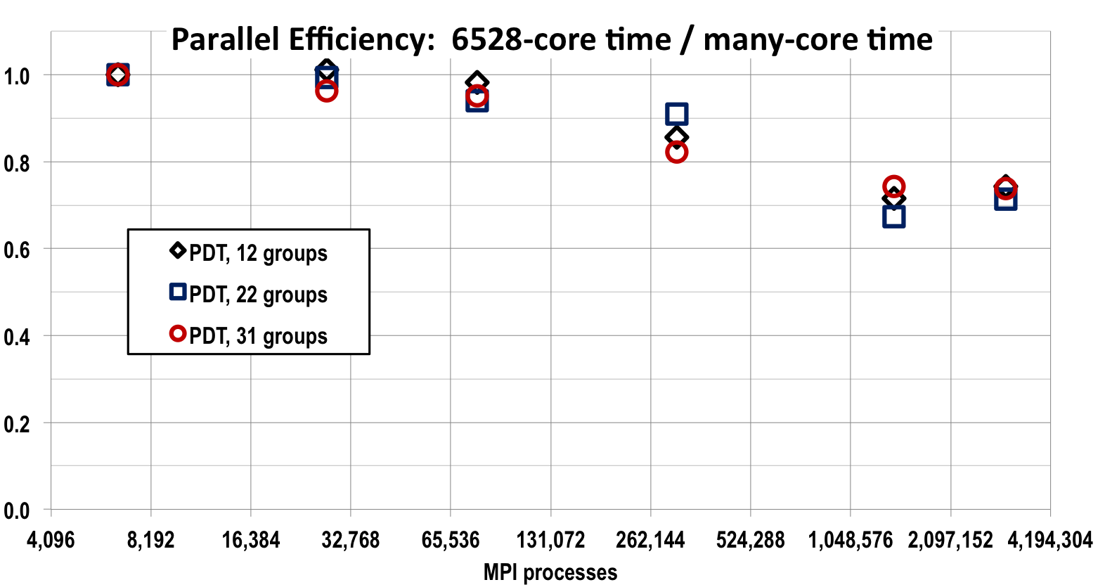 Figure 4
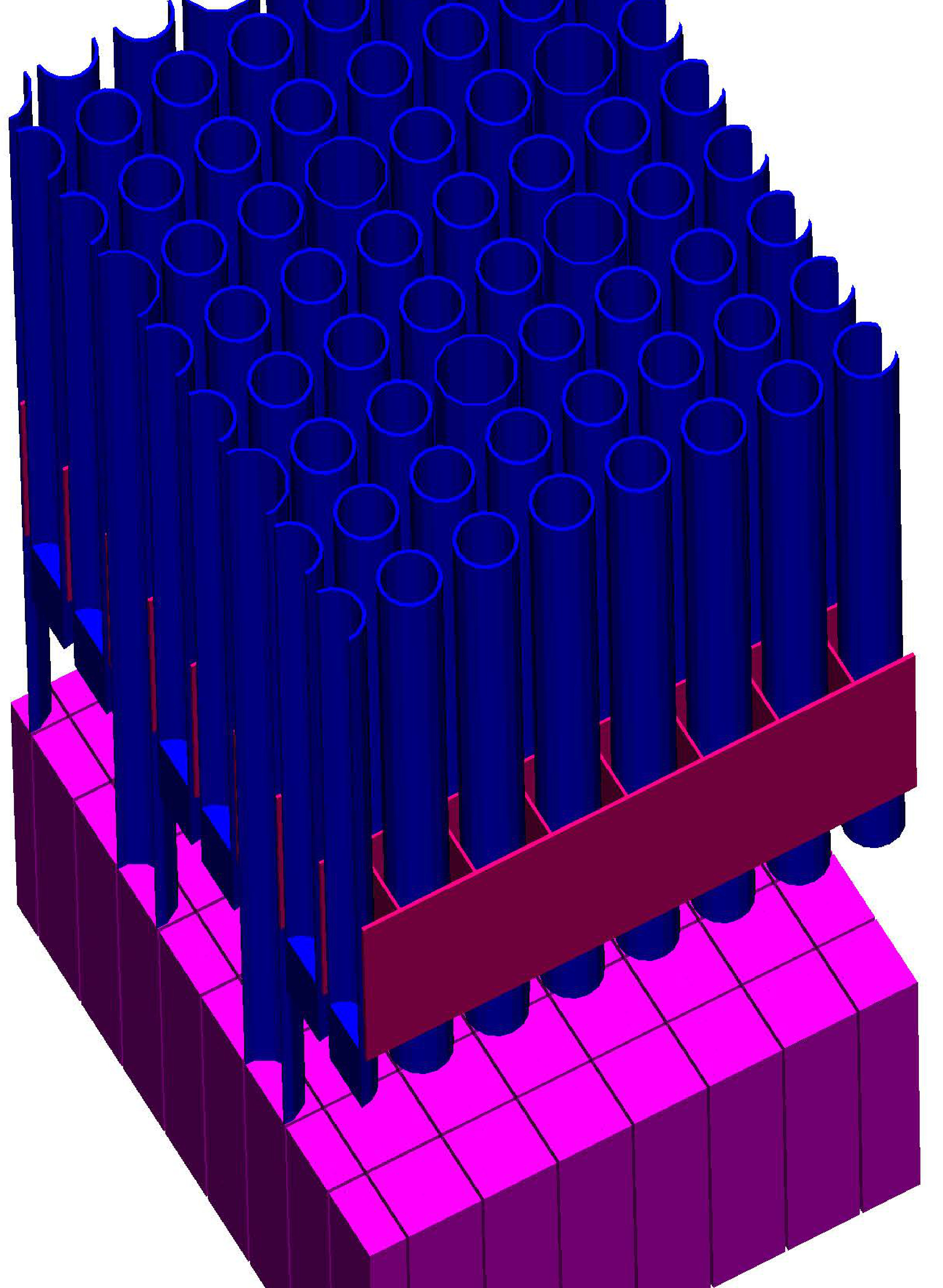 Figure 5
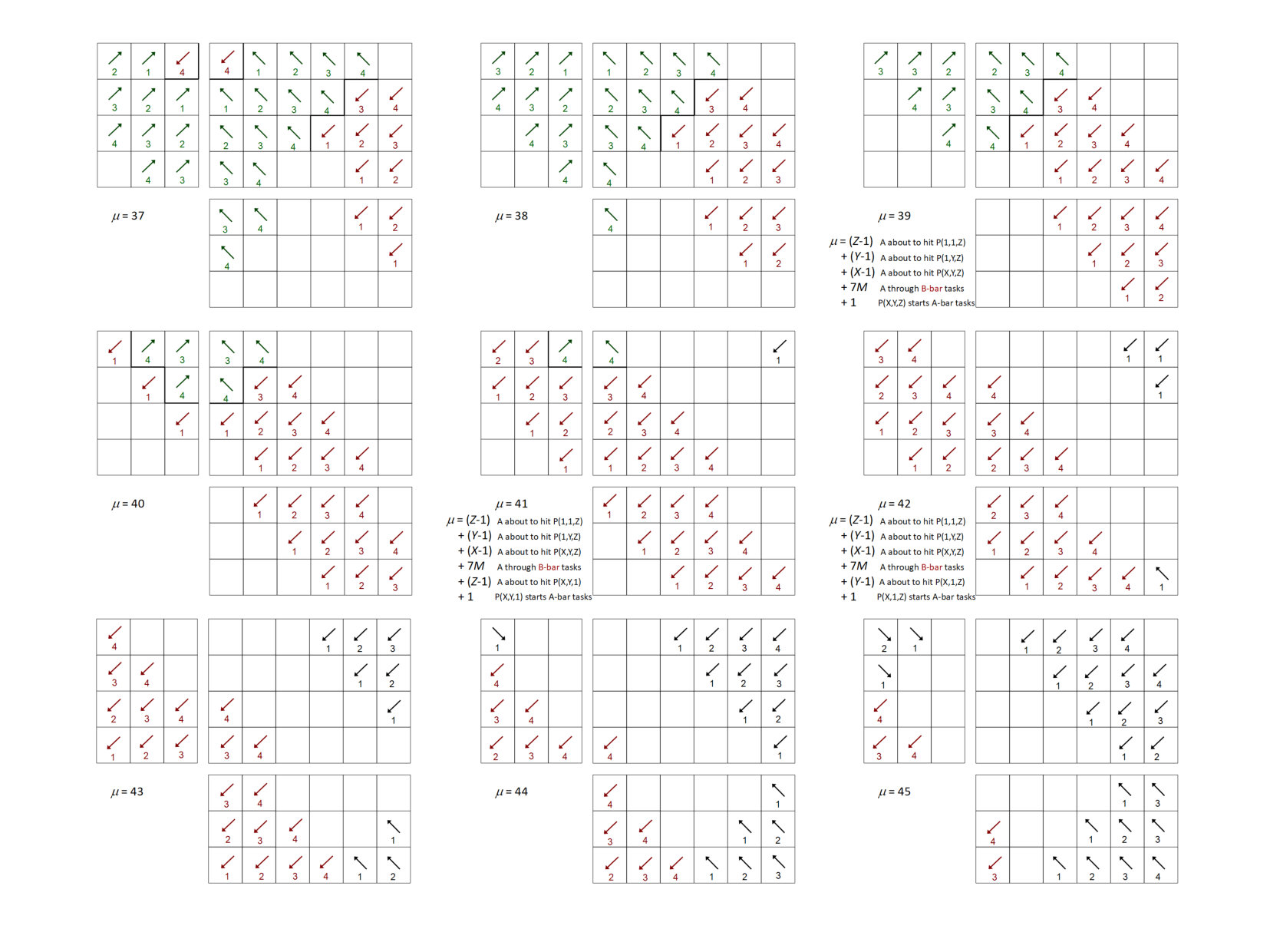 Figure 6
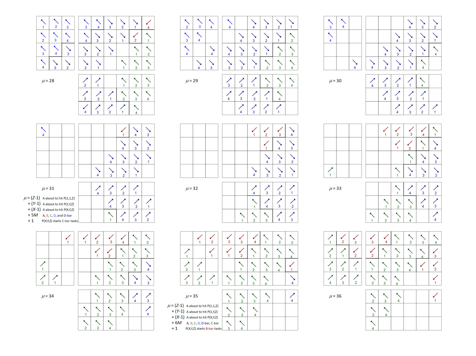 Figure 7
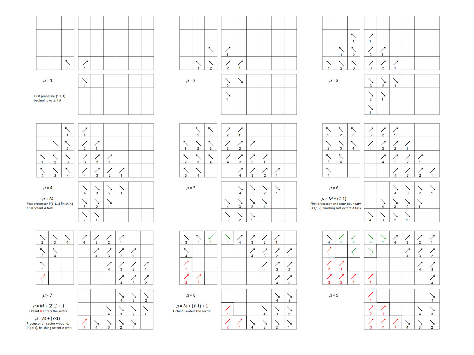 Figure 8
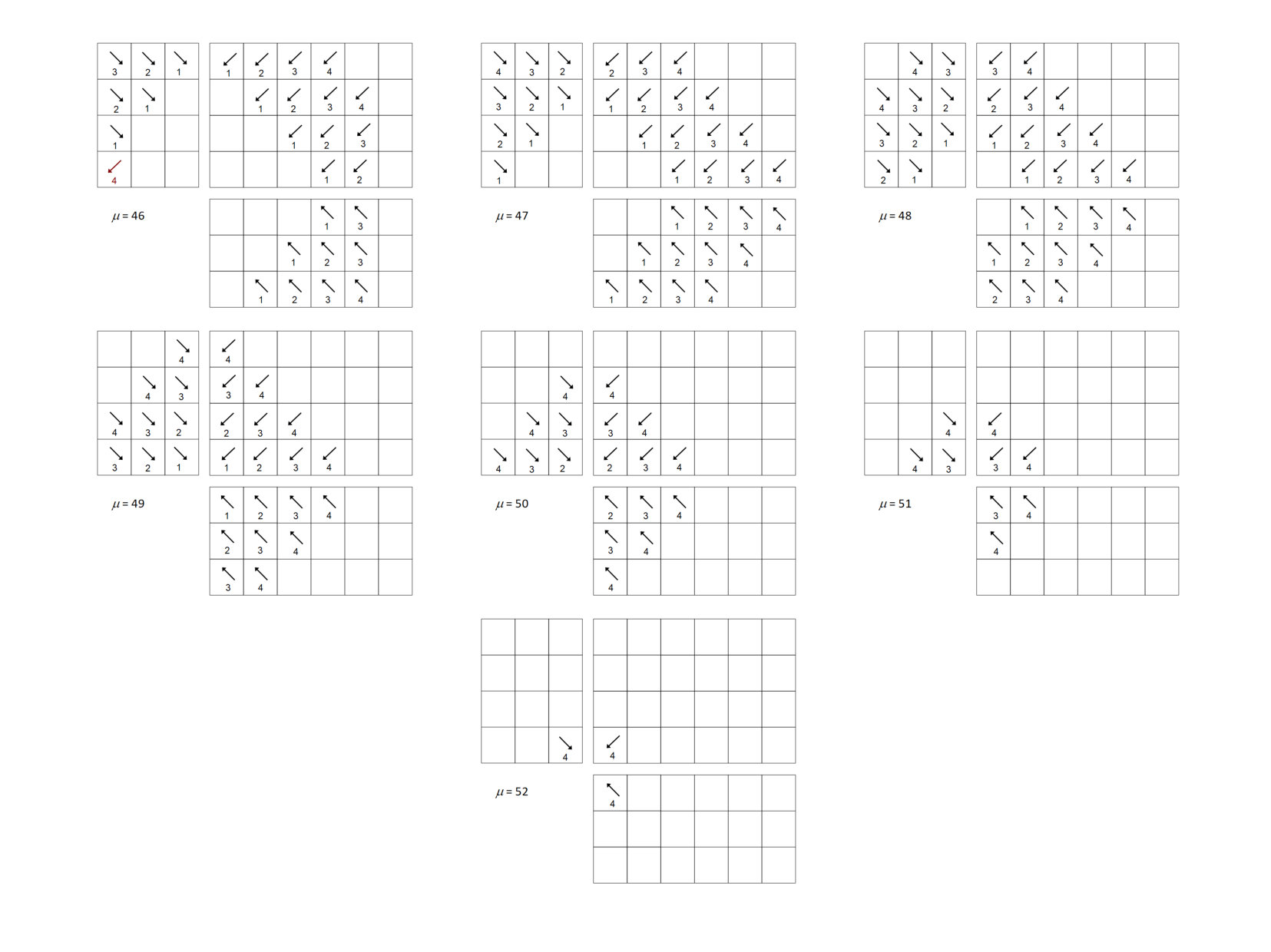 Figure 9
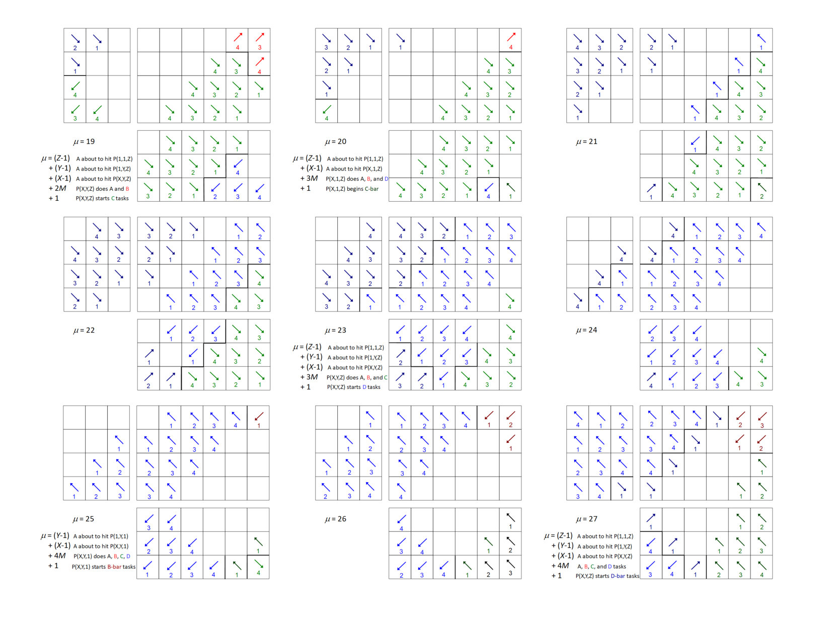 Figure 10
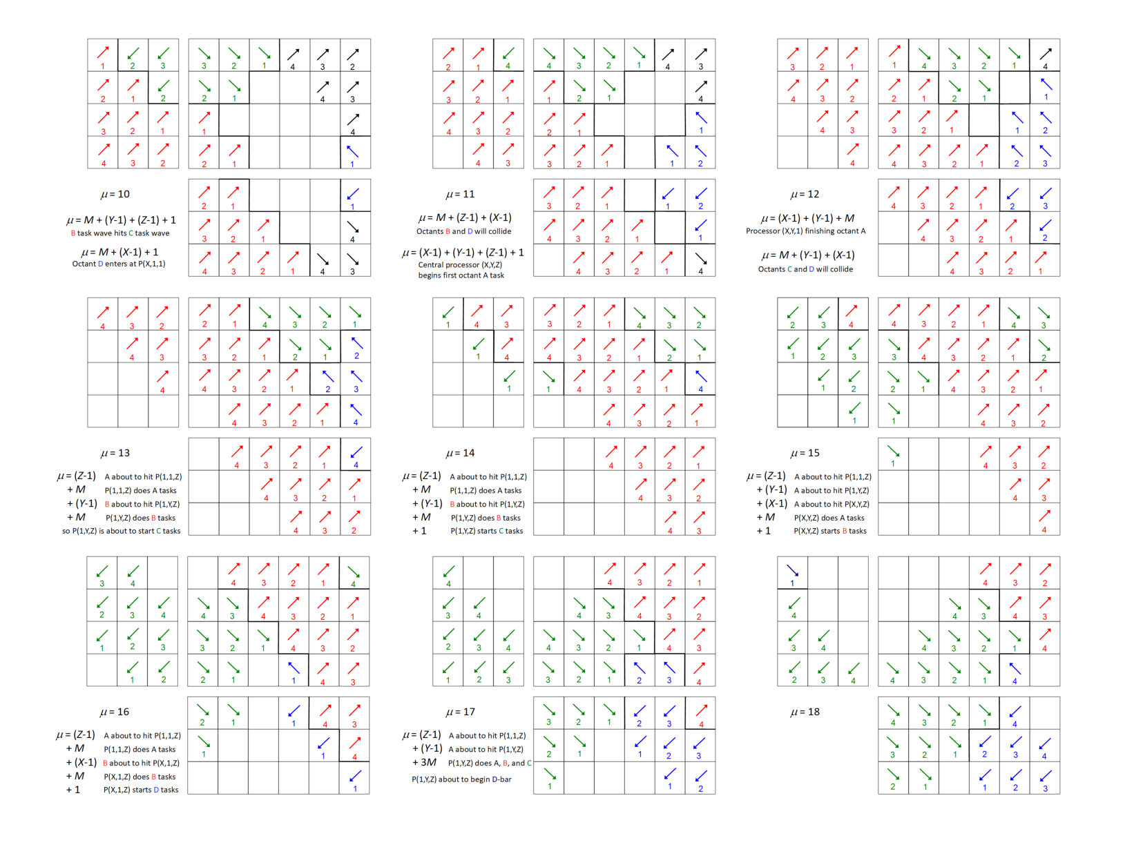 Figure 11
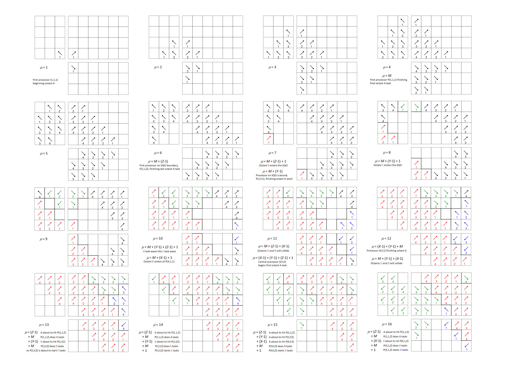 Figure 12
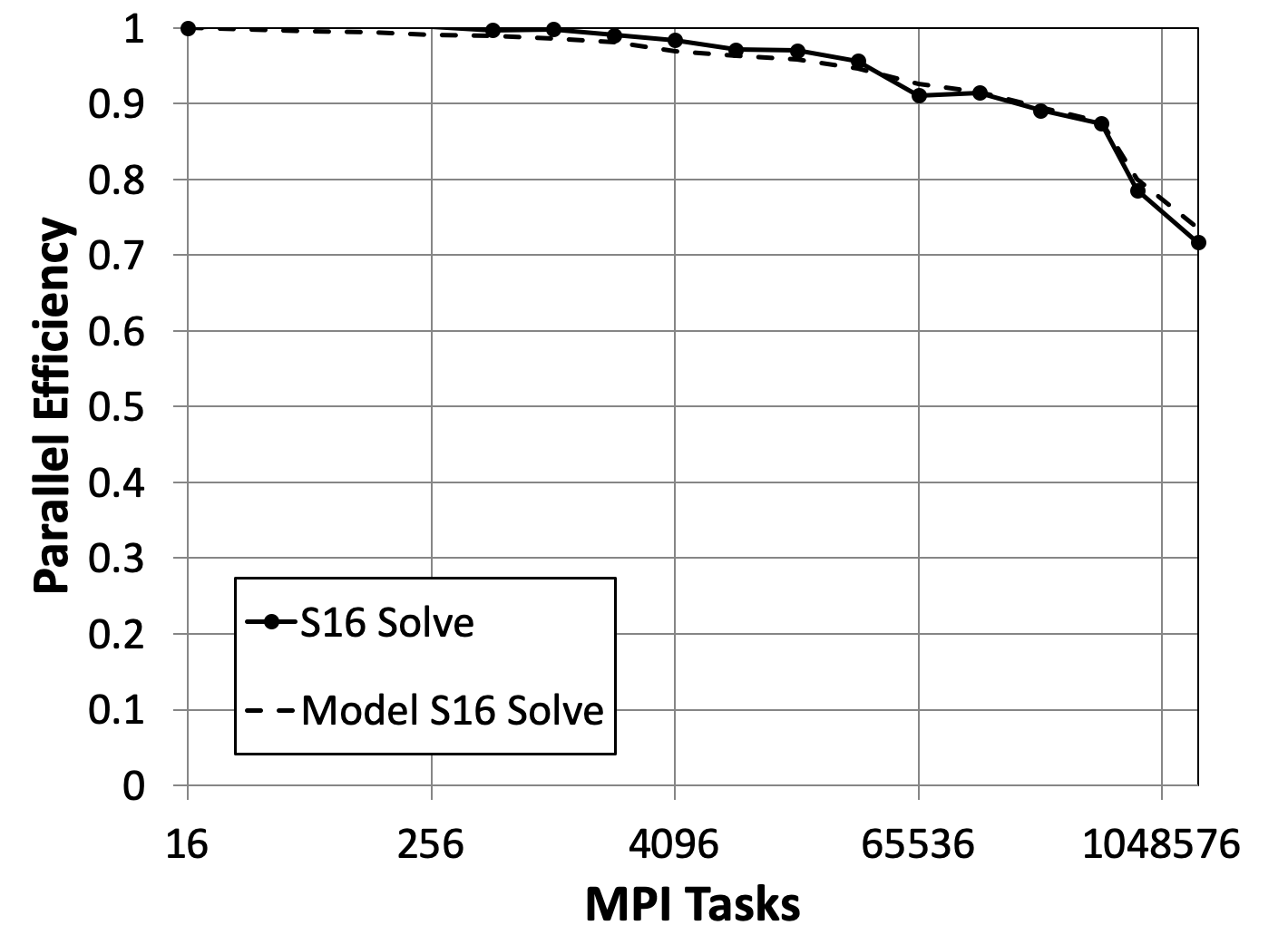 Figure 13
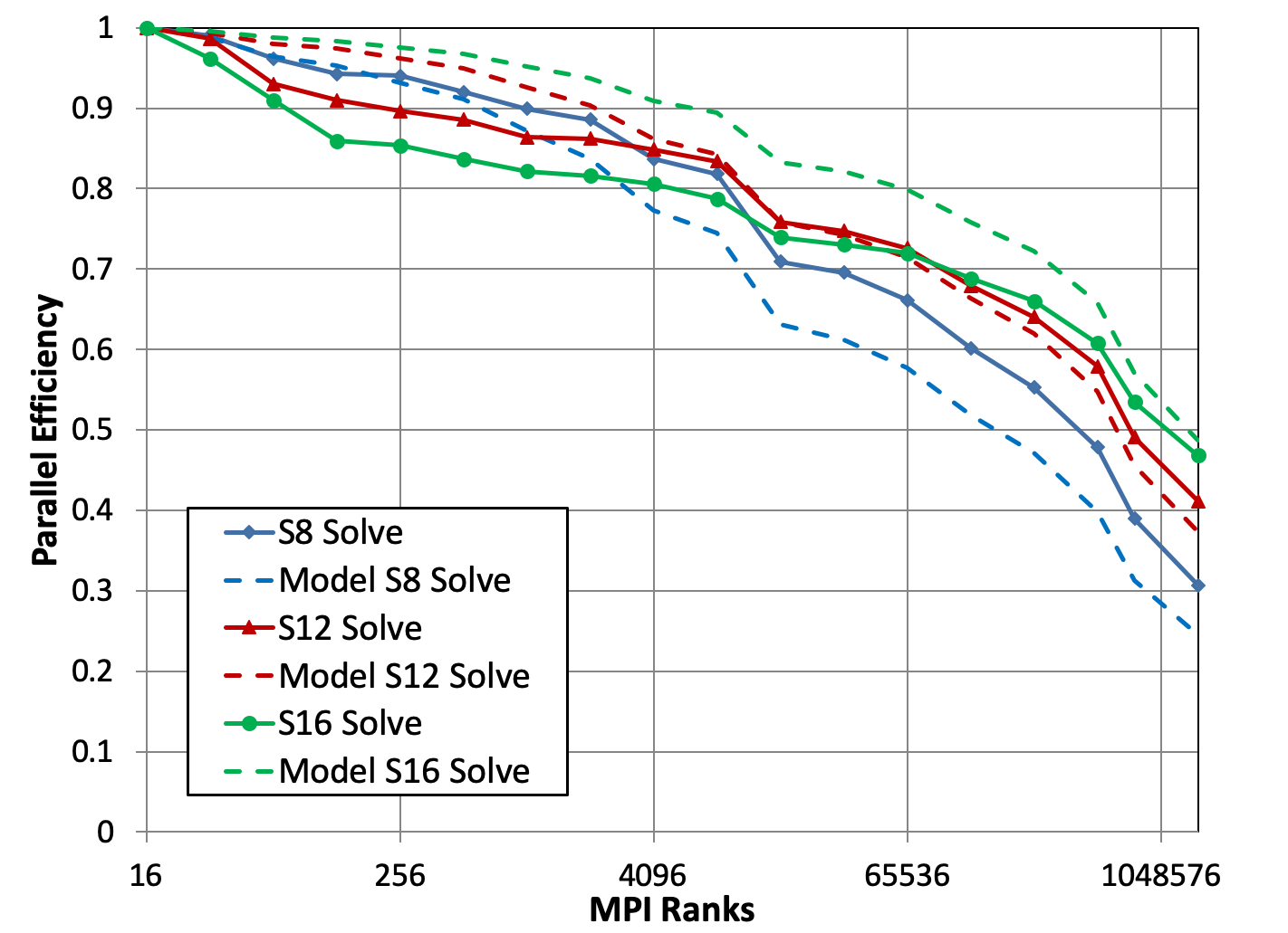 Figure 14
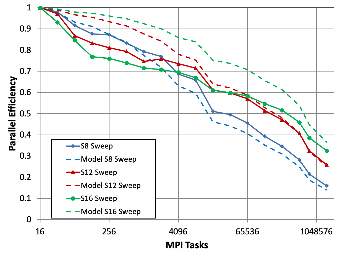 Figure 15
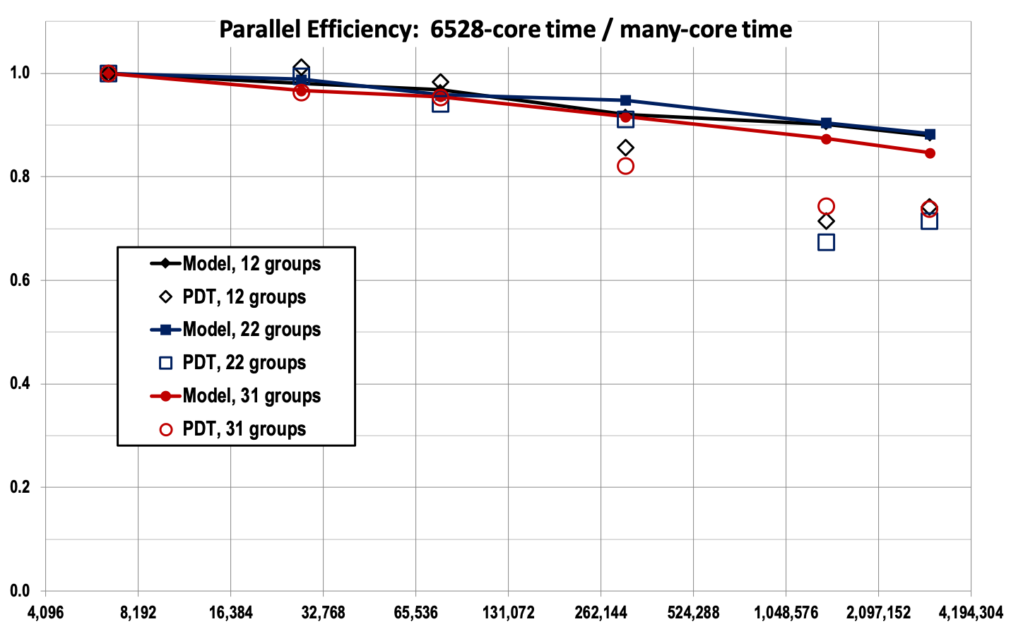 Figure 16
 Figure 17
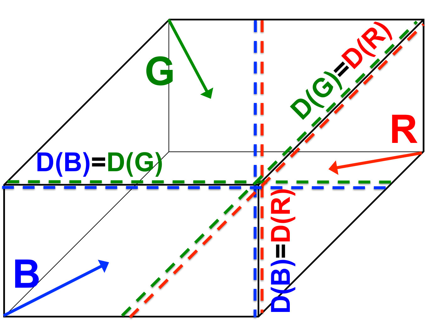 Figure 18
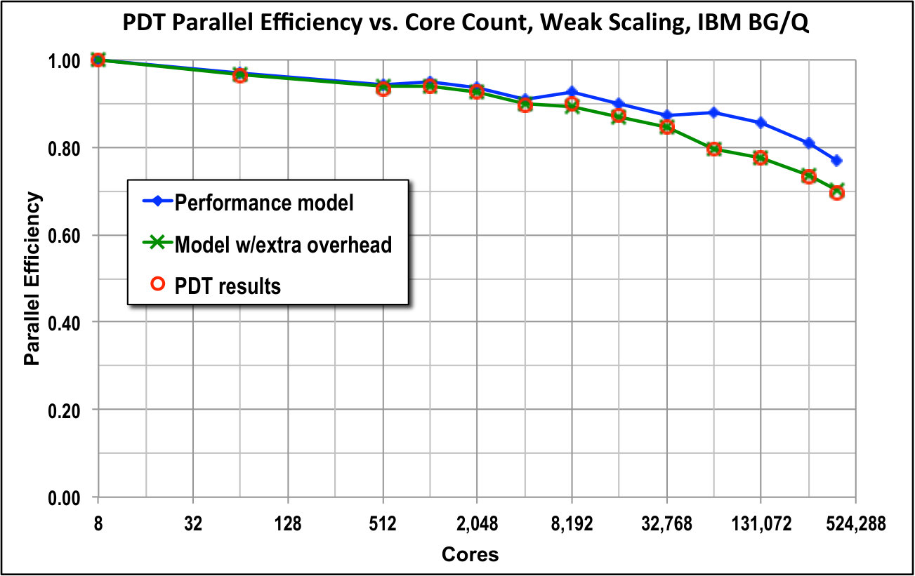 Figure 19
 Figure 1
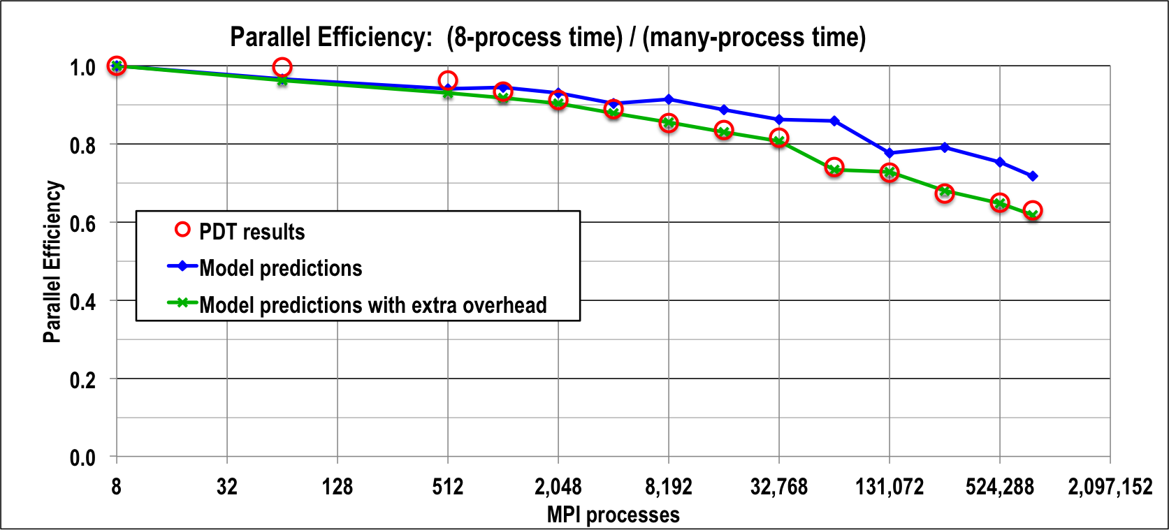 Figure 21
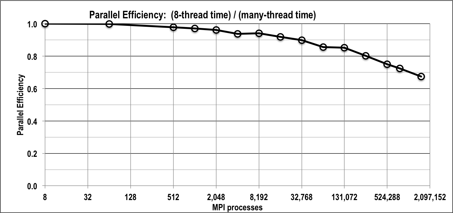 Figure 22
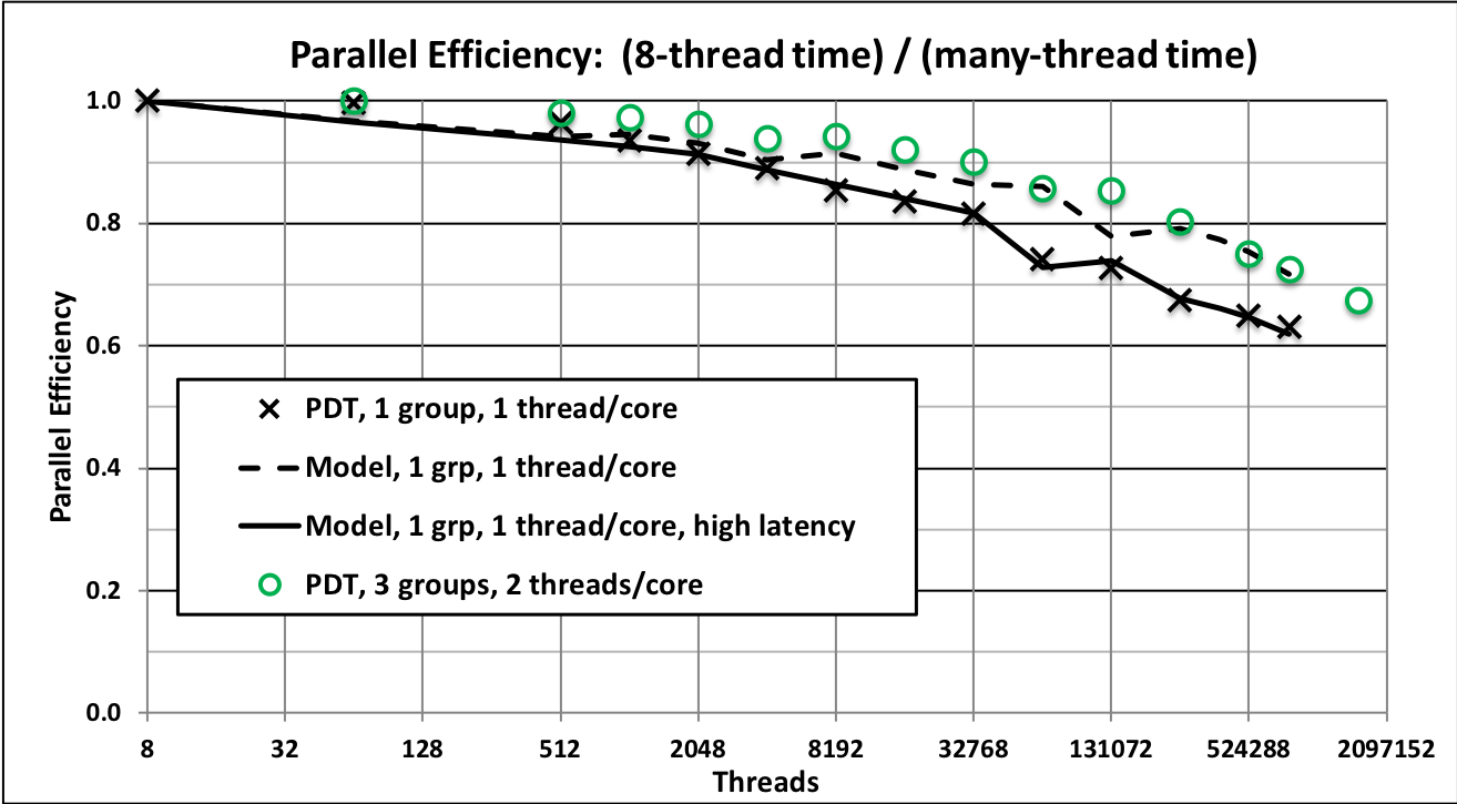 Figure 23
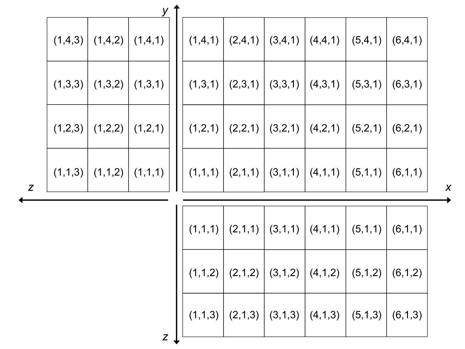 Figure 24
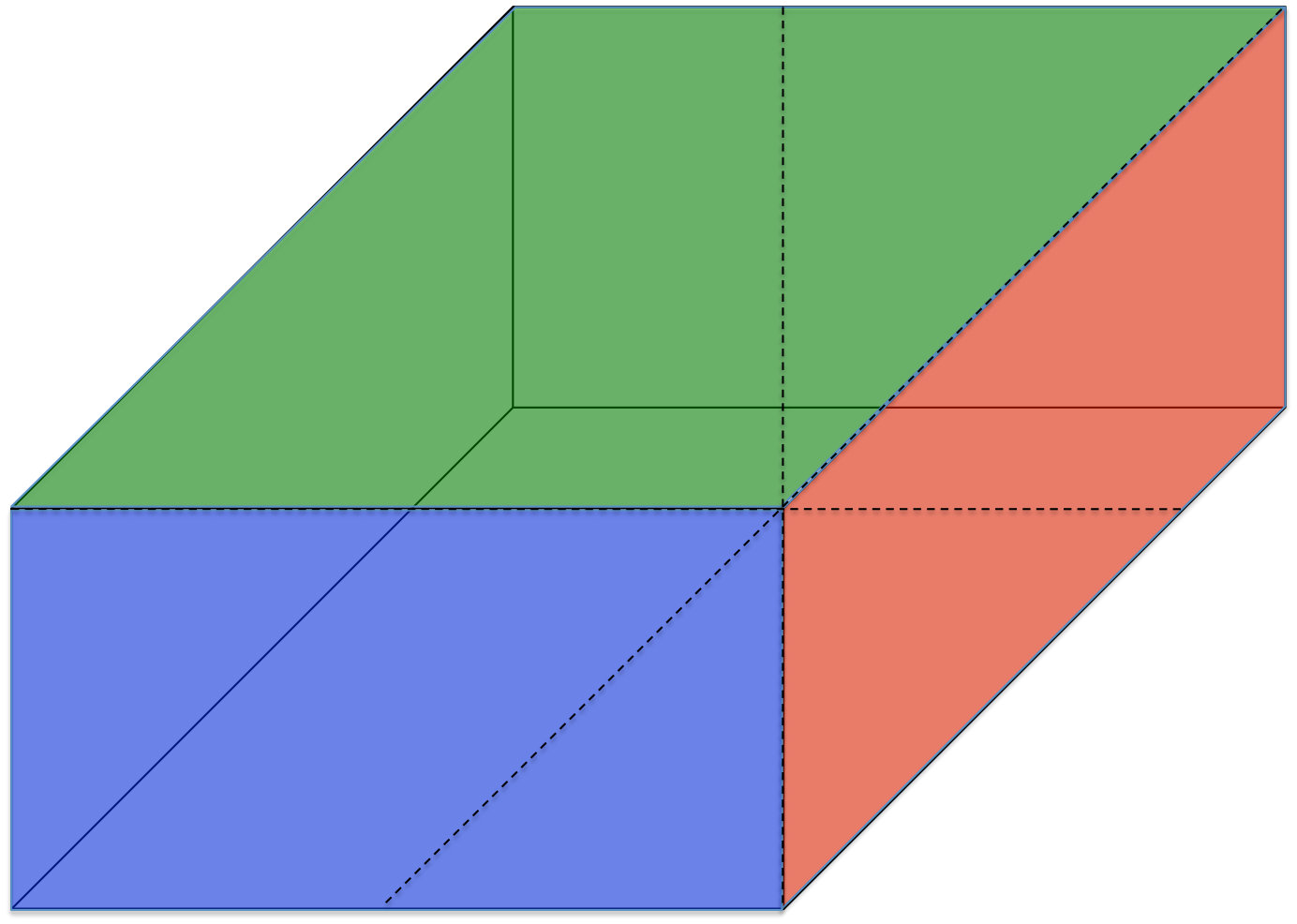 Figure 25
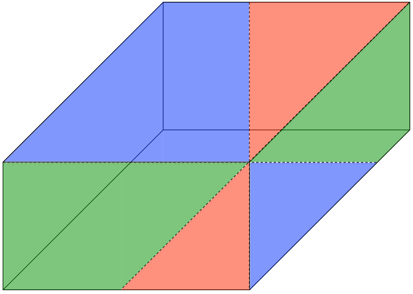 Figure 26
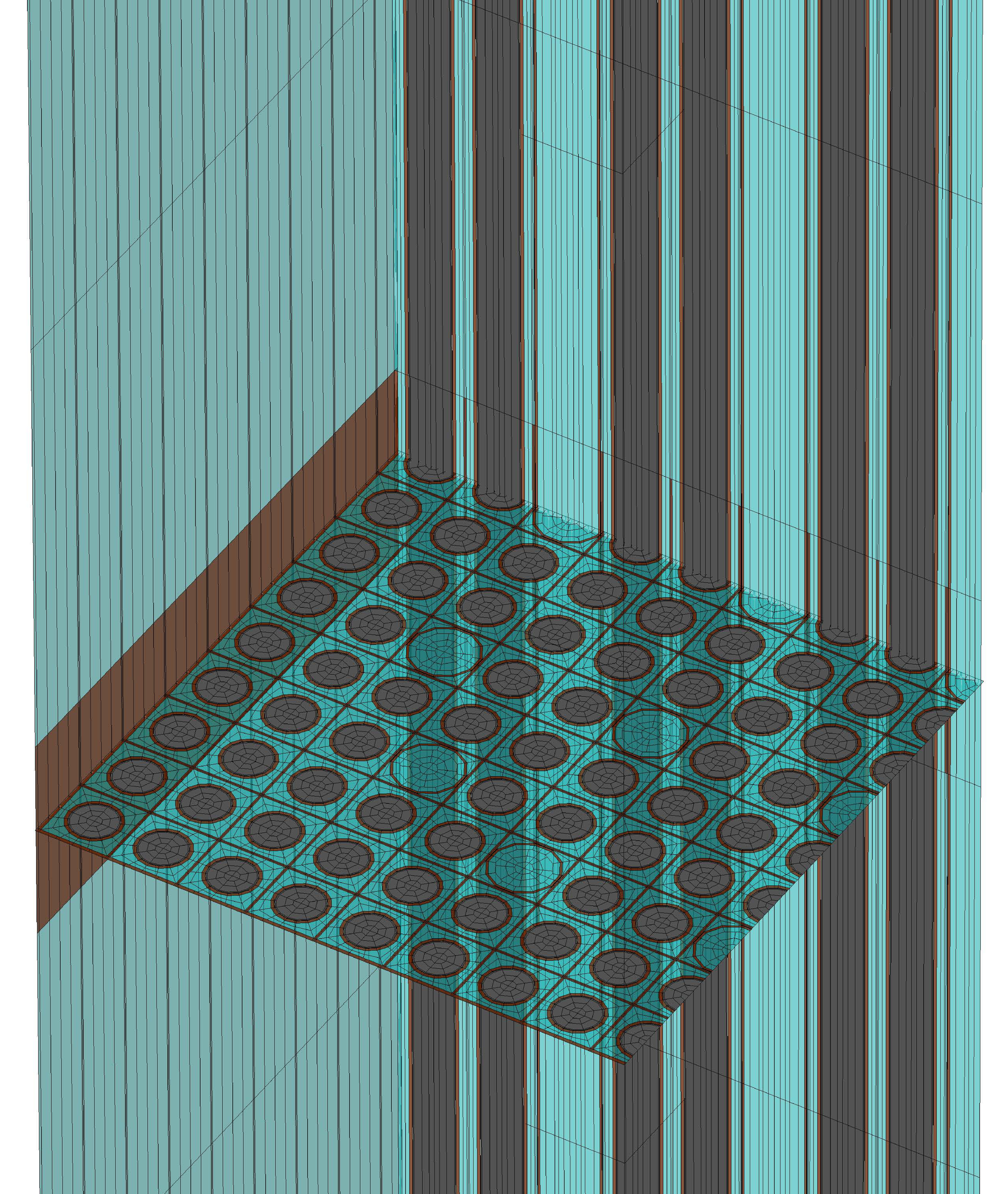 Figure 27
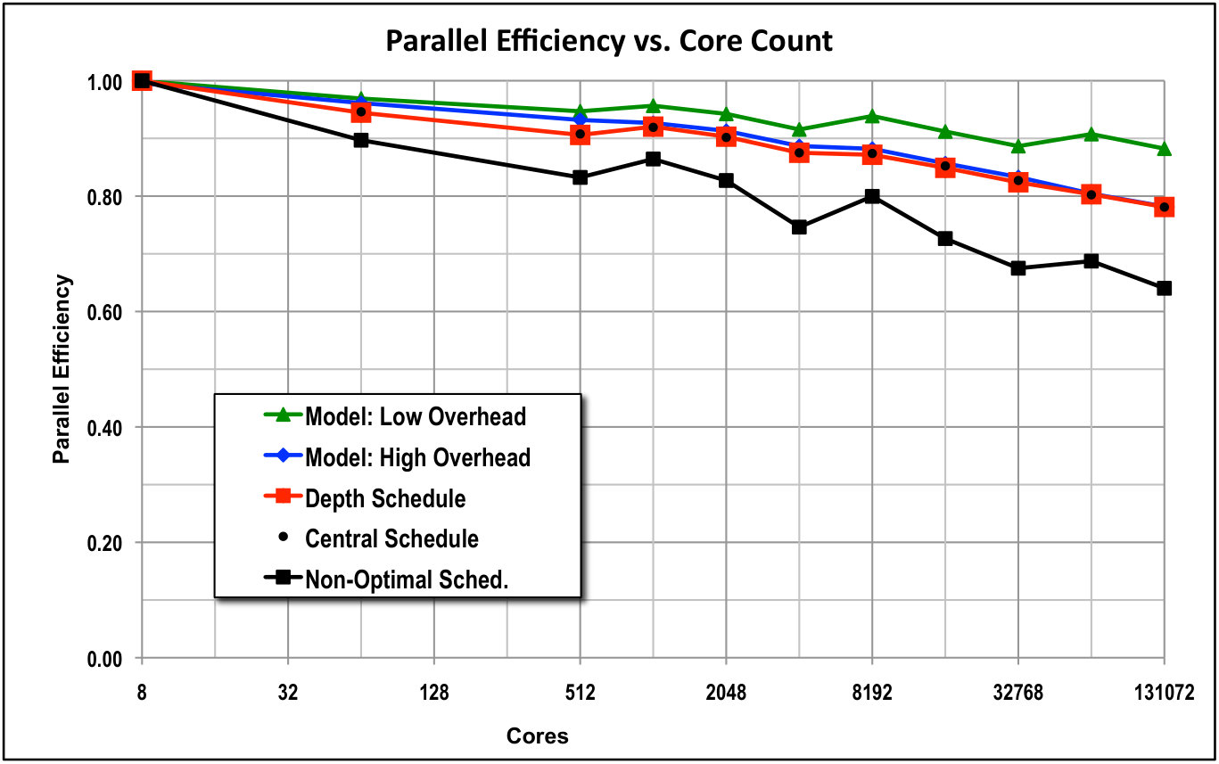 Figure 28
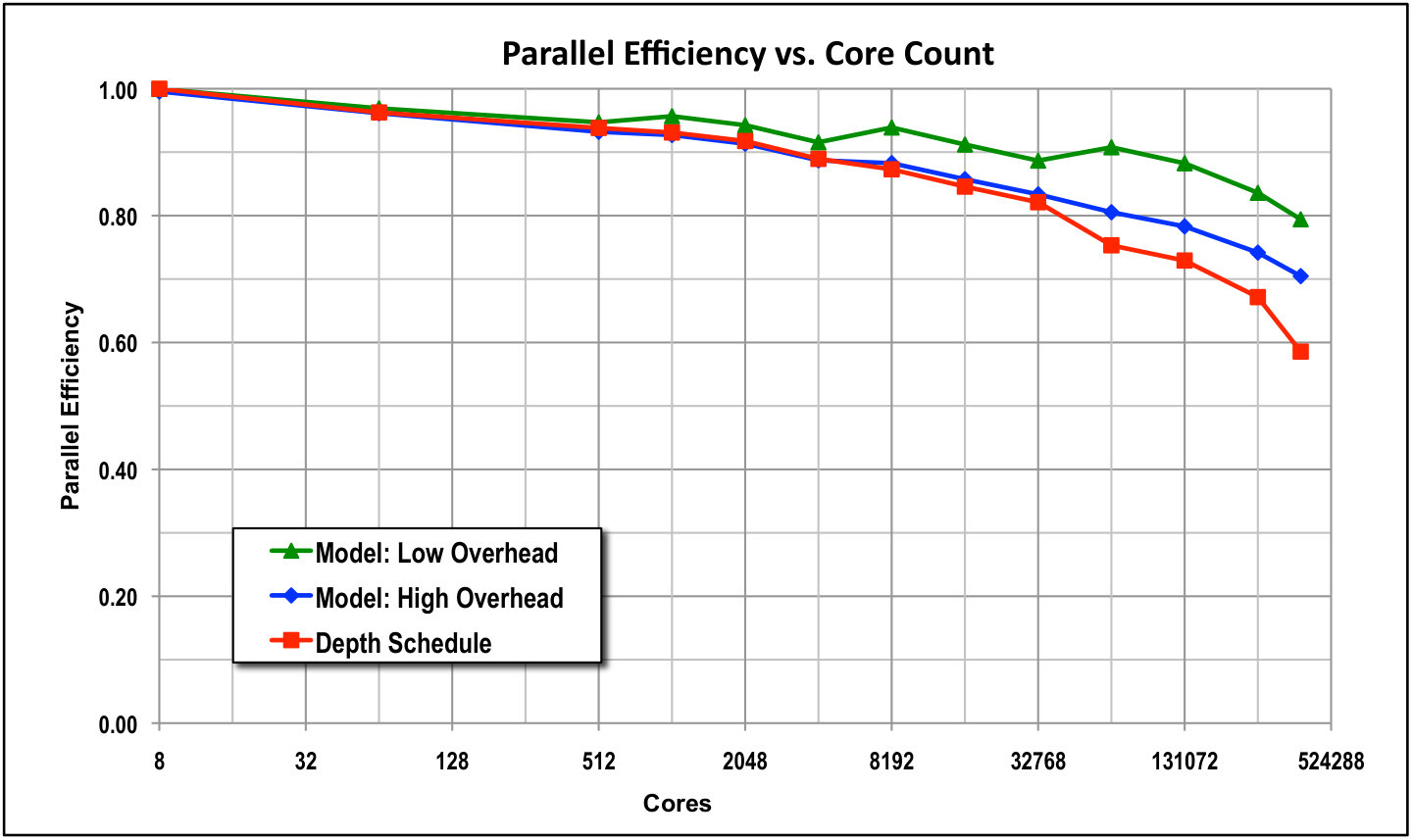 Figure 29
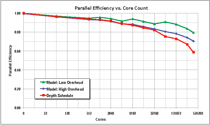 Figure 30
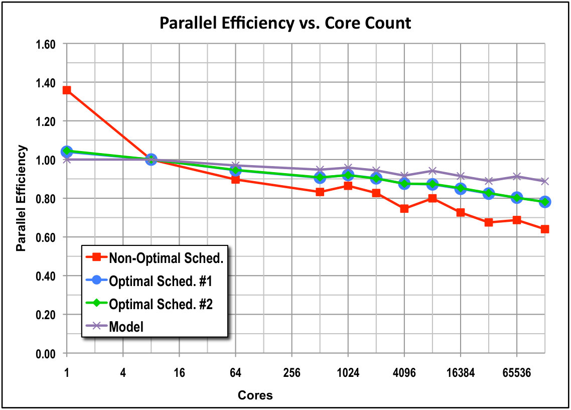 Figure 31
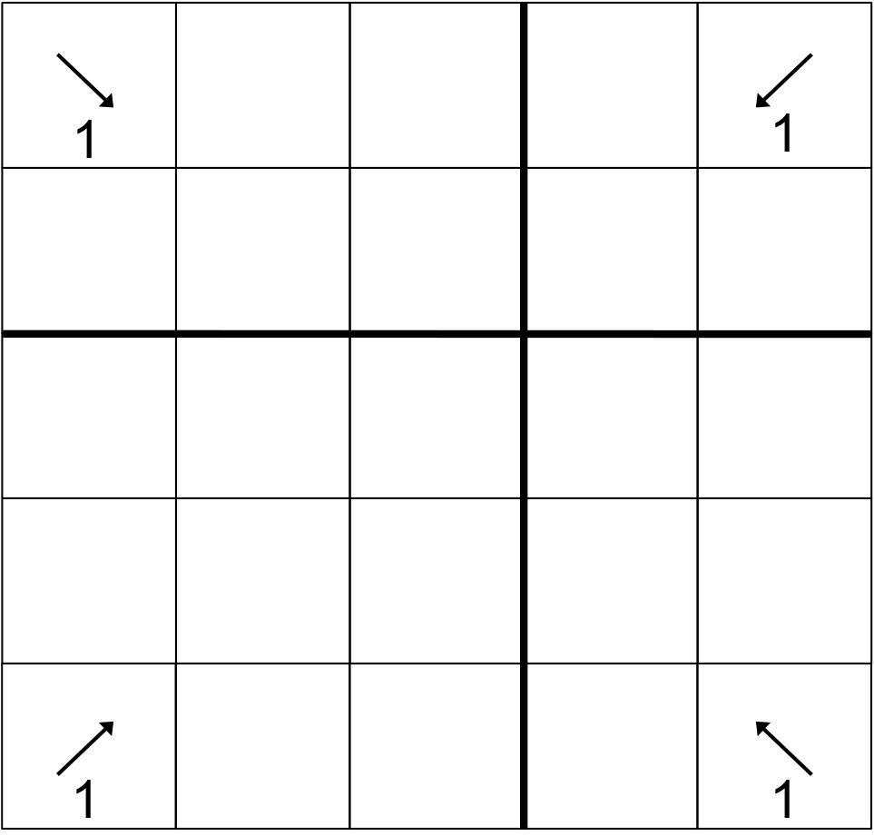 Figure 32
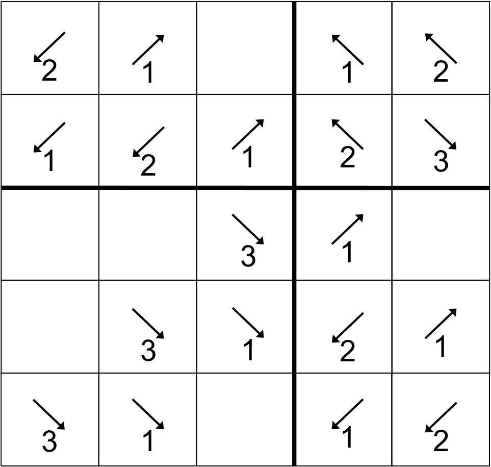 Figure 33
 Figure 34
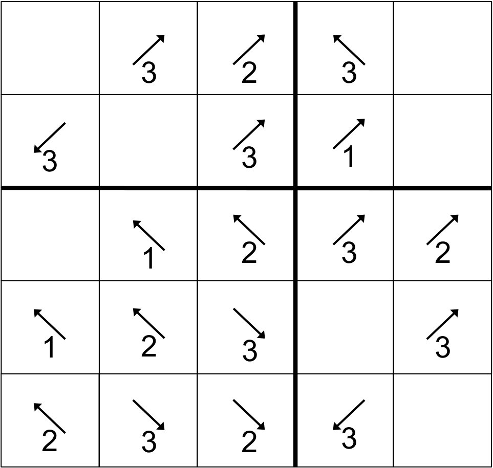 Figure 35
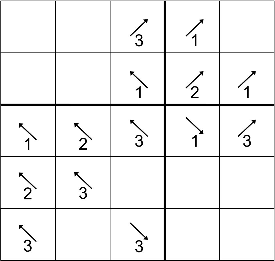 Figure 36
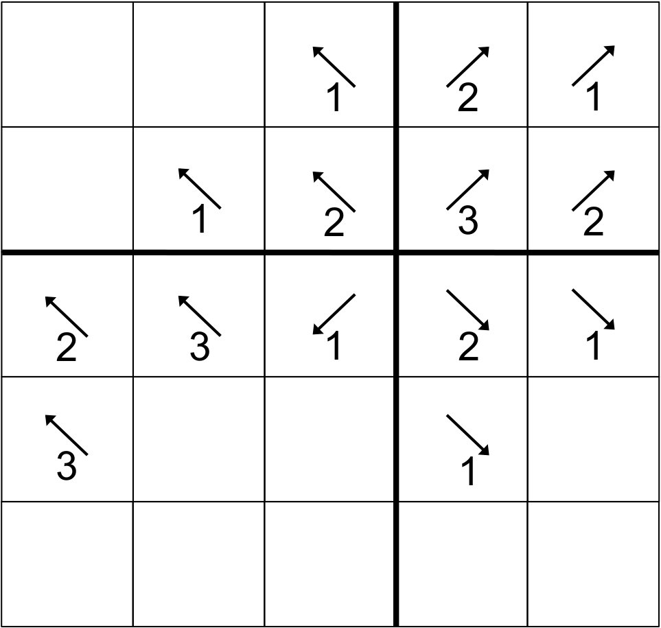 Figure 37
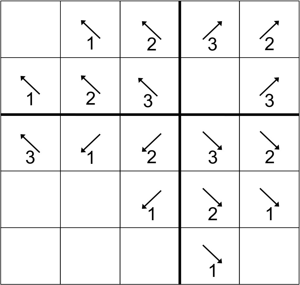 Figure 38
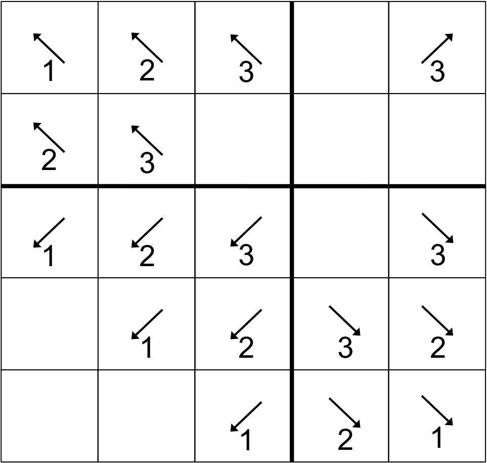 Figure 39
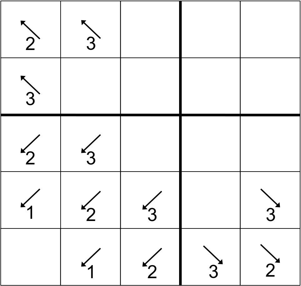 Figure 40
| Axial | Total | GS 1 | GS 2 | GS 3 | Total | ||
| Cores | Assys | cells | cells | (12 grps) | (31 grps) | (22 grps) | unknowns |
| directions | directions | directions | /core | ||||
| 6528 | 11 | 96 | 3.3 E6 | 8632 | 8616 | 888 | 2.3 E8 |
| 27,744 | 22 | 96 | 13.3 E6 | 8632 | 8616 | 8128 | 2.4 E8 |
| 78,608 | 22 | 136 | 1.9 E7 | 81232 | 81216 | 81212 | 2.2 E8 |
| 314,432 | 44 | 136 | 7.6 E7 | 81232 | 81216 | 81216 | 2.4 E8 |
| 1,414,944 | 66 | 136 | 1.7 E8 | 81648 | 81224 | 82416 | 2.1 E8 |
| 3,070,336 | 88 | 166 | 3.7 E8 | 81648 | 81224 | 82416 | 2.1 E8 |
Peer Reviews
No public reviews on file for this paper yet. If you reviewed it on a platform where reviews are public (OpenReview, ICLR, NeurIPS, ICML), you can paste yours below so the community can read it here.
Videos
No videos yet. Explain this paper in a talk, walkthrough, or lecture? Add one.
**PROVABLY OPTIMAL PARALLEL TRANSPORT SWEEPS ON SEMI-STRUCTURED GRIDS
**
**Michael P. Adams1, Marvin L. Adams1, W. Daryl Hawkins1,
Timmie Smith2, Lawrence Rauchwerger2**
1Dept. of Nuclear Engineering; 2Dept. of Computer Science and Engineering
Texas A&M University, 3133 TAMU, College Station, TX 77843-3133
{mpadams, mladams, dhawkins}@tamu.edu, [email protected], [email protected]
**Nancy M. Amato
**Dept. of Computer Science, University of Illinois
**Teresa S. Bailey, Robert D. Falgout, Adam Kunen, Peter Brown
**Lawrence Livermore National Laboratory
[email protected]; [email protected]; [email protected], [email protected]
ABSTRACT
We have found provably optimal algorithms for full-domain discrete-ordinate transport sweeps on a class of grids in 2D and 3D Cartesian geometry that are regular at a coarse level but arbitrary within the coarse blocks. We describe these algorithms and show that they always execute the full eight-octant (or four-quadrant if 2D) sweep in the minimum possible number of stages for a given partitioning. Computational results confirm that our optimal scheduling algorithms execute sweeps in the minimum possible stage count. Observed parallel efficiencies agree well with our performance model. Our PDT transport code has achieved approximately parallel efficiency with parallel threads, relative to 8 threads, on a simple weak-scaling problem with only three energy groups, 10 direction per octant, and 4096 cells/core. We demonstrate similar efficiencies on a much more realistic set of nuclear-reactor test problems, with unstructured meshes that resolve fine geometric details. These results demonstrate that discrete-ordinates transport sweeps can be executed with high efficiency using more than parallel processes.
Key Words: transport sweeps, parallel transport, parallel algorithms, PDT, STAPL, performance models, unstructured mesh
1 INTRODUCTION
Deterministic particle-transport methods approximate the particle angular flux (or density or intensity) in a multidimensional phase space as a function of time. The independent variables that define the solution phase space are position (3 variables), energy (1), and direction (2). The most widely used discretizations in energy are multigroup methods, in which the solution is calculated for discrete energy “groups.” The most common directional discretizations are discrete-ordinates methods, in which the solution is calculated only for specific directions. In the most widely used methods, the solution for a given spatial cell, energy group, and direction depends only on:
- the total volumetric source within the cell, and 2) the angular flux for that group and direction that is incident upon the cell surface. Each incident flux is the outgoing flux from an adjacent “upstream” cell or is given by boundary conditions.
To solve the transport equation for the full spatial domain, for a given collection of energy groups, and for a single direction, one approach is to start with the cell (or cells) whose incident fluxes for that direction are all provided by boundary conditions. (For any direction from a typical quadrature set and a rectangular spatial domain, this would be one cell at one corner of the domain.) Once the solution is found for this cell, its outgoing fluxes complete the dependencies for its downstream neighbors, whose solutions may then be computed. Their outgoing fluxes satisfy their downstream neighbors’ dependencies, etc., so each set of cells that gets completed readies another set, and the computation “sweeps” across the entire domain in the direction being solved. Performing this process for the full set of cells and directions is called a transport sweep.
The full-domain boundary-to-boundary sweep, in which all angular fluxes in a set of energy groups are calculated given previous-iterate values for the volumetric fixed-plus-collisional source, forms the foundation for many iterative methods that have desirable properties [1]. One such property is that iteration counts do not change with mesh refinement and thus do not grow as resolution is increased in a given physical problem—an important consideration for the high-resolution transport problems that require efficient massively parallel computing. A transport sweep calculates via the numerical solution of:
[TABLE]
where includes the collisional source evaluated using fluxes from a previous iterate or guess (denoted by superscript ). We emphasize that this is a complete boundary-to-boundary sweep of all directions, respecting all upstream/downstream dependencies, with no iteration on interface angular fluxes.
The parallel execution of a sweep is complicated by the dependencies of cells on upstream neighbors. A task dependence graph (TDG) for one direction in a 2D example (Figs. 1a and b) illustrates the issue: tasks at a given level of the graph cannot be executed until some tasks finish on the previous level. This originally led to a widespread perception that parallel sweeps cannot be efficient beyond a few thousand parallel processes and provided motivation for researchers to seek iterative methods that do not use full-domain sweeps [2, 3]. Such methods offer the possibility of easier scaling to high process counts—for a single iteration’s calculation—but iteration counts may increase as each process’s physical subdomain size decreases, which tends to happen as resolution and process count both increase.
In this paper we focus on discrete-ordinates transport sweeps and describe new parallel sweep algorithms. We demonstrate via theory, models, and computational results that our new provably optimal sweep algorithms enable efficient parallel sweeps out to O() parallel processes, even with modest problem sizes ((1M) cell-energy-direction elements per process). We describe a framework for understanding and exploiting the available concurrency in a sweep, recognizing that fundamental dependencies prevent sweeps from being “embarrassingly parallel.” We discuss and integrate algorithmic features from past research efforts, providing a comprehensive view of the trade-space available for sweep optimization [6, 7, 8, 9, 10].
The key components of a sweep algorithm are partitioning (dividing the domain among processes), aggregation (grouping cells, directions, and energy groups into “tasks”), and scheduling (choosing which task to execute if more than one is available). The KBA algorithm devised by Koch, Baker, and Alcouffe [6] and the algorithm by Compton and Clouse [8] exploit parallel concurrency enabled by particular partitioning and aggregation choices. We generalize this as follows. Given a grid with spatial cells, let us aggregate cells in to brick-shaped cellsets in a array. We then distribute these cellsets across processes, with the possibility of assigning more than one cellset to each process. This corresponds to “blocks” in KBA and spatial domain “overloading” in other work [8, 10]. It is possible to also distribute energy groups and/or quadrature directions across different processes, but in this work we focus on spatial decomposition.
In this paper we limit our analysis to “semi-structured” spatial meshes that can be unstructured at a fine level but are orthogonal at a coarse level, allowing for aggregation into a regular grid of brick-shaped cellsets. Fully irregular grids introduce complications that we will not address in this paper. We assume spatial domain decomposition in which each process owns a contiguous brick-shaped subdomain. In a future communication we expect to address decompositions in which a process may own non-contiguous portions of the spatial domain [4]. In the analysis of sweep optimality presented below, we assume load-balanced cellsets, with each cellset containing the same number of cells with the same number of spatial degrees of freedom. The work presented here is based on a recent conference paper [5] but is augmented to include: 1) an extension of our optimal-sweep algorithm to reflecting boundaries, 2) an improved performance model, 3) updated and extended numerical results, and 4) a relaxation of constraints on spatial meshes.
The KBA algorithm devised by Koch, Baker, and Alcouffe [6] is the most widely known parallel sweep algorithm. KBA partitions the problem by assigning a column of cells to each process, indicated by the four diagonal task groupings in Fig.1c. KBA parallelizes over planes logically perpendicular to the sweep direction—over the breadth of the TDG. Early and late in a single-direction sweep, some processes are idle, as in stages 1-3 and 9-11 in Fig.1. In this example, parallel efficiency for an isolated single-direction sweep could be no better than . KBA is much better, because when a process finishes its tasks for the first direction it begins its tasks for the next direction in the octant-pair that has the same sweep ordering. That is, each process begins a new TDG as soon as it completes its work on the previous TDG, until all directions in the octant-pair finish. This is equivalent to concatenating all of an octant-pair’s TDGs into a single much longer TDG. This lengthens the “pipe” and increases efficiency. If there were directions in the octant pair, then the pipe length is in this example, and the efficiency would be if communication times were negligible.
The scheduling algorithm described here is valid for any spatial grid of cells that can be aggregated into brick-shaped cellsets. A familiar example of a non-orthogonal grid with this property is a reactor lattice. As the term “lattice” implies, these grids are regular at a coarse level despite being unstructured at the cell level. Additionally, an unstructured mesh that is “cut” along full-domain planes can employ the algorithm described here. As we describe below, prismatic grids that are extrusions of 2D meshes into cell-planes—such as those commonly found in 3D nuclear-reactor analysis—offer advantages in optimizing sweeps, but extruded grids are not required by our algorithm.
The coarse regularity of brick-shaped cellsets allows us to partition the domain into a process grid, with number of processes . The work to be performed in the sweep is to calculate the angular intensity for each of the directions in each of the energy groups in each of the spatial cells, for a total of fine-grained work units. The finest-grained work unit is calculation of a single direction and energy group’s unknowns in a single cell; thus, we describe the sweeps that we analyze here as use “cell-based.” Methods based on solutions along characteristics permit finer granularity of the computation; in particular, “face-based” sweeps are possible, and with long-characteristic methods “track-based” sweeps are possible. Face-based and track-based sweeps offer advantages over cell-based sweeps in terms of potential parallel efficiency, but in this paper we focus on cell-based sweeps.
We aggregate fine-grained work units into coarser-grained tasks, with each task being the solution of the angular fluxes in groups, directions, and spatial cells. (The s are “aggregation factors.”) Since our scheduling algorithm is based on brick cellsets, is constrained by the level of regularity in the grid. We use the term “cell subset” to refer to the smallest orthogonal units of the mesh, which we can combine into cellsets as we see fit. Thus, if our grid is a lattice of brick subsets of cells, then will be an integer multiple of . Our choice of “subset aggregation factors” , , and determines our cellset layout, with each .
In order to maintain load balance, we require that each process in our partitioning scheme own the same number of cellsets . Here, is the spatial “overload factor”, and if it is greater than one we say that our partitioning and aggregation scheme is “overloaded”, since processes own multiple cellsets. This can be broken down as , with . As will be clear from the efficiency formulas in Sec. 2, there can be significant benefit from overloading. With everything partitioned and aggregated, each process is responsible for cellsets, group-sets, and direction-sets, for a total of tasks.
The directions that are aggregated together are required to be within the same octant. The sweep for directions in a given octant must begin at one of the eight corners of the spatial domain and proceed to the opposite corner. If direction-sets from multiple octants are launched at the same time, there will be “collisions” in which a process or set of processes will have multiple tasks available for execution. A scheduling algorithm is required for choosing which task to execute.
Scheduling algorithms are a primary focus of this paper. Our work builds on heuristics-based scheduling algorithms that previous researchers devised [8, 9, 10] to address the schedule conflicts that arise from launching simultaneous sweep fronts from all corners of the spatial domain. In this paper we introduce a family of scheduling algorithms that execute the complete 8-octant sweep in the minimum possible number of “stages,” where a stage is defined as execution of a single task (cellset/direction-set/groupset) and subsequent communication, by each process that has work available. We outline a proof of optimality for one member of the family, discuss the others, and present computational results, which demonstrate that our optimal scheduling algorithms do indeed complete their sweeps in the minimum possible number of stages and provide high efficiency even at high process counts.
With an optimal scheduling algorithm in hand we know how many stages a sweep will require. This is a simple function of the partitioning and aggregation parameters chosen for any given problem. With stage count known, there is a possibility of predicting execution time via a performance model, and then using the model to choose partitioning and aggregation factors that minimize execution time for the given problem on the given number of processes on the given machine. The result is what we call an “optimal sweep algorithm.” To recap, the ingredients of the optimal sweep algorithm are:
A sweep scheduling algorithm that executes in the minimum possible number of stages for a given problem with given partitioning and aggregation parameters; 2. 2.
A performance model that estimates execution time for a given problem as a function of stage count, machine parameters, partitioning, and aggregation; 3. 3.
An optimization algorithm that chooses the partitioning and aggregation parameters to minimize the model’s estimate of execution time.
In the following section we discuss and quantify key characteristics of parallel sweeps, including: 1) the idle stages that are inevitable if sweep dependencies are enforced, and 2) a lower bound on stage count. We also develop and discuss simple performance models. The third section describes our optimal scheduling algorithms, which achieve the lower-bound stage count found in Sec. 2. For one algorithm we prove optimality for three kinds of partitioning: (KBA partitioning), (“hybrid”), and (“volumetric”). (To simplify the discussion we define such that .) This is the first main contribution of this paper. In the fourth section we present our optimal sweep algorithm, which is made possible by our optimal scheduling algorithm. For optimal sweeps, we automate the selection of partitioning and aggregation parameters that minimize execution time, as predicted by our performance model, given the knowledge that sweeps will complete in the minimum possible number of stages for a given set of parameters. This is the second main contribution. Section 5 presents results ranging from 8 to approximately 1.5 million parallel processes, with two different optimal-scheduling algorithms and one non-optimal algorithm. In all cases the optimal algorithms complete the sweeps in the minimum possible number of stages, and performance agrees reasonably well with the predictions of our performance model. We offer summary observations, concluding remarks, and suggestions for future work in the final section. Appendices provide graphic illustrations of the behavior of optimally scheduled sweeps in 2D and 3D.
2 PARALLEL SWEEPS
Consider a process layout on a spatial grid of cells. Suppose there are directions per octant and energy groups that can be swept simultaneously. Then each process must perform cell-direction-group calculations. We aggregate these into tasks, with each task containing cells, directions, and groups. Then each process must perform tasks. At each stage at least one process computes a task and communicates to downstream neighbors. The complete sweep requires stages, where is the number of idle stages for each process. Parallel sweep efficiency (serial time per unknown / parallel time per unknown per process) is therefore approximately
[TABLE]
where is the time to compute one task and is the time to communicate after completing a task. In the second line, the term in the first [ ] is the idle-time penalty and the term in the second [ ] is the comm penalty. Aggregating into small tasks ( large) minimizes idle-time penalty but increases comm penalty: latency causes to increase as tasks become smaller. This assumes the most basic comm model, which can be refined to account for architectural realities (hierarchical networks, random variations, dedicated comm hardware, latency-hiding techniques, etc.).
In the terms defined above we describe “basic” KBA as having , (), (), , , and selectable number of -planes to be aggregated into each task. (A variant described in the original KBA paper is to aggregate directions by octant, which means and .) In our language, and translate to . With , or 8, and , each process performs tasks. With basic KBA, then, tasks (two octants) are pipelined from a given corner of the 2D process layout in a 3D problem. For any octant pair the far-corner process remains idle for the first stages, so a two-octant sweep completes in stages. The other three octant-pair sweeps are similar, so if an octant-pair’s sweep does not begin until the previous pair’s finishes, the full sweep requires stages. The parallel efficiency of basic KBA is then
[TABLE]
KBA inspires our algorithms, but we do not force or force particular aggregation values (such as or ), and we simultaneously sweep all octants. In contrast to KBA, this requires a scheduling algorithm—rules that determine the order in which to execute tasks when more than one is available. Scheduling algorithms profoundly affect parallel performance, as noted in [10].
KBA’s choice of means that each task completed satisfies two downstream neighbors’ dependencies, which is a substantial benefit. As will be seen in Eqs. (4-5), and values cause idle time to increase, so it is usually best to set only .
With basic KBA, the last process to become active is the one that owns the far corner cellset for a direction. Since we launch all octants simultaneously, the last processes to begin computation in our scheme are those at the center of the process layout. The value of this “pipefill penalty”, the minimum possible number of stages before a sweepfront can reach the center-most processes, is
[TABLE]
where or 1 for even or odd, respectively. If we set , this becomes
[TABLE]
Since this is the case in practice, we will use the latter equation in our efficiency expressions.
Once the central processes begin working, they must complete tasks, which requires a minimum of stages. Once their last tasks are completed, there is a pipe emptying penalty with the same value as . As long as dependencies are being respected, then, there is a hard minimum number of idle stages:
[TABLE]
This inevitable idle time then gives us a hard minimum total stage count for a full-domain sweep:
[TABLE]
Important observation: for a fixed value of , is lower for than for the KBA choice of , for a given . In both cases , but with , is lower. We remark that Eqs. (5-7) differ from those of reference [4] because here we restrict ourselves to simple partitioning, with contiguous spatial subdomains assigned to each process.
If we could achieve the minimum stage count the optimal efficiency would be:
[TABLE]
It is not obvious that any schedule can achieve the lower bound of Eq. (7), because “collisions” of the 8 sweepfronts force processes to delay some fronts by working on others. Bailey and Falgout described a “data-driven” schedule that achieved the minimum stage count in some tests, but there remained an open question of what conditions would guarantee the minimum count [10].
3 PROOFS OF OPTIMAL SCHEDULING
Here we describe a family of scheduling algorithms that we have found to be “optimal” in the sense that they complete the full eight-octant sweep in the minimum possible number of stages for a given {} and {}. For one such algorithm—the “depth-of-graph” algorithm, which gives priority to the task that has the longest chain of dependencies awaiting its execution—we sketch our proof of optimality. For another—the “push-to-central” algorithm, which prioritizes tasks that advance wavefronts to central planes in the process layout—we describe scheduling rules but do not prove optimality. These two algorithms are endpoints of a one-parameter family of algorithms, each of which should execute sweeps with the minimum stage count.
To facilitate the discussion and proofs that follow, let us define
[TABLE]
with similar definitions for the and indices, and . We will also use
[TABLE]
to define “sectors” of the process array, e.g. () is a sector. We will use superscripts to represent octants/quadrants, e.g. ++ to denote (), -+- to denote (), etc.
The depth-of-graph algorithm is essentially the same as the “data-driven” schedule of Bailey and Falgout [10], with the exception of tie-breaking rules, which we find to be important. The behavior of the algorithm will become clear in the proofs that follow.
The push-to-central algorithm prioritizes tasks according to the following rules.
If , then tasks with have priority over tasks with , while for tasks with have priority. 2. 2.
If multiple ready tasks have the same sign on , then for tasks with with have priority, while for tasks with have priority. 3. 3.
If multiple ready tasks have the same sign on and , then for tasks with have priority, while for tasks with have priority.
Note that this schedule pushes tasks toward the central process plane with top priority, followed by pushing toward the (second priority) and (third priority) central planes.
The depth-of-graph and push-to-central algorithms differ only in regions of the process-layout domain in which the “depth” priority differs from the “central” priority for some octants. In those regions for those octants, one can view the two algorithms as differing only in the degree to which they allow the two opposing octants’ tasks to interleave with each other. The push-to-central algorithm maximizes this interleaving while the depth-of-graph algorithm minimizes it. One can vary the degree of interleaving between these extremes to create other scheduling algorithms. Our analysis (not shown here) indicates that each of these algorithms achieves the minimum possible stage count.
3.1 Depth-of-Graph Algorithm: General
The essence of the depth-of-graph scheduling algorithm is that each process gives priority to tasks with the most downstream dependencies, or the greatest remaining depth of graph. (By “graph” we mean the task dependency graph, as pictured in Fig. 1.) This quantity, which we will denote for an octant , is a simple function of cellset location and octant direction. The depth-of-graph algorithm prioritizes tasks according to the following rules.
Tasks with higher have higher priority. 2. 2.
If multiple ready tasks have the same , then tasks with have priority. 3. 3.
If multiple ready tasks have the same and the same sign on , then tasks with have priority. 4. 4.
If multiple ready tasks have the same and the same sign on and , then tasks with have priority.
We will develop our proof with the aid of indexing algebra, but the core concept stems from Eq. (8). The formula for implies that three conditions are sufficient for a schedule to be optimal:
The central processes must begin working at the earliest possible stage. 2. 2.
The highest priority task must be available to the central processes at every stage (i.e., once a central process begins working, it is not idle until all of its tasks are completed). 3. 3.
The final tasks completed by the central processes must propagate freely to the edge of the problem domain.
If these three criteria are met, a schedule will be optimal as defined by Eq. (8). For and the four central processes are defined by and . For the eight central processes are defined by these and ranges along with .
The “corner” processes begin at the first stage. This leads to satisfaction of the first condition, for the four or eight sweep fronts (for or ) proceed unimpeded to the four or eight central processes, with no scheduling decisions required. The second condition is not obvious, but we will demonstrate that the depth-of-graph prioritization causes it to be met. Any algorithm that satisfies the second item will likely achieve the third. We show that depth-of-graph does.
We will examine the behavior of the depth-of-graph scheduling algorithm within three separate partitioning schemes. The first, , uses the same partitioning as KBA; however, as mentioned, we do not impose the same restrictions on our aggregation, and we launch tasks for all octant-pairs simultaneously. The second uses , which we call the “hybrid” decomposition since it shares traits with both the case and the case. We call the latter “volumetric”, since it decomposes the domain into regular, contiguous volumes.
Since the basic scheme of our algorithm sets priorities based on downstream depth of graph, we will use to represent this quantity for octant (or octant-pair) :
[TABLE]
Since much of the algebra for stage counts depends on the depth of a task into the task graph, we define a direction-dependent variable :
[TABLE]
etc. These are measures of upstream () and downstream () dependence chains and are related by total depth of graph . We find that is convenient for discussing priorities, and is convenient for quantifying the stage at which a task will be executed.
Our aggregation factors determine what we cluster together as a single task. A task is the computation for a single set of cells, for a single set of energy groups, for a single set of angles. We define the number of tasks per process per quadrant for and per octant for . This is different from discussed above; it takes 1/4 the value if and 1/8 otherwise. We use to represent a specific task from the ordered list for octant (or quadrant) , and to represent the stage at which a task is completed. Thus, is the stage at which process performs task in octant .
3.1.1 Sector symmetry
If , and are all even, then the sectors are perfectly symmetric about the planes , , and (half integer indices denote process subdomain boundaries). In the case of odd, there is an asymmetry: the sector of greater is one process narrower.
Equation (8) shows that the optimum number of stages for an odd or (or ) equals that for . To simplify the analysis we will convert cases with any odd to even cases with (except for ) by imagining additional “ghost processes.” The “ghost processes” do not change the optimal stage count, and they leave us with perfectly symmetric sectors. Thus, we assume that (and for ), we focus on the sector with , and , and we know that other sectors behaves analogously.
3.2 Decomposition
For this partitioning we aggregate such that . In the next section, we will discuss how and are optimized based on a performance model, but for now they are treated as free variables. We have defined , which encapsulates the multiple cellsets, group-sets, and direction-sets within an octant for a process. Since the values ensure that every completed task will satisfy dependencies downstream, our analysis will not directly involve aggregation factors.
The foundation of the scheduling algorithm we are analyzing is downstream depth of graph. depends on angleset direction and cellset location, and different regions of the problem domain will have different priority orderings. These regions can be determined by index algebra.
3.2.1 Priority regions
Since we assign priorities to octant-pairs (quadrants) based on , which is a simple function of and , it is a simple matter to determine in advance a process’s priorities. The domain thus divides into distinct, contiguous regions with definite priorities. For example, process executes tasks by quadrant in the order , , , . At times we will find it convenient to refer to a region by its priority ordering. It is also convenient to refer to a quadrant as a region’s primary, secondary, etc., priority.
The boundaries between regions of different priorities are planes (or lines in our 2D process layout) defined by the solutions of the equations for distinct octants (or quadrants) and . For example, let us examine quadrants and .
[TABLE]
(We continue to assume that and are even.) The non-integer value means the plane passes between processes. Thus, the even case cleanly divides the problem domain into two regions: , where quadrants have priority, and , where quadrants have priority. Thus, there are no ties to break for any process for these two quadrants.
Note that Eq. (3.2.1) is also the solution of . There is an analagous plane bounding the two quadrant pairs with differing signs in , given by
[TABLE]
There are also two quadrant pairs with sign differences in both and . Solving for these boundaries, we find
[TABLE]
We see that the first Eq. (15) is a line of slope through the center of the domain, and integer values of and satisfy the equation. Thus, with both even, there are “diagonal lines” of processes for which pairs of octants have the same priority—a tie. We use a simple tie-breaking scheme here: the first tie-breaker goes to tasks with , and the second tie-breaker is for . Once we apply our tie-breaker, the diagonal-line processes can be thought of as belonging to the region that prioritizes the winning quadrant.
Figure 2 shows the central portion of a problem domain divided into priority regions. We call attention to “central” processes, shaded in the figure, which determine much of the behavior of our scheduling algorithm. Note that the process layout in the figure could be either the entire domain or a small central subset; the lines and all they signify are the same either way.
3.2.2 Primary quadrant: filling the pipe
At the outset of a sweep only the four “corner” processes have their incoming fluxes (from boundary conditions). Each corner process completes its first task at stage one, which satisfies dependencies for its downstream neighbors. Thus begin the waves of task-flow called the sweep.
Let us examine the order in which processes complete tasks in their primary quadrant (e.g., quadrant for sector ). We begin at stage with process performing task . Once this is completed (i.e., in stage 2), processes and can perform task , and process moves on to task 2. In stage 3, processes , , and perform task 1, processes and perform task 2, and process performs task 3. We can generalize this pattern with the simple expression
[TABLE]
For a given process ( pair), this equation describes the task number incrementing with each successive stage. For a given task (value of ), it describes a set of processes along a line of slope moving up and right at each stage.
The procession of tasks proceeds in this way from each corner, with the processes in each sector performing tasks from their primary quadrant as long as they last. Thus, we find that primary quadrant task execution follows Eq. (16) as well as the analogous:
[TABLE]
[TABLE]
and
[TABLE]
3.2.3 Starting on the central processes
As can be seen from Eqs. (3.2.1)-(15) or Fig. 2, each quadrant has top priority for one entire sector, so even if other tasks are available, these stage counts will hold within the initial sector. Thus, the central processes are reached in stages, just as in Eq. (5), which satisfies the first condition for optimality: the central processes begin work at the first possible stage.
This result also gives us a start on the second condition: the central processes stay busy until their work is done. It is clear from Eqs. (16-19) that successive tasks in a given quadrant take place at successive stage counts. If the central process gets its first task at stage , it will receive the second at , etc. This guarantees that all of the tasks in a central process’s highest priority quadrant will arrive in sequence, allowing the process to stay busy as it processes its first quadrant.
Observe the symmetry between sectors: as process computes its tasks, and compute their and tasks, respectively, and communicate to . This satisfies half of ’s dependencies for these two quadrants. The other dependencies remain; for example, tasks in the quadrant cannot be executed at until has computed them too. This is addressed next.
3.2.4 Second-priority tasks
The second-priority quadrant for process is . Its tasks began at and propagated as a mirror image of the tasks from . The first task becomes available to process at stage
[TABLE]
just as the first task becomes available to . However, works on tasks until they are exhausted; only then will it begin the tasks, whose dependencies are already satisfied (one by boundary conditions, one by information from ). This results in a delay on secondary-quadrant tasks (e.g., quadrant for sector processes), given by
[TABLE]
As the tail of the task wave propagates along the processes at , the first task flows in right behind it. This is illustrated in the fifth frame of Fig. 13 in App. A. The wave-front propagates as as a mirror image of the primary quadrant, starting from . The dependencies from have already been satisfied, those at the boundary are given, and the final task has already swept past, so we find that
[TABLE]
for processes that give quadrant second priority. This includes the central process, which thus transitions smoothly from task to tasks, staying busy until tasks from these two quadrants are finished.
3.2.5 Third-priority tasks
Beginning at , the central process’s third-priority quadrant () begins its march through the () sector with a progression symmetric to that of the central process’s second-priority quadrant (discussed in the immediately preceding subsection), with
[TABLE]
for the processes that give second priority to second—the processes that own cellsets below the diagonal in the sector. This region stops just shy of the central process; its boundary is given by Eq. (15).
The second- and third-priority task waves arrive at the processes given by the equal-depth equation at the same stage—the processes that own cellsets on the diagonal—but the third-priority tasks lose the tie-breaker. On each side of the boundary, processes continue to execute their second-priority tasks as the third-priority tasks become available.
The central process (and the others along the diagonal line) finishes the last second-priority quadrant’s task at stage
[TABLE]
The processes across the boundary finished their second-priority tasks the stage before. Now that the second-priority tasks are finished, the processes on both sides begin their third-priority tasks. The central process, , has had the dependency from met from the time it began its tasks; it simply prioritized the latter tasks over the available work. Recalling our sector symmetry, the dependency from was met as it completed its first task. Thus, the central processes all stay busy through their third-priority quadrants.
The two incoming task waves (from the second- and third-priority quadrants) arrived at the (tie-broken jagged-diagonal) region boundary intact. Each process adjacent to the region boundary executes all of its second-priority tasks. When the last second-priority task is complete, the two regions begin their third-priority tasks all along the (jagged-diagonal) region boundary. Thus, the waves resume their propagation delayed but unbroken. For tasks,
[TABLE]
Since the tasks lose the tie-breaker and are held up a stage earlier, the tasks actually continue their progress a stage earlier:
[TABLE]
Both task waves sweep along unimpeded, as they now have the highest priority in their current regions. As they go, they are fulfilling (in advance) dependencies for the adjacent sectors’ fourth-priority tasks.
3.2.6 Fourth-priority tasks
We have seen that each central process begins its first task at the earliest possible stage. We have also seen that its supply of tasks is continuous through its third-priority quadrant. The dependencies for its fourth-priority quadrant are the two neighboring central processes. Since each fourth-priority quadrant was a higher priority for the other processes, and since they have all completed their first three quadrants, they have now satisfied each others’ dependencies. Thus, the second condition for an optimal schedule has been fulfilled.
The third condition is that the final tasks propagate without delay to the problem boundaries. Since the third-priority task waves are already retreating from the central processes, as shown by Eqs. (23-24), we know that there are no competing tasks remaining. These equations also demonstrate that the fourth-priority dependencies have already been satisfied. Just as we have seen task waves begin propagating from , and , the fourth-priority wave now propagates smoothly from , with
[TABLE]
The final task of the fourth-priority quadrant will thus be executed by process at stage
[TABLE]
which is exactly the minimum we established in Eq. (7).
3.3 Decomposition (“Hybrid”)
Now consider the case of . Above, we considered task groups in terms of quadrants, which are actually sets of two octants. We did not specify the ordering of tasks within a quadrant because the proof holds true regardless of that order. Thus, we are free to do the entire “upward” () octant first, followed by the entire downward octant, and all of the properties we have established above are unchanged.
The depth-of-graph algorithm schedules tasks for the processes exactly this way, and the processes mirror the ordering. While the lower processes solve their upward tasks, the upper processes solve their downward tasks, so that by the time one is done, the other is waiting. All other scheduling concerns are handled exactly the same as in .
This leads to a result that may not be obvious: if we take a problem and double both and , then the task flow for the processes is indistinguishable from the case with the original . They work their octants, as before, and then their octants, just as before. Thus, using the hybrid decomposition instead of the allows for doubling the number of cells in and doubling the number of processes with no increase in solve time.
This benefit rests on the initial step of computation. In , only four processes had tasks with no unsatisfied dependencies; now all eight corner processes launch their primary octants at once. We experience the same pipe-fill penalty as before, and the number of tasks per process is the same. We perform twice the work with twice the processors in the same time, except for a possible communication delay between upper and lower halves of the problem.
3.4 Decomposition with (“Volumetric”)
In this section we examine what we call a volumetric decomposition, which is the full extension of the decomposition into three dimensions. The same requirements for optimality apply, and the task flow follows the same principles. For this analysis, we will assume that , so that each process owns only a single cellset.
3.4.1 Priority regions
Much as before, the domain is divided into regions with different priority orders based on relative depths of graph for different octants. For , there were six distinct pairs of colliding quadrants (as in Eqs. 3.2.1-15) and eight regions of different priority orderings (as shown in Fig. 2). For , there are 28 distinct pairs of colliding octants (), and, as we will see, 96 different regions with different priority orderings. The regions are separated by the planes along which two octants have equal depth of graph.
For or , after the primary quadrant there were two quadrants advancing in each sector. For there are three octants entering each sector, which we will nickname , and (for red, blue and green). We will call the primary octant . The priority regions , and are defined by planes that we will call the , and boundaries, given by , etc., as illustrated in Fig. 3. Because these three planes intersect along a single line (perpendicular to the plane of the figure), they divide the sector into six regions. (Later we will see that other octants further divide the six into twelve.) Each octant has second priority in two of these regions (adjacent) and third priority in another two (non-adjacent).
Whereas for the secondary and tertiary quadrants finished a sector before the final quadrant moved in, for we see six octants at play in a sector. The three octants with directions opposite , and , which we will call , and , arrive before the first three are finished. The boundary planes for each of these with the octants that are not its inverse are the sector boundaries. The boundary planes with their opposites are perpendicular to the problem domain’s diagonals; each of these carves up two of the six regions where the second octant of was unchallenged.
Since , the top four octants for a priority region are reversed for the final four. For example, a region with must in fact have the priorities . (We will take this region as our example in the description that follows.) These divisions give us twelve distinct priority regions per sector.
3.4.2 First priority octants
Things begin much as before, with eight corner processes initiating waves of tasks in their primary octants. The stage counts are the same:
[TABLE]
The waves propagate to the central processes in steps, as in Eq. (5). The central processes receive all primary-octant tasks in smooth succession, and they begin to satisfy their neighbors’ dependencies.
3.4.3 Second, third and fourth priority octants
The second-, third- and fourth-priority octants (, and ) collide with the first-priority octant (P) at three of the sector’s corners, and the standing collision fronts spread across the sector boundaries. Once the tail of the P wave passes, the , and waves begin propagating inward from those points. They initially propagate smoothly, each with delay of stages.
These three octants collide with each other at lines, and their collision fronts spread from there. They all reach the central process at the same stage, , and the central process begins its second-priority tasks. In the case, everything holds static while the central process executes its second-priority tasks, but in the case, the , and octants move into their tertiary regions (as in the rightmost image in Fig. 3) during this phase. They suffer a delay of at these interfaces, and then continue propagating in a sort of rotation around the central process. Once the central process is ready, it moves on to its third- and fourth-priority octant, which have been ready for it since it began its second-priority tasks.
3.4.4 Fifth, sixth and seventh priority octants
As can be seen from sector symmetry, the next octants have been ready to enter the sector since the , and waves collided. However, the entry processes had tasks available with higher priority. Once these are done (e.g., once the final and tasks are propagating along the RG boundary), the next octant (e.g., ) enters the sector. It has been delayed stages in total, and propagates as .
Each octant collides with its opposite at an entire plane, where each side finishes its priority. When they switch sides, they continue with a planar wavefront at a delay of (or for the winner of the tie-breaker). As the waves continue to intersect, they continue to delay but not disrupt each other, and they all sort of pivot around the central process.
While there are many collisions and priority regions in a sector, the central process is never in danger of running out of available work. Thus, the second condition for optimal scheduling is met.
3.4.5 Final octants
Symmetry assures that each central process’s dependencies for its final octant are met before it finishes the other octants. The previous octants have already propagated well past the central process, fulfilling dependencies as they went. The final octants meet no competition on their way to the problem boundary.
Throughout this choreography, the fundamental requirements of an optimal scheduling algorithm are met. The central processes get their work as early as possible, they stay busy until they are done, and their final tasks propagate freely to the corners of the problem domain, marking the end of the eight-octant boundary-to-boundary sweep.
3.5 Decomposition with
The optimal scheduling strategies described for particular cases of partitioning and aggregation in previous subsections also apply to the remaining case, in which and . This is a merger of the “hybrid” () and “volumetric” () cases.
In the case of and , the central process receives its first task after stages, and there are work stages. In the case of and , the central process receives its first task after stages, and there are work stages. In previous subsections we showed that the for these cases, the scheduling algorithms described herein (such the “depth-of-graph” algorithm) execute full eight-octant sweeps in the minimum possible number of stages.
For the more general case of and , it remains true that the scheduling algorithms described herein execute the sweep in the minimum number of stages. Showing this requires the same kinds of arguments used for previous cases.
One might ask whether it ever makes sense to have when . Sometimes it does. Recall that an important ingredient in parallel efficiency is the ratio of idle-stage count to working-stage count:
[TABLE]
If all , which is the case under discussion, then we see that increasing while holding all other variables constant decreases the idle-to-working ratio. Of course, it also increases the communication-to-working ratio by making more, smaller tasks. But in practice we find that the optimal partitioning and aggregation for large problems, taking everything into account, includes and .
3.6 Reflecting Boundaries
Our decomposition and scheduling algorithms have mirror symmetry across a problem’s -, -, and - planes. This leads to the desirable property that problems with reflecting boundaries will execute exactly like their full-domain counterparts. That is, from the perspective of the processes assigned to a given portion of the problem, it makes no difference if incoming angular fluxes on a central mirror plane of a symmetric problem come from processes in the neighboring portion of the full spatial domain or from reflection of outgoing angular fluxes—in either case the algorithm ensures that those tasks are available when it is time to execute them. That is, for example, full-domain execution of a symmetric 3D problem with processes proceeds exactly like execution of one eighth of the problem with processes and three reflecting boundaries.
4 OPTIMAL SWEEPS
Here we describe how we have used our optimal scheduling algorithm to generate an optimal sweep algorithm. Given an optimal schedule we know exactly how many stages a complete sweep will take, and thus can estimate the parallel efficiency of a sweep with such a schedule:
[TABLE]
Given Eq. (30), we can choose the {} that maximize efficiency and thus minimize total sweep time. This optimization over the {} and {}, coupled with the scheduling algorithm that executes the sweep in stages, yields what we call an optimal sweep algorithm.
The denominator of the efficiency expression is the product of two terms, and optimization means minimizing this product. Several observations are in order. First, aggregation into a larger number of smaller tasks causes the first term to decrease (because is the number of tasks) and the second term to increase (because shrinks while the latency portion of remains fixed). Thus, for a given {} and given problem size there will be some set of aggregation parameters that minimize the product.
Second, the term vanishes when or , leading to the benefit of our “hybrid” partitioning discussed above: If we change from to and keep processor count and task size constant, the first term decreases (because decreases) and the second stays about the same (because stays the same).
Third, if we use and (the usual “volumetric” decomposition strategy), then grows as instead of the that occurs when is fixed equal to 1 or 2. This hints that for very high processor counts a volumetric decomposition might be best.
It is interesting to compare (which uses and sweeps two octants at a time) to (which uses and sweeps all eight octants simultaneously), especially in the limit of large (which allows us to ignore the and the numbers and that appear in the equations). In the large- limit, with , Eq. (3) becomes
[TABLE]
Now consider with and . For comparison we aggregate to the same number of tasks as in KBA (which is likely sub-optimal for hybrid), so and is the same as in KBA. The result is
[TABLE]
An interesting question is how many more processors the hybrid partitioning with optimal scheduling can use with the same efficiency as what we have called “basic” KBA. The answer comes from setting , which yields the result . For example, even without optimizing the {}, our 8-octant scheduling algorithm with yields the same efficiency on 128k cores as “basic” KBA on 4k cores. Optimizing the {} can improve this even further. The improvement stems from launching all octants simultaneously, which significantly reduces process idle time, and managing the “collisions” of the multiple sweep fronts in a way that does not add extra stages. The cost is that more storage is required during the sweep, because the angular fluxes on all of the sweep fronts must be stored at the same time.
Our simplest performance model is Eq. (30) with the following definitions:
[TABLE]
[TABLE]
where
[TABLE]
is calculated based on the aggregation and spatial discretization scheme; the other parameters are obtained through testing. We use the parameter to explore performance as a function of increased or decreased latency. The factor of 3 in the latency term is because processors typically must send three messages at each stage of the sweep. If we find that a high value of is needed for our model to match our computational results, then we look for things to improve in our code implementation.
We have implemented in our PDT code an “auto” partitioning and aggregation option. When this option is engaged, the code uses empirically determined numbers for , , , , , and for the given machine. Then for the given problem size it searches for the combination of and that minimizes the estimated solution time. This relieves users of the burden of choosing these parameters and ensures that efficient choices are made. In the numerical results shown in the following section we did not employ this option, because we were exploring variations in performance as a function of aggregation parameters and thus wanted to control them. However, we often use this option when we use the PDT code to solve practical problems.
Angle aggregation carries complexities that group and cell aggregation do not. We mentioned in Sec. 1 that all directions in an angleset must belong to the same octant, for otherwise they would need to start on different corners of the spatial domain. In PDT, the directions in an angleset must all share a sweep ordering, because the loop over directions in an angleset is inside the loop over cells. If the grid has only brick-shaped cells, then all directions in a given octant have the same cell-to-cell dependencies. In a completely unstructured grid, though, the cell-to-cell sweep ordering (dependence graph) that respects all upstream dependencies can be different for each quadrature direction. In the current version of PDT, a sweep that respects all dependencies would in such a situation require a different angleset for each quadrature direction. An alternative is to relax the strict enforcement of dependencies, using previous-iteration information for angular fluxes from upstream cells that have not yet been calculated during the sweep. For example, if cell is calculated before cell (because is the upstream cell for most of the directions in the angleset), but for some directions in the angleset cell is upstream of cell , then for those particular directions the -to- angular flux would come from the previous iteration. If this happens extensively, it can increase iteration counts. The ideal approach will be problem-dependent.
We mentioned in Sec. 1 that 3D grids of polygonal-prism cells (polygons in a plane, extruded into the third dimension) can offer advantages for sweeps, relative to fully unstructured polyhedral grids. This is most pronounced when prismatic-cell grids are used with “product” quadrature sets, which have multiple directions that have different polar angles (angles relative to the axis of prismatic extrusion) but the same azimuthal angle (angle in the plane of the polygons). All directions with the same azimuthal angle in the same octant have the same cell-to-cell sweep ordering on prismatic grids, which allows them to be aggregated without resorting to previous-iteration information. We typically take advantage of this in problems that lend themselves to prismatic grids, including the 3D nuclear-reactor problems illustrated in the next section.
It takes much more than a good parallel algorithm to achieve the scaling results that we present in the following section. Implementation details are important for any code that attempts to scale up to and beyond parallel processes. Our PDT results are due in no small part to the STAPL library, on which the PDT code is built. STAPL provides parallel data containers, handles all communication, and much more. See [12, 13, 14, 15, 16, 17, 18, 19, 20] and [21] for more details. We also present results from LLNL’s ARDRA code, which has benefited from LLNL’s long experience in efficient utilization of the world’s fastest computers.
5 COMPUTATIONAL RESULTS
In this section we present results from a series of test problems that demonstrate how sweep times at high core counts compare to those at low core counts when our optimal sweep algorithm is used. We begin with simple brick-cell weak-scaling suites and then turn to a weak-scaling suite with spatial grids that resolve geometric features in a pressurized-water nuclear reactor.
5.1 Regular Brick-Cell Grids, DFEM Spatial Discretization
We begin with suites of brick-cell test problems in which as grows, the size of the problem domain increases while cell size, cross sections, and number of cells per parallel process are unchanged. The simplest version has only one energy group, 80 directions (10 per octant), and 4096 cells per core. We employ the PWLD spatial discretization [22, 23], which has 8 unknowns per brick-shaped cell (one for each vertex). We will see later that problems with more groups and angles exhibit higher parallel efficiencies.
We studied weak scaling, holding constant the number of unknowns per processing unit. We ran this series from to k cores, with the depth-of-graph and push-to-central scheduling algorithms. With an earlier version of our code we also tested a non-optimal scheduling algorithm that simply executes tasks in the order they become ready, from to k =131,072 cores. The problems were run on the Vulcan computer at LLNL, an IBM BG/Q architecture with 16 cores per node.
All results are for , and efficiencies are based on solve times normalized to a run. Times do not include setup but do include communications and convergence testing.
Figure 4 shows results three different scheduling algorithms: the depth-of-graph and push-to-central optimal schedules and the (non-optimal) first-arrival schedule. We have compared the observed stage counts against the minimum-possible stage counts described previously in this paper, and in every case they agree exactly for both of the scheduling algorithms that our theory claims are optimal. The figure indicates that the non-optimal schedule does not perform as well as the optimal schedules, but it degrades surprisingly slowly. We see that sweeps executed with optimal schedules perform very efficiently out to large core counts, even with a modest-sized problem (only one group and 80 directions).
Figure 5 provides results out to 768k cores for a three-group version of our test problem using the push-to-center optimal scheduling algorithm. Even though the test problem had only three energy groups and only 10 quadrature directions per octant, the code achieved more than 60% parallel efficiency when scaling up from 8 to 786,432 cores. That is, the optimal sweep algorithm loses less than 40% efficiency when scaling up by a factor of 96k on this small test problem.
Figure 5 also shows efficiency predictions of our performance model for two different overhead burdens. The “low-overhead” plot used in Eq. (33), which is what we would hope to achieve in a nearly perfect implementation of our algorithms in our code. In this case the only overhead would be actual message-passing latency. The “high-overhead” plot used , and it agrees closely with our observed performance. This suggests that there is per-task overhead in our code implementation that we should be able to reduce. We are working on this.
Continuing to push to higher parallelism, we executed a weak scaling study out to million () parallel threads by “overloading” each of the cores with 2 MPI processes. Our test problem is as before—4096 brick cells per thread, 10 directions per octant, and three energy groups. As Fig. 6 shows, the optimal sweep algorithm in PDT achieved 67% parallel efficiency when scaling from 8 threads to approximately 1.6 million threads—it loses only 33% efficiency when scaling up by a factor of 192k when there are three energy groups. Scaling improves further with more groups or more directions, because the work-to-communication ratio improves.
5.2 Regular Brick-Cell Grids, Diamond Differencing Spatial Discretization
ARDRA is a research code developed at LLNL to study parallel discrete ordinates transport. The code applies a general framework to domain decompose the angle, energy and spatial unknowns among available parallel processes. Typically, problems run with ARDRA are decomposed only in space (volumetrically) and energy. Spatial overloading is not currently supported, so one cellset equals one process’s subdomain. In addition, ARDRA does not aggregate directions, which means a single direction per angleset. ARDRA’s default spatial discretization is diamond differencing, with only one spatial unknown and only a few operations required to solve each cell.
The model of the time to completion for this algorithm is:
[TABLE]
where = number of groups and is the time to calculate the scattering source. Note that this time includes both sweep time and source-building time. With spatial-only decomposition, the source-building operation does not require communication among processes, and thus it is somewhat easier to scale well on total solve time than on sweeps alone. The corresponding efficiency model is:
[TABLE]
The Ardra scaling results shown here are based on the Jezebel criticality experiment. We ran this problem in 3D with all vacuum boundary conditions, 48 energy groups, and three level-symmetric quadrature sets: S8 (80 directions), S12 (168), and S16 (288). We performed two weak scaling studies: one with spatial parallelism only, and the second with a mixture of energy and spatial parallelism. We ran standard power iteration for -effective, stopping the run at 11 iterations, which was adequate for collecting timing statistics. Both of our weak scaling studies start with one node of Sequoia (an IMB BG/Q machine), using 16 MPI ranks, with 1 rank per CPU core.
Both studies have an initial spatial mesh, but decompose the problem differently across the 16 ranks. In our first weak scaling study we decompose the problem into cells per rank, with the resulting spatial decomposition on Sequoia nodes of , and . Our second study uses 16-way on-node energy decomposition, with each rank having spatial cells but only 3 energy groups. Weak scaling is achieved by increasing the number of spatial cells proportional to increasing processor count.
Ardra’s largest run was at Sequoias’s full scale, which is 37.5 trillion unknowns using 1,572,864 MPI ranks. With the achieved 71% parallel efficiency for total solution time, when using both energy and spatial parallel decomposition and the S16 quadrature set, as shown in Fig. 7. The figure also shows excellent agreement between observed results and the performance model of Eq. (36).
Figures 8 and 9 give efficiency results for all three quadrature sets on the test suite that used spatial-only decomposition. We offer several observations. First, the performance model is not perfect but does capture the trends observed in the ARDRA results. Second, total solve time scales much better than sweep-only time. Third, scaling improves substantially with increasing number of quadrature directions. This is easy to understand given that ARDRA is using only a single cellset per process, which means directions are the only means available for pipelining the work and getting the central processes busy. Fourth, comparison of the S16 results from the figures shows that for this problem with this code, parallelizing across energy groups is a substantial win, moving parallel efficiency from just under 50% to just over 70% at a core count of 1.5M.
5.3 Reflecting Boundaries
Reflecting boundaries introduce dependencies among octants of directions, and these dependencies hamper parallel performance. For example, in a problem with two reflecting boundaries that are orthogonal to each other (i.e., not opposing), only two octants of directions (not all eight) can be launched in parallel at the beginning of the sweep. It turns to be straightforward to quantify the performance of our optimal sweeps with reflecting boundaries in terms of the performance without reflecting boundaries.
Previously we mentioned that in our algorithm, at a reflecting boundary a processor feeds itself incident fluxes (by reflecting them from outgoing fluxes) at the same stages in the sweep at which a neighboring processor would feed them if the full problem domain were being run with twice as many processors. Consider a problem with reflective symmetry at and at . If we run this problem with processors on the full domain , we therefore expect essentially the same performance as if we run with processors on the reflected quarter domain . The difference: in the -processor full-domain case communication is required to feed the angular fluxes, whereas in the -processor quarter-domain case a calculation is done to perform the reflection. In our experience the differences are negligible (a few percent), with the full problem sometimes slightly faster (with 4 processors) and the quarter problem sometimes slightly faster (with processors).
It follows that the performance of our algorithm with processors on a problem with two reflecting boundaries is roughly the same as the performance with processors on problems without reflecting boundaries, or with processors on problems with three (mutually orthogonal) reflecting boundaries. This quantifies the sweep-efficiency penalty introduced by reflecting boundaries: if there are reflecting boundaries, then efficiency with processors is only what would be expected from processors on the full problem. This allows us to demonstrate how our sweep methodology would perform on up to 8 times as many processors as are actually available.
In the following section we test our sweeps on polygonal-prism grids that accurately represent interesting nuclear-reactor problems. In these problems there is often reflective symmetry on two orthogonal boundaries; thus, they present an opportunity to test how our sweeps would perform out to four times as many cores as are actually available to us.
5.4 Polygonal-Prism Grids
We turn now to spatial grids that can represent complicated geometric structures with high fidelity. In particular, we consider grids composed of right polygonal prisms, which are well suited to representing structures that have arbitrary complexity in two dimensions but some regularity in the third dimension. Nuclear reactors with cylindrical fuel pins are a good example and are the basis for the test problems we consider next.
Figures 10 and 11 illustrate the meshes used for testing our sweep methodology on polygonal-prism grids. Our sweep tests used core counts ranging from 1,632 to 767,584. As discussed previously, when we run one fourth of a problem using two reflecting boundaries, our 767,584-core results are essentially the results we would obtain if we ran the full problem with cores. To maintain consistency with previous results (which had no reflecting boundaries), we plot our two-reflecting-boundary performance results in this section as a function of “effective” core count, which is 4 times the actual core count.
In our study of sweeping on polygonal-prism grids we kept unknown count per core roughly the same as we scaled up in core count. In all problems we used 65 energy groups, which we divided into three “groupsets” of 12, 31, and 22 groups, respectively. This gave us three different sweep data points for each problem, because the sweeps were performed one groupset at a time. In this study we added spatial cells by adding fuel assemblies, beginning with a reflected quarter-assembly and ramping up to a reflected 44 array of assemblies (a factor of 64 in number of fuel rods), and also by increasing axial resolution by almost a factor of 2. We also increased directional resolution by allowing quadrature sets to range from 64 directions/octant (low-energy groups, low resolution) to 768 directions/octant (high-energy groups, high resolution). Table 1 provides details of the number of assemblies, axial cell count, and quadrature sets for each groupset, for each full problem in our test suite. As discussed previously, we obtained our results using one-fourth of the indicated cores on one-fourth of the indicated full problems, with two reflecting boundaries.
Results are shown in Fig. 12, normalized to the single-assembly problem, which used 6528 cores with one MPI process per core. Results are in terms of “grind times,” which are defined to be time per sweep per unknown per core. Each data point is a grind time at 6528 cores divided by grind time at the indicated core count. Three different sets of points are plotted in the Figure—one for each groupset. In the PDT code, a task is a set of cells (cellset), a set of directions (angleset), and a set of groups (groupset). The work function that executes a task must prepare for the task (reading angular fluxes from upstream cellsets) and loop through the cells in the appropriate order for the given set of directions. For each cell there is a loop over directions in the angleset, and for each direction there is an innermost loop over groups in the groupset. Inside the inner loop an linear system is solved for the PWLD angular fluxes, where is the number of spatial degrees of freedom in the particular cell being solved. With PWLD, is the number of vertices in the polyhedral cell. Because of the nesting of the loops, larger anglesets and groupsets produce lower grind times, if all else is equal, because the work done preparing for the task and pulling in cellwise information is amortized over the calculation of more unknowns. This is why the results differ for the different groupsets—they have different numbers of groups and different numbers of directions per angleset.
6 CONCLUSIONS
Sweeps can be executed efficiently at high core counts. One key to achieving efficient performance is an optimal scheduling algorithm that executes simultaneous multi-octant sweeps with the minimum possible idle time. Another is partitioning and aggregation factors that minimize total sweep time. An ingredient that helps to attain this is a performance model that predicts performance with reasonable quantitative accuracy. Of course, none of this is sufficient to attain excellent parallel efficiency without great care in implementation. But with all of these ingredients in place, sweeps can be executed with high efficiency beyond concurrent processes.
Our computational results demonstrate this. They also show that at least two different sweep scheduling algorithms achieve the minimum possible stage count, in agreement with our theory and “proof.” The common perception that sweeps do not scale beyond a few thousand cores is simply not correct. Even with a relatively small problem (3 energy groups, 80 total directions, and 4096 cells per core) our PDT/STAPL code has achieved approximately 67% efficiency with 1.57 MPI processes, relative to an 8-process calculation, and the ARDRA code has achieved 71% efficiency (total solve time) at the same process count on a problem with more energy groups and directions. With additional energy groups and directions, parallel efficiency improves further. We have reason to believe that further refinement of some implementation details will increase the efficiencies reported here.
The analysis and results in this summary are for 3D Cartesian grids with “brick” cells and for certain grids that are unstructured at a fine scale but structured at a coarse scale. To illustrate the latter kind of grid we have shown results here from a series of nuclear-reactor calculations whose grids resolve complicated geometries with high fidelity. We are also working on sweeps for AMR-type grids, arbitrary polyhedral-cell grids without a coarse structure, and grids for which it is difficult to achieve load balancing. We plan to present results in a future communication.
In this paper we have restricted our attention to spatial domain decomposition with partitioning, in which each processor owns a brick-shaped contiguous subdomain of the spatial domain. For some grids and problems there may be efficiency gains if processors are allowed to “own” non-contiguous collections of cellsets, an option considered in [4] and [10], with the terminology “domain overloading.” We expect to report on this family of partitioning and aggregation methods in the future.
In this paper we have restricted our attention to
Reflecting boundaries introduce direction-to-direction dependencies that decrease available parallelism. We have shown that with our sweep algorithm, the parallel solution with processors on a problem with mutually orthogonal reflecting boundaries performs with the same efficiency as the parallel solution with processors on the full domain without reflecting boundaries.
Curvilinear coordinates introduce a different kind of direction-to-direction dependency, again reducing available parallelism and probably making sweeps somewhat less efficient than in Cartesian coordinates. We have not yet devoted much attention to parallel sweeps in curvilinear coordinates, but we expect to address this in the future.
ACKNOWLEDGEMENTS
Part of this work was funded under a collaborative research contract from Lawrence Livermore National Security, LLC. Part of this work was performed under the auspices of the Center for Radiative Shock Hydrodynamics at the University of Michigan and part under the auspices of the Center for Exascale Radiation Transport at Texas A&M University, both of which have been funded by the DOE NNSA ASC Predictive Science Academic Alliances Program. Part of this work was funded under a collaborative research contract from the Center for Exascale Simulation of Advanced Reactors (CESAR), a DOE ASCR project. Part of this work was performed under the auspices of the U.S. Department of Energy by Lawrence Livermore National Laboratory under Contract DE-AC52-07NA27344. This research used resources of the Argonne Leadership Computing Facility, which is a DOE Office of Science User Facility supported under Contract DE-AC02-06CH11357.
Appendix A APPENDIX: EXAMPLE or 2 SWEEP
While the stage algebra in Sec. 3 is necessary for our proofs, a visual illustration makes the actual behavior of our algorithms much more accessible. We begin with an extremely simple example, a 2D sweep with . Note: This behavior is identical to that for or for either half of the processes for .
For our 2D example, we have illustrated the behavior of the “depth-of-graph” algorithm. In the next appendix, we present a 3D sweep using the “push-to-central” algorithm. In Fig. 13, successive stages are presented first from left to right and then from top to bottom. The 16-process layout presented could be either the full domain or only the center of a larger domain; the behavior is the same whether there are processes outside of this range or not. Bold lines depict boundaries between priority regions.
Appendix B APPENDIX: EXAMPLE 3D VOLUMETRIC SWEEP
Figures 15-20 illustrate an example sweep. In the example, there are four anglesets per octant and 576 processes, with , , and . We illustrate the “push-to-central” algorithm; i.e., this behavior is different from that described in Sec. 3 in terms of priority regions. Here, the entire sector shares the same priority ordering, specifically .
We show the order of task execution for processes with , , and using what we call “open box” diagrams (see Fig. 14). The diagrams show the sets of processes in the region with (top right), (bottom right), and (top left). Tasks within a given octant are numbered from and are shown with arrows representing the directions of dependencies. (The arrows may appear to have different directions on different panels; this is because each panel has its own orientation.) They’re also color coded for clarity.
This being the “push-to-central” algorithm, the collisions between task waves are not static as they are for the “depth-of-graph” algorithm. Rather, task waves of higher priority overtake the lower priority waves, which lie dormant until they are able to re-emerge from the trailing end of the priority wave. This happens between nearly every pair of octants. Here, then, the bold lines represent sweepfront collisions, not priority region boundaries as in the 2D example sweep.
Stage counts are included in the figure, as well as occasional notes pointing out salient features in the behavior of the sweep algorithm and their connection with stage counts. Again, the requirements for optimality are simply that the central processes begin working at the first possible stage, that they stay busy until their tasks are finished, and that the final octant’s tasks proceed uninterrupted to the boundary. To that end, the figures note the stages when process begins each octant. In this example, the optimal stage count is , which is indeed achieved by the “push-to-central” algorithm seen below.
The reference list from the paper itself. Each links out to its DOI / PubMed record.
- 1[1] M. L. Adams and E. W. Larsen, “Fast iterative methods for discrete-ordinates particle transport calculations,” Prog. Nucl. Energy , 40 , No. 1, pp. 3-159, (2002).
- 2[2] T. M. Evans, A. S. Stafford, R. N. Slaybaugh, and K. T. Clarno. Denovo: A New Three-Dimensional Parallel Discrete Ordinates Code in Scale. Nucl. Tech. , 171 , pp. 171-200 (2010).
- 3[3] R. J. Zerr and Y. Y. Azmy, “Solution of the Within-Group Multidimensional Discrete Ordinates Transport Equations on Massively Parallel Architectures,” Trans. Amer. Nucl. Soc. , 105 , 429 (2011).
- 4[4] M.P. Adams, M.L. Adams, C.N. Mc Graw, A.T. Till, T.S. Bailey, R.D. Falgout, “Provably Optimal Parallel Transport Sweeps with Non-Contiguous Partitions,” submitted to Joint International Conference on Mathematics and Computation, Supercomputing in Nuclear Applications and the Monte Carlo Method , Nashville, April 19-23 (2015).
- 5[5] M.P. Adams, M.L. Adams, W.D. Hawkins, T. Smith, L. Rauchwerger, N.M. Amato, T.S. Bailey, R.D. Falgout, “Provably Optimal Parallel Transport Sweeps On Regular Grids,” Proc. International Conference on Mathematics and Computational Methods applied to Nuclear Science and Engineering , Sun Valley, Idaho, USA, May 5-9, CD-ROM (2013).
- 6[6] R. S. Baker and K. R. Koch, “An Sn Algorithm for the Massively Parallel CM-200 Computer,” Nucl. Sci. Eng. , 128 , p. 312 (1998).
- 7[7] M. R. Dorr and C. H. Still, “Concurrent Source Iteration in the Solution of Three-Dimensional, Multigroup, Discrete Ordinates Neutron Transport Equations,” Nucl. Sci. Eng. , 122 (3), 287-308 (1996)
- 8[8] J. C. Compton and C. J. Clouse, “Tiling Models for Spatial Decomposition in AMTRAN,” Proc. of Joint Russian-American Five-Laboratory Conference on Computational Mathematics/Physics , Vienna, Austria, June 19-23 (2005)