Optimal and Sub-optimal Feedback Controls for Biogas Production
Antoine Haddon (DIM, MISTEA), Hector Ramirez (DIM), Alain Rapaport, (MISTEA)

TL;DR
This paper investigates optimal and sub-optimal feedback control strategies to maximize biogas production in continuous bio-processes, providing explicit solutions and bounds for different horizon scenarios and illustrating results with specific growth functions.
Contribution
It introduces explicit feedback controls for biogas production optimization over infinite and finite horizons, including bounds on sub-optimality and applications to specific growth models.
Findings
Identified optimal controls for infinite horizon problems with averaged and discounted rewards.
Developed explicit, time-independent feedback controls for finite horizon problems.
Provided bounds on the sub-optimality of proposed controllers.
Abstract
We revisit the optimal control problem of maximizing biogas production in continuous bio-processes in two directions: 1. over an infinite horizon, 2. with sub-optimal controllers independent of the time horizon. For the first point, we identify a set of optimal controls for the problems with an averaged reward and with a discounted reward when the discount factor goes to 0 and we show that the value functions of both problems are equal. For the finite horizon problem, our approach relies on a framing of the value function by considering a different reward for which the optimal solution has an explicit optimal feedback that is time-independent. In particular, we show that this technique allows us to provide explicit bounds on the sub-optimality of the proposed controllers. The various strategies are finally illustrated on Haldane and Contois growth functions.
Click any figure to enlarge with its caption.
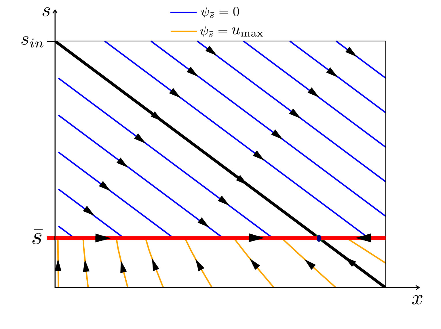 Figure 1
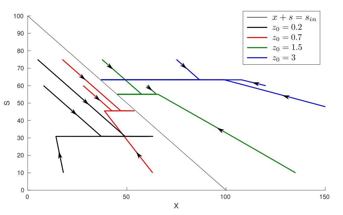 Figure 2
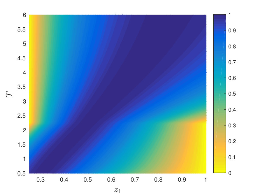 Figure 3
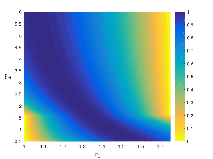 Figure 4
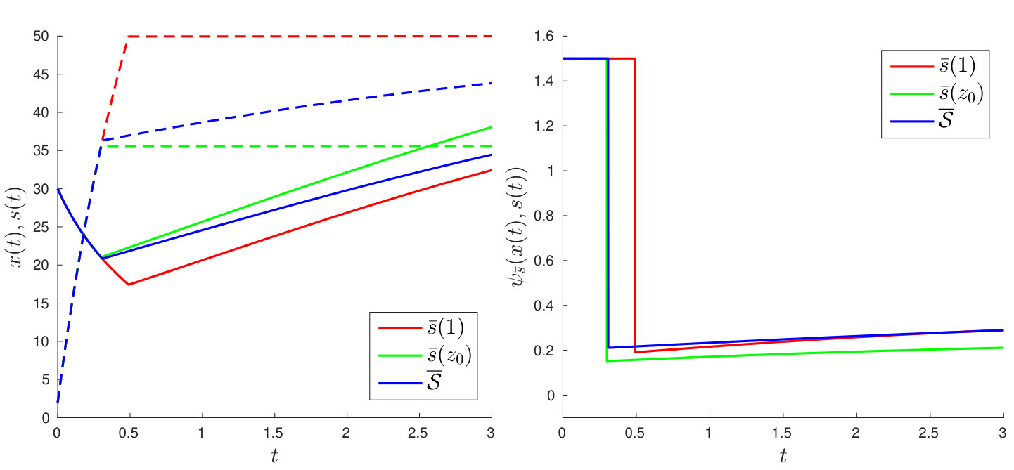 Figure 5
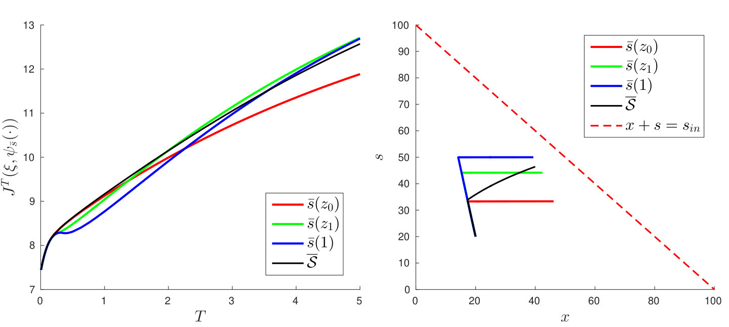 Figure 6
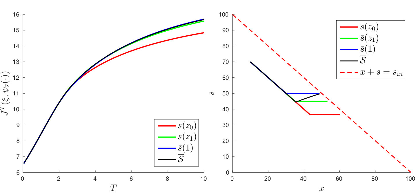 Figure 7
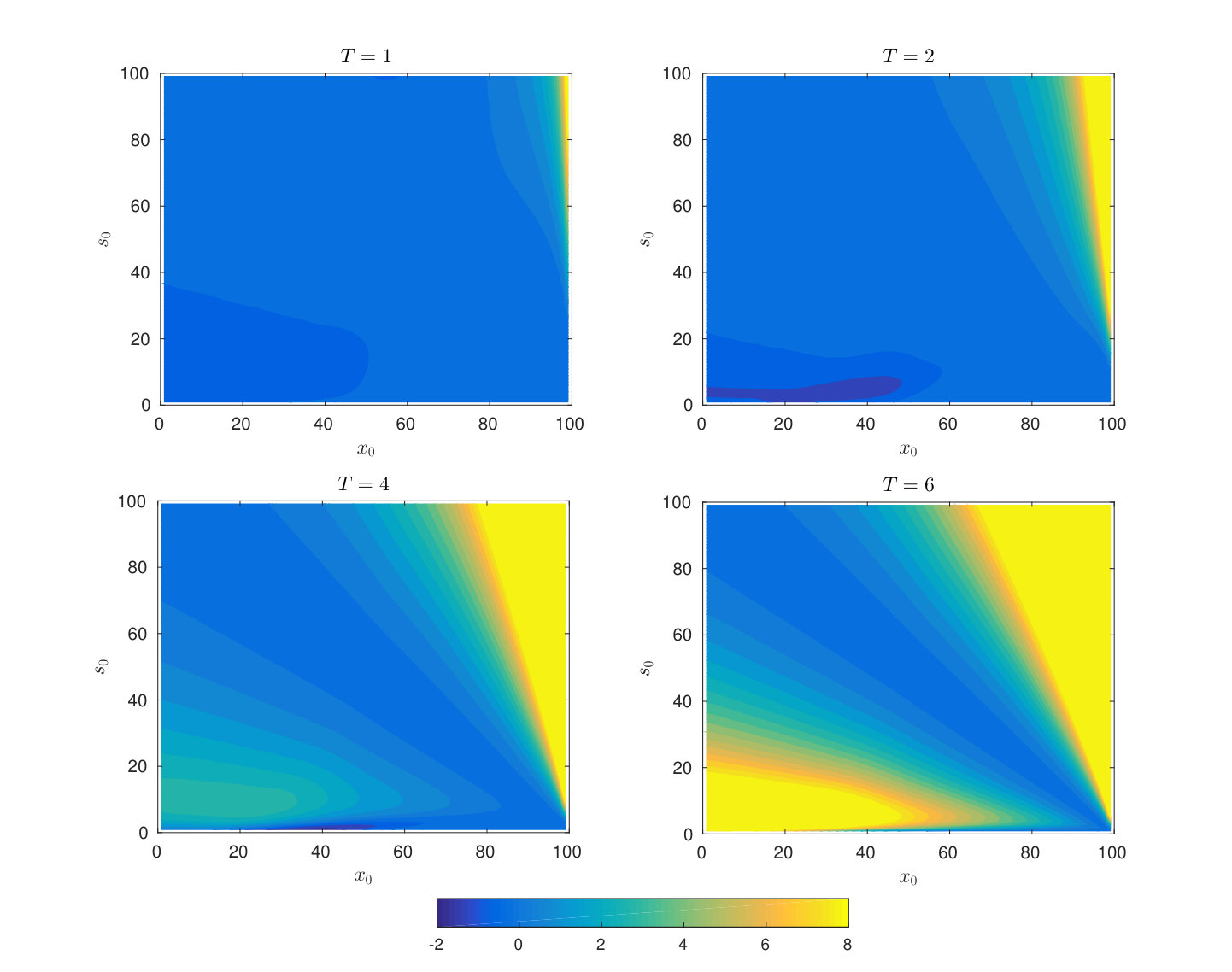 Figure 8
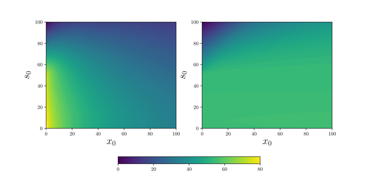 Figure 9
Peer Reviews
No public reviews on file for this paper yet. If you reviewed it on a platform where reviews are public (OpenReview, ICLR, NeurIPS, ICML), you can paste yours below so the community can read it here.
Videos
No videos yet. Explain this paper in a talk, walkthrough, or lecture? Add one.
Taxonomy
TopicsAdvanced Control Systems Optimization · Climate Change Policy and Economics · Anaerobic Digestion and Biogas Production
Optimal and Sub-optimal Feedback Controls
for Biogas Production
Antoine Haddon1,2
Héctor Ramírez1
Alain Rapaport2
(1 Mathematical Engineering Department and Center for Mathematical Modelling (CNRS UMI 2807), Universidad de Chile, Beauchef 851, Santiago, Chile ([email protected])
2 MISTEA, Université Montpellier, INRA, Montpellier SupAgro, 2 pl. Viala, 34060 Montpellier, France )
Abstract
We revisit the optimal control problem of maximizing biogas production in continuous bio-processes in two directions:
- over an infinite horizon,
- with sub-optimal controllers independent of the time horizon. For the first point, we identify a set of optimal controls for the problems with an averaged reward and with a discounted reward when the discount factor goes to 0 and we show that the value functions of both problems are equal. For the finite horizon problem, our approach relies on a framing of the value function by considering a different reward for which the optimal solution has an explicit optimal feedback that is time-independent. In particular, we show that this technique allows us to provide explicit bounds on the sub-optimality of the proposed controllers. The various strategies are finally illustrated on Haldane and Contois growth functions.
Keywords : Optimal control, Chemostat model, Singular arc, Sub-optimality, Infinite horizon.
1 Introduction
Anaerobic digestion is a biological process in which organic matter is transformed by microbial species into biogas (such as methane and carbon dioxide). Such transformations have been used for a long time in waste water-treatment plants to purify water [1]. Valorizing biogas production while treating wastewater has received recently great attention, as a way for producing valuable energy and limiting the carbon footprint of the process [2]. As a final product of the biological reaction, the total production of biogas measures the performances of the biological transformation. Therefore, there is a strong interest in determining control strategies maximizing biogas production.
With continuous-stirred bioreactors, two kinds of anaerobic models are usually considered for control purposes in the literature: the one-step model, which corresponds to the classical chemostat model [3], and the two-step model that has been proposed by Bernard et al. [4].
Although these models only have few dynamic variables, it has been shown that they are capable of reproducing the qualitative behavior of the anaerobic digestion process [5]. Furthermore, in the two-step model, the second reaction is the most limiting due to inhibition by the substrate and we can then consider that a one-step model can be used to focus on the second reaction. In particular, a common assumption is to consider that the first step is fast and then the two reactions can be reduced to a single one with a slow-fast approximation and in this case, the one-step model provides a good representation of the biogas production.
The control variable is typically the input flow rate (or equivalently the dilution rate, since the volume of the reactor is constant in continuous operating mode). Several works have already considered the static optimization problem of maximizing the output flow rate of biogas at steady state, and various control strategies have been proposed to stabilize the processes at these nominal states (see for instance [6, 7, 8, 9, 10, 11, 12]).
There has been comparatively much less work considering the dynamic optimization problem over the transients, while bio-processes are often not initialized at their optimal nominal state. Although the optimal control problem, which consists in maximizing biogas production over a given time interval, has been posed a long time ago [13], it is still unsolved today (even for the one-step model). Let us mention two attempts to solve approximately or partially this problem. Sbarciog et al. [14] have considered the two-step anaerobic model and proposed a strategy for maximizing biogas production as an optimal control to drive the system in finite time in a neighborhood of the optimal steady state, with additive penalty terms in the criterion. In [15], Ghouali et al. give a complete solution of the original optimal control problem for the one-step model, but for a particular subset of initial conditions which belong to an invariant manifold of the system (see also [16]). The dynamics can be then reduced to a scalar one and the authors show that the optimal solution exhibits a singular arc with a “most rapid approach path” optimal strategy. Let us underline that optimal control problems over a fixed time horizon possess generally a time-dependent optimal synthesis, while the duration of process operation is often poorly known. However, the scalar reduced problem exhibits the remarkable feature of having an optimal synthesis independent of the terminal time, which makes it quite attractive from an application view point.
The purpose of the present article is to propose new control strategies for the one-step model, as time-independent feedbacks for general initial conditions
either considering an infinite horizon,
- -
either considering sub-optimal controllers for the finite horizon.
For the infinite horizon (see for instance the book [17]), we consider the limit of the discounted criterion (when the discount factor tends to zero) and the average cost. We study optimal strategies and compare their related optimal costs. This study extends the preliminary results presented in the conference paper [18] and considers a large class of growth functions, that can be in particular density-dependent (such as the Contois law) or not (such as the Monod or Haldane law). Our work for the finite horizon exploits and extends an approximation technique presented in [19]. This consists, for a given initial condition, in framing the optimal solution by considering a different reward for which the optimal solution can be determined exactly and that possess the property of having a time-independent optimal synthesis (i.e. whatever is the time horizon, finite or infinite). This technique has moreover the advantage of providing bounds on the sub-optimality of the controllers. The results are again obtained for a large class of growth functions and we show that density dependent growth functions lead to more sophisticated feedback laws.
The paper is organized as follows. Section 2 specifies dynamics, control, criterion and hypotheses, and gives some preliminary results about controllability and asymptotic behavior of solutions. Sections 3 and 4 study the optimal solutions, respectively for the infinite and finite time horizons. Finally, Section 5 illustrates our results on various growth functions.
2 Preliminaries
In this work, we consider the classical chemostat model [3]. This represents a well-mixed continuously fed bioreactor in which a substrate of concentration is treated (and then transformed into biogas) by a population of microorganisms of concentration
[TABLE]
We denote the inflow concentration of substrate, the yield coefficient, the specific growth rate and the dilution rate, which is the control.
The biogas flowrate is assumed proportional to the growth rate so that the biogas produced during a time interval is proportional to
[TABLE]
and, without loss of generality, we will suppose that the proportionality coefficient as well as the yield coefficient are equal to 1.
We will consider the following class of growth functions :
Assumption 1**.**
We suppose that is a Lipschitz continuous function that satisfies, for all
[TABLE]
We suppose as well that is non increasing, which models crowding effects, and is non decreasing, which models the fact that having more biomass provides at least the same growth.
A typical instance of this class is the Contois growth function, defined later in (38), but note that this class of functions also contains growth functions that depend only on the substrate concentration, such as the Monod (36) and the Haldane (37) functions.
We will study the problem of maximizing the accumulated biogas for controls in the following set of admissible controls
[TABLE]
with and , and where is a given parameter that represents the maximal dilution rate. We will consider initial conditions taken in the invariant set
[TABLE]
which corresponds to the most common operating conditions. Notice that for initial conditions in , any solution of (1)-(2) cannot reach in finite time and stays non negative. Therefore the set is (forward) invariant.
2.1 Properties of the Dynamics
On the invariant domain , we introduce the change of variables
[TABLE]
under which the dynamics become
[TABLE]
We will denote and the solution of (7), with initial condition and control . The cumulated biogas production becomes
[TABLE]
with
[TABLE]
and we will denote
[TABLE]
We can now establish an important property of the controlled dynamics.
Lemma 1**.**
The trajectories of the system (7) for a given initial condition , for all admissible controls, remain in the set
[TABLE]
Proof.
From Assumption 1 we have that and since the solutions satisfy (7), we then have the following
[TABLE]
for all , for any admissible control . ∎
In the following, we consider initial conditions that guarantee the controllability of the variable.
Assumption 2**.**
We suppose that the initial condition is such that
[TABLE]
In practice, for a given initial condition it possible to choose such that the previous inequality is satisfied.
We now define a class of feedbacks, that will play an important role, and that are based on the notion of most rapid approach path, a well known concept in the theory of optimal control, see for example [20, 21].
Definition 1**.**
For , we define the most rapid approach feedback to a given substrate level , as
[TABLE]
Clearly, with Assumption 2 this feedback is well defined, so that, associated with this control, for every initial condition , there exists a unique absolutely continuous solution for the dynamics (7).
Lemma 2**.**
For any satisfying Assumption 2, a given substrate level is reachable in finite time with the feedback .
Proof.
First, using the monotonicity properties of of Assumption 1, it is clear that is admissible provided Assumption 2 is satisfied.
To show that is reachable in finite time, it is enough to note that when , for in a given open interval , we have
[TABLE]
with k_{-}=-\min_{s\in(s^{*},s_{in})}\mu\big{(}s,(s_{in}-s)\min(z_{0},1)\big{)}\min(z_{0},1)(s_{in}-s^{*}). This insures that is always reachable in finite time from .
Analogously, if , for , we have from Assumption 2
[TABLE]
with k_{+}=\left[u_{\max}-\max_{s\in(0,s^{*})}\mu\big{(}s,(s_{in}-s)\max(z_{0},1)\big{)}\max(z_{0},1)\right](s_{in}-s^{*}). Then is reachable from , again in finite time.
∎
Remark 1**.**
It should be pointed out that there is a similarity with the turnpike property [22, 23] when using the controller (12). The turnpike property has received great attention in the literature (see for instance [24, 20, 21, 25]), and recent results give sufficient optimality conditions [26, 27]. However, we shall show in the next sections that the value , which determines the turnpike, has to depend on the initial condition (excepted for the very particular case when the initial condition belongs to the invariant set that has been solved in [15]). So, we are not in the usual framework of a single turnpike [26, 27] or isolated turnpikes [28], and the results of the literature do not apply.
For the problem on an infinite horizon, we will consider persistently exciting controls, which are defined as satisfying
[TABLE]
As the next Lemma shows, the trajectories associated with these controls are such that converges to 1, which is essential in our approach. Furthermore, for non persistently exciting controls, converges to 0 and thus the biogas production also converges to 0. As a consequence, the controls that maximize biogas production are necessarily persistently exciting controls.
Lemma 3**.**
For all initial conditions and for all persistently exciting controls , we have
[TABLE]
and
[TABLE]
Moreover, for non persistently exciting controls, we have
[TABLE]
Proof.
From equation (7), the solution can be written as follows
[TABLE]
where , . From equation (2), the solution is such that
[TABLE]
Therefore, if the integral function
[TABLE]
is bounded, then must converge asymptotically to [math] when goes to and is a persistently exciting control. Moreover, from equations (1), (2) we have
[TABLE]
so that
[TABLE]
and then must converge to when goes to . Consequently, by continuity of the function , there exists such that
[TABLE]
for any , which implies that the integral defined in (14) goes to when goes to , which is a contradiction. We deduce that this integral cannot be bounded and from equation (13) that converges to when goes to .
A proof of the equality of limits of the integrals
[TABLE]
can be found in [29, Lemma 3.5]. For the value of the limits we use the fact that converges to 1 : for all , there exits a time such that, for all ,
[TABLE]
Then, for all
[TABLE]
With this, for all , we can take and then we have, for
[TABLE]
Finally, we prove that for non persistently exciting controls, converges to 0. Therefore, suppose that is an admissible control with a finite integral and we define, for all ,
[TABLE]
and
[TABLE]
Then
[TABLE]
and since is bounded, we can deduce that converges as goes to infinity. Note as well that is absolutely continuous and thus uniformly continuous. We can therefore use Barbalat’s Lemma [30, Lemma 4.2] to get that converges to 0. Then, as cannot reach 0 (Lemma 1), we have that \phi\big{(}s_{0,\xi,u}(t),z_{0,\xi,u}(t)\big{)} must converge to 0 and by continuity we conclude that converges to 0.
∎
3 Infinite Horizon and Average Reward
In this section, we study the problem of maximizing biogas production over an infinite horizon. Since the dynamics (7) are autonomous, without loss of generality, we can assume here that and we will then denote and solutions of (7).
We start by defining the average biogas production during a time interval as
[TABLE]
and we consider the inferior and superior limits as goes to infinity
[TABLE]
The optimal control problems in consideration here consist in maximizing these functionals with respect to the dilution rate , for any initial condition . More precisely, the value functions of these optimal control problems are
[TABLE]
We need to consider the inferior and superior limits here as there exists controls for which the rewards (16) and (17) may differ. Indeed, this is the case for certain oscillating controls as can be seen in the example in the Appendix. Nevertheless, we will show that the value functions (18) and (19) are in fact equal. Moreover, we will connect these problems to the problem with a discounted reward when the discount factor goes to 0, as in [31], and we will identify a set of controls that are optimal for all three problems.
To this end, we now define the following discounted reward, for a discount rate
[TABLE]
This type of cost function is often used in problems related to economics for which the term represents a discount rate or a preference for the present [17]. In our setting, the use of this discounted reward can be seen as a preference for earlier rather than later production. Here, the integral is rescaled with the discount factor in order to guarantee that, when we take the limit as goes to 0, the reward remains finite.
The value function of the optimal control problem for a given is then
[TABLE]
Note that both average rewards (16) and (17), as well as the discounted reward (20), are well defined as the following Lemma shows.
Lemma 4**.**
For all , for all admissible controls and for all , the rewards , and are uniformly bounded.
Proof.
From the monotonicity properties of Assumption 1, we have that the function is non increasing. for all . Thus, for all
[TABLE]
The uniform boundedness of the rewards then follows from Lemma 1.
∎
3.1 Relation Between Average and Discounted Biogas Production Problems
We now show how the average and discounted biogas production problems are related when the discount factor goes to 0.
In the following, we will consider the discounted reward (20) as a function of the trajectory \zeta(\cdot)=\big{(}s_{\xi,u}(\cdot),z_{\xi,u}(\cdot)\big{)} instead of the control and with a slight abuse of notation, we will denote it as . Define the set valued map
[TABLE]
and consider the set of all forward trajectories of (7) with initial condition
[TABLE]
where denotes the set of absolutely continuous functions from to . We recall from the Filippov Selection Theorem (see for instance [32]) that the optimal control problem (21) is equivalent to the optimization problem on ,
[TABLE]
We now specify the topology that we will use to study the limit of the discounted biogas production problem when the discount factor goes to 0.
Definition 2**.**
For , we denote by L^{1}\big{(}0,\infty;\mathbb{R}^{2},e^{-bt}dt\big{)} the weighted Lebesgue space of measurable functions from to such that
[TABLE]
and we denote W^{1,1}\big{(}0,\infty;\mathbb{R}^{2},e^{-bt}dt\big{)} the weighted Sobolev space of measurable functions satisfying
[TABLE]
We consider the topology on W^{1,1}\big{(}0,\infty;\mathbb{R}^{2},e^{-bt}dt\big{)} for which a sequence converges to if and only if
* converges uniformly to on compact intervals,*
- -
* converges weakly to in L^{1}\big{(}0,\infty;\mathbb{R}^{2},e^{-bt}dt\big{)}.*
Now, we define the notion of limit in our context (see [33] for further details).
Definition 3**.**
For a given initial condition and trajectory , the lower limit and upper limit of are
[TABLE]
Here, we denote the set of all open neighborhoods of of the topology on W^{1,1}\big{(}0,\infty;\mathbb{R}^{2},e^{-bt}dt\big{)} given in Definition 2. If both of these limits coincide, then the limit of is
[TABLE]
We now show that this limit is well defined, as well as the associated optimal control problem.
Proposition 1**.**
For all and for all trajectories , the limit of exists and we denote it as
[TABLE]
In addition, for all , the suprema are attained
[TABLE]
and these maxima converge as goes to 0, pointwise in ,
[TABLE]
Finally, if is an optimal trajectory for (21), i.e. if , and if converges to in , then is an optimal control for (22) and
[TABLE]
Proof.
First, we show that for all trajectories \zeta(\cdot)=\big{(}s(t),z(t)\big{)}\in{\cal S}(\xi) and for small enough, is increasing. We can write this function as
[TABLE]
with g(t):=\phi\big{(}s(t),z(t)\big{)}z(t), which is bounded and positive (Lemma 1),
[TABLE]
Then, we have
[TABLE]
so that for ,
[TABLE]
Now, since , there exists such that, for all , \frac{m}{\delta}\big{(}1-e^{-\delta T})>\frac{mT}{2}. Then, taking , we conclude that is increasing for .
Next, recall that for all initial conditions and all trajectories, is uniformly bounded (Lemma 4). Finally, since is continuous with respect to , we can use [33, Proposition 5.7] to get the convergence as goes to 0.
To show that the suprema are attained and that they converge, it is sufficient to show that there exists a countably compact set on which the suprema are attained for all [33, Theorem 7.4]. The set is clearly independent of so that we now need to show that is countably compact for the topology on W^{1,1}\big{(}0,\infty;\mathbb{R}^{2},e^{-bt}dt\big{)} given in Definition 2. However, since W^{1,1}\big{(}0,\infty;\mathbb{R}^{2},e^{-bt}dt\big{)} is a metric space, any compact set is countably compact, so we only need to prove the compactness of .
For each we set
[TABLE]
where is the projection on the convex set . Then has linear growth, so that we can define
[TABLE]
where . Note that is upper semi-continuous and has compact non-empty convex images (such a map is known as a Marchaud map [34]). With this, the set is the set of absolutely continuous solutions of the differential inclusion
[TABLE]
We can therefore use [34, Theorem 3.5.2] to establish that is compact in W^{1,1}\big{(}0,\infty;\mathbb{R}^{2},e^{-bt}dt\big{)} for .
∎
We now relate the average and discounted biogas production problems.
Proposition 2**.**
For all we have
[TABLE]
Proof.
We adapt here results of [31] given for minimization problems to maximization problems by changing the sign of the reward. We give here the main steps for the first inequality, the second is obtained similarly. First, [31, Lemma 3.3] gives
[TABLE]
and then [31, Corollary 3.5] states that for all , all we have
[TABLE]
for all small . Taking the limit as and gives the result.
∎
3.2 Solution of Optimal Control Problems
We now solve the optimal control problems (18) and (19) and show that their value functions are equal to the limit (22) of the discounted problem. We start by determining an upper bound for the value functions and then we will exhibit controls that attain this bound.
Proposition 3**.**
For all initial conditions
[TABLE]
Proof.
With the monotonicity properties of of Assumption 1, we have that is non increasing and is non decreasing. This implies that
[TABLE]
and
[TABLE]
First, we consider the case when . For any control , we have
[TABLE]
Taking the upper limit as goes to infinity and the supremum with respect to we get the result.
Next, for , we have
[TABLE]
Using Lemma 3 we get that and we conclude taking the supremum with respect to .
∎
Note that the existence of a maximum of on follows from Assumption 1. We will denote a substrate level at which such a maximum is attained as
[TABLE]
Proposition 4**.**
For any initial condition , any control that drives the system asymptotically to the state is optimal for problems (18), (19) and (22). We then have
[TABLE]
Proof.
The continuity of implies that for all , there exists a time such that, for all ,
[TABLE]
Since and take values in the compact set (11), there is a constant such that, for all ,
[TABLE]
Then, for all , from (26) and (27)
[TABLE]
and we have
[TABLE]
Using Propositions 2 and 3, we get the equality of value functions (25) and deduce the optimality of for both average biogas production problems (18) and (19). We proceed similarly to get
[TABLE]
and we have
[TABLE]
Then, Proposition 2 implies that is also optimal for problem (22).
∎
With Lemma 3, we know that all persistently exciting admissible controls make converge to 1, and from Lemma 2, we know that the feedback defined in (12) with guarantees that reaches . Then, from the previous Proposition we have the following result.
Proposition 5**.**
For any initial condition satisfying Assumption 2, the most rapid approach feedback to , defined in (12) and denoted , is optimal for both average production problems (18) and (19) and for the limit (22) of the discounted production problem.
Clearly, there is not a unique optimal control for the infinite horizon problems that we have considered. For example, in the case of a growth function that depends only on the substrate and that is monotone (such as the Monod growth function), the constant control can also drive the system to the state . Nonetheless, for the control , we are able to state in the next section an estimation of the sub-optimality for the finite horizon problem.
4 Finite Horizon and Sub-optimal Controls
We now examine the problem of maximizing biogas production over a finite horizon for a time interval where is fixed. For this we consider the following reward
[TABLE]
where we recall that \big{(}s_{t_{0},\xi,u}(\cdot),z_{t_{0},\xi,u}(\cdot)\big{)} is the solution of (7) with control and initial condition . The optimal control problem consists in maximizing this functional with respect to the dilution rate, so that the associated value function is
[TABLE]
We also consider auxiliary optimal control problems, which consist in maximizing the cost, for a given ,
[TABLE]
for the same dynamics (7). The value functions of these auxiliary problems are then defined as
[TABLE]
The resolution of these auxiliary problems will be presented in Section 4.1.
We now show that the value functions of the original problem (29) and the auxiliary problems (31) are related.
Proposition 6**.**
For all , and any , we have the following frame for the value function of the original problem
[TABLE]
Proof.
We start with the case . For a given control , we define the following time
[TABLE]
which it is well defined since is monotonous. Then, for we have and with the monotonicity properties of of Assumption 1 we have
[TABLE]
Next, for we have and
[TABLE]
Combining these inequalities we get
[TABLE]
Now, since we have
[TABLE]
For the case , we proceed in a similar way to get
[TABLE]
We conclude by taking the supremum over all admissible controls.
∎
The interest of the previous frames on the value functions is that it allows to find controls for which we have an estimation of sub-optimality for the original problem.
Proposition 7**.**
For all and all , any optimal control for the reward guarantees a (sub-optimal) value for the original criterion that satisfies
[TABLE]
and we have the following estimation of the value function
[TABLE]
Proof.
From the proof of Proposition 6, for any control , we have
[TABLE]
Evaluating this for any optimal control for the reward gives the sub-optimality frame (33). The sub-optimality estimation (34) then follows from (32) and (33).
∎
4.1 Resolution of Auxiliary Problems
In order to obtain sub-optimal controls for problem (29) we now need to solve the auxiliary problem (31) for a given . The optimal control of this auxiliary problem is an autonomous feedback, even though the horizon is fixed and finite. It is similar to the optimal feedback for the infinite horizon problem , defined in (12), and it drives the system towards a maximizer of but now, this maximizing substrate level depends on .
We first need an assumption on the uniqueness of a maximum of .
Assumption 3**.**
For each , the function admits a unique maximum on , and we denote the substrate level at which this maximum is attained as
[TABLE]
Note that implies that is increasing on and decreasing on .
Proposition 8**.**
For all satisfying Assumption 2 and all , the most rapid approach feedback to , defined in (12) and denoted , is optimal for the auxiliary problem (31).
Proof.
We start with the case . With the control , the solution of (7) is such that is monotonic and non increasing. Therefore there exists a time , possibly larger than , such that and then the solution with the feedback (12) is, with
[TABLE]
Next, for all and for all ,
[TABLE]
By the theorem of comparison of solutions of scalar differential equations, this implies that , up to time , for all controls . Since is decreasing on , we have
[TABLE]
Finally, as reaches its maximum at we get
[TABLE]
We now consider . From Assumption 2, the feedback is admissible and we have
[TABLE]
Thus, with the control , the solution of (7) is such that is monotone and non decreasing. Therefore, there exists a time , possibly larger than , such that and then the solution with the feedback (12) is, with
[TABLE]
Next, for all and for all
[TABLE]
and this implies that , up to time , for all controls . Since is increasing on , we have
[TABLE]
Finally, since reaches its maximum at , we get
[TABLE]
∎
5 Application to Particular Growth Functions
The controls that we have considered up to now are all most rapid approach feedbacks to , with , and this leads to the question of which is best in terms of biogas production. It turns out that it depends on the initial conditions and the horizon considered.
Indeed, we know that for an infinite horizon, the feedback with is optimal and we can then expect that when the horizon is large, the best of the considered feedbacks would be for close to 1. On the other hand, when the horizon is small, the feedback would seem to be the best option since this strategy consists in remaining close to the maximum of the biogas flow rate corresponding to the initial condition, whereas another feedback could drive the system away, towards another maximizing state but that can not be reached in time.
In this section, we apply our main results to the most common growth functions and explore with numerical simulations the question of determining the best feedback for a given initial condition and final time. In particular, we will work with the Monod function
[TABLE]
the Haldane function
[TABLE]
and the Contois function
[TABLE]
where , , and are positive numbers. We shall see later that these functions satisfy our assumptions (Lemma 5).
First, note that the Monod and Haldane functions only depend on the substrate, so that in this case, the maximizers , defined in (35), are all equal to , for all . We illustrate the associated feedback for a Haldane function with a graph of the state space trajectories in Figure 1. The case of a Monod function leads to a similar dynamical behavior and the only major difference is the value of .
From now on we will only consider the Contois growth function, for which we plot the trajectories in state space obtained with the feedback in Figure 2.
To determine which of the feedbacks is the best, we now compute the associated reward for a range of values of and of final times for a given initial condition. In order to easily identify the maximum of with respect to , we normalize the average reward (15) by computing
[TABLE]
where the minimum and maximum are taken for . Hence, for each final time , the maximum reward is achieved for such that and the minimum when .
Figure 3 shows a case when and Figure 4 is an example of . We can see clearly that for small final times, the maximum is attained for a value of close to and that for the reward is the smallest. However, as the final time increases, the value of for which the reward is maximum approaches 1, and with the feedback the reward is the smallest. In particular, we can see that the best of the feedbacks depends on the final time.
This leads us to consider a new feedback that keeps the system in the set of maximizers
[TABLE]
We therefore introduce the following most rapid approach feedback to
[TABLE]
where is the feedback that keeps the system in the set , that we compute by differentiating with respect to time the equation .
We first illustrate this feedback in Figure 5 where we show the states as functions of time and the open loop realizations of the feedbacks , and . Next, in Figure 6 we compare the reward of the feedback to the others and we can notice that the reward associated with the feedback is always one of the best, although for any given final time it is possible to do better with a feedback for the right .
Note also that the feedback will drive the system asymptotically towards the state so that it is also optimal for the infinite horizon problems (18), (19) and (22).
In Figure 8, we show the difference between the rewards of the feedbacks and as a function of the initial condition for various final times.
From this, we see that the feedback that is best changes, depending on the initial condition and the horizon considered.
The sub-optimality estimation (33) is affected similarly, as this bound depends on the initial condition and in particular, the distance to the set has a major impact on the sub-optimality of the considered feedbacks. In addition, the growth function has an influence on our estimation, through , and we illustrate this in Figure 9 by plotting this value function for the Haldane and the Contois growth function. Observe that, for the Contois growth function, varies significantly with the initial biomass and thus the sub-optimality bound as well. This can be attributed to the dependence of the Contois growth function on biomass concentration and this effect is not seen with the Haldane growth function, which depends only on the substrate.
We finish this section with a Lemma that shows that the considered growth functions satisfy our assumptions.
Lemma 5**.**
For all positive , , and the Monod, Haldane and Contois growth functions satisfy Assumptions 1 and 3.
Proof.
Notice that the function with the Monod or Haldane function does not depend on . Let us show that the function is increasing and strictly concave
[TABLE]
Now, since the function is non-negative on and vanishes at 0 and it admits a maximum on . One has
[TABLE]
The function is thus strictly concave on , which provides the uniqueness of its maximum.
For the Haldane function, we have
[TABLE]
such that and and since is continuous it must have an odd number of zeroes in the interval . But notice that the equation admits at most 2 solutions and and therefore has a unique maximum.
For the Contois function, notice that so that, for
[TABLE]
and since is an increasing function, is also strictly concave.
∎
6 Conclusions
In this work, we have proposed a novel approach to obtain autonomous sub-optimal feedbacks for the open problem of maximizing biogas production in the chemostat model out of equilibrium. These controllers generalize the “most-rapid approach path” feedback control that is known to be optimal when the initial condition belongs to a certain manifold. Indeed, we obtain a family of feedback controls of similar structure, for which we are able to give bounds on the sub-optimality. This last point merits to be underlined as it usually difficult to evaluate a priori the performances of sub-optimality without having to determine or compute the optimal solution. This choice gives also flexibility for the practitioners to choose a controller depending on the time horizon or simply to pick one when the finite horizon is poorly known (as each controller guarantees a sub-optimality bound), or to adjust it when the horizon is changed. For infinite horizon we show that each controller guarantees the same optimal averaged cost.
This methodology, based on a framing of the dynamics, could be investigated for a larger class of dynamics, such as the two-step model, and be the matter of future work.
Acknowledgments
The first and second authors were supported by FONDECYT grant 1160567, and by Basal Program CMM-AFB 170001 from CONICYT-Chile. The first author was supported by a doctoral fellowship CONICYT-PFCHA/Doctorado Nacional/2017-21170249. The third author was supported by the LabEx NUMEV incorporated into the I-Site MUSE.
Appendix: A Particular Example
We construct here a control for which the average rewards (16) and (17) do not coincide. For this, let us consider an initial condition , with fixed. The set is clearly invariant for the dynamics (7) and therefore the chosen initial condition ensures that trajectories remains in this set.
Now consider the 2 following paths :
- (A)
Starting at , use the control to reach a prescribed level of substrate in finite time. Then, apply the control to return to in finite time, which is possible by Assumption 2. Denote this control by , and let be the (finite) time necessary to follow this path and be the biogas produced by this path. 2. (B)
Starting at , use to stay at for any time interval.
Then, define control as follows:
- •
For , set so that the biogas production for this period is .
- •
For , with , set in order to follow the path (A) repeatedly times. For each of these intervals the biogas production is .
- •
For , with , set . For each of these intervals the biogas production is .
Thus, when we apply control up to a time , for a given , the average biogas production is computed as follows
[TABLE]
which yields
[TABLE]
We have used here the fact that the sum converges to . Indeed, this follows from the identity
[TABLE]
However, for the same control , the average biogas production is, up to time , computed as follows
[TABLE]
which yields
[TABLE]
Since , it follows that , and consequently, . We thus obtain that
[TABLE]
The reference list from the paper itself. Each links out to its DOI / PubMed record.
- 1[1] Russell, D.: Practical wastewater treatment. Wiley (2006)
- 2[2] Rehl, T., Muller, J.: CO 2 abatement costs of greenhouse gas (GHG) mitigation by different biogas conversion pathways. Journal of Environmental Management 114 (15), 13–25 (2013)
- 3[3] Harmand, J., Lobry, C., Rapaport, A., Sari, T.: The Chemostat: Mathematical Theory of Microorganisms Cultures. Wiley, Chemical Engineering Series, Chemostat and Bioprocesses Set 1 (2017)
- 4[4] Bernard, O., Hadj-Sadok, Z., Dochain, D., Genovesi, A., , Steyer, J.P.: Dynamical model development and parameter identification for an anaerobic wastewater treatment process. Biotechnology and Bioengineering 75 , 424–438 (2001)
- 5[5] Bernard, O., Chachuat, B., Hélias, A., Rodriguez, J.: Can we assess the model complexity for a bioprocess: theory and example of the anaerobic digestion process. Water science and technology 52 (1), 85–92 (2006)
- 6[6] Steyer, J.P., Buffière, P., Rolland, D., Moletta, R.: Advanced control of anaerobic digestion processes through disturbances modeling. Water Research 33 (9), 2059–2068 (1999)
- 7[7] Rodríguez, J., Ruiz, G., Molina, F., Roca, E., Lema, J.: A hydrogen-based variable-gain controller for anaerobic digestion processes. Water Science and Technology 54 (2), 57–62 (2006)
- 8[8] Dimitrova, N., Krastanov, M.: Nonlinear stabilizing control of an uncertain bioprocess. Int. J. Appl. Math. Comput. Sci 19 (3), 441–454 (2009)