A Finite Volume Scheme for Savage-Hutter Equations on Unstructured Grids
Ruo Li, Xiaohua Zhang

TL;DR
This paper introduces a finite volume numerical scheme on unstructured grids for Savage-Hutter equations, effectively handling discontinuities and non-Galilean invariance, demonstrated through granular avalanche flow simulations.
Contribution
A novel Godunov-type finite volume scheme with a modified HLL flux for Savage-Hutter equations on unstructured grids, addressing non-Galilean invariance and discontinuities.
Findings
Scheme accurately captures shock waves in granular flows
Numerical results agree well with reference solutions
Applicable to complex avalanche simulations
Abstract
A Godunov-type finite volume scheme on unstructured triangular grids is proposed to numerically solve the Savage-Hutter equations in curvilinear coordinate. We show the direct observation that the model is a not Galilean invariant system. At the cell boundary, the modified Harten-Lax-van Leer (HLL) approximate Riemann solver is adopted to calculate the numerical flux. The modified HLL flux is not troubled by the lack of Galilean invariance of the model and it is helpful to handle discontinuities at free interface. Rigidly the system is not always a hyperbolic system due to the dependence of flux on the velocity gradient. Even though, our numerical results still show quite good agreements to reference solutions. The simulations for granular avalanche flows with shock waves indicate that the scheme is applicable.
Click any figure to enlarge with its caption.
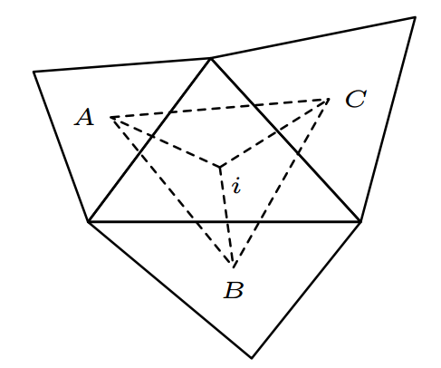 Figure 1
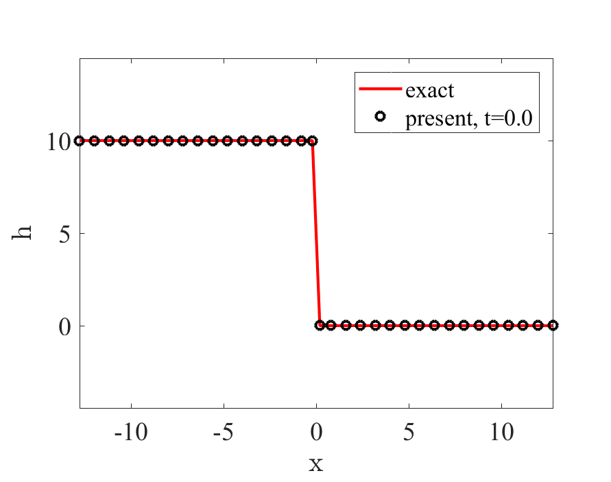 Figure 2
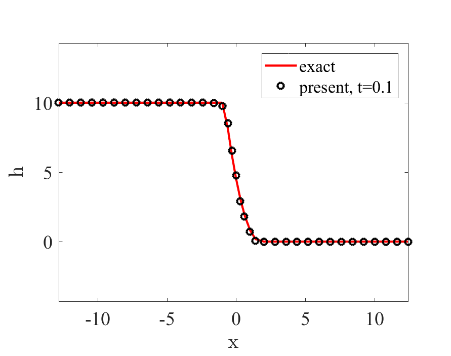 Figure 3
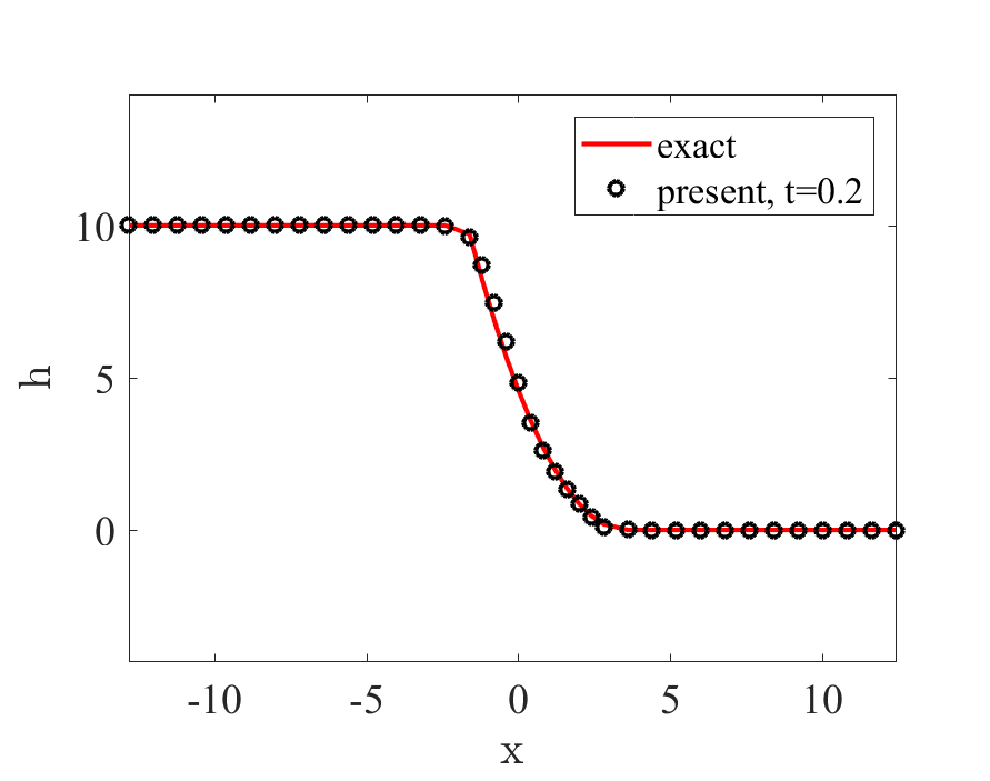 Figure 4
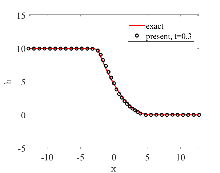 Figure 5
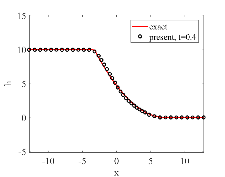 Figure 6
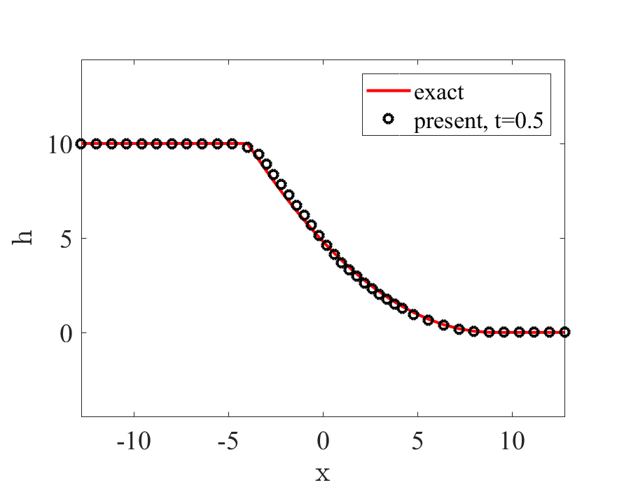 Figure 7
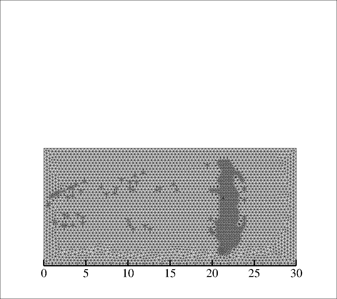 Figure 8
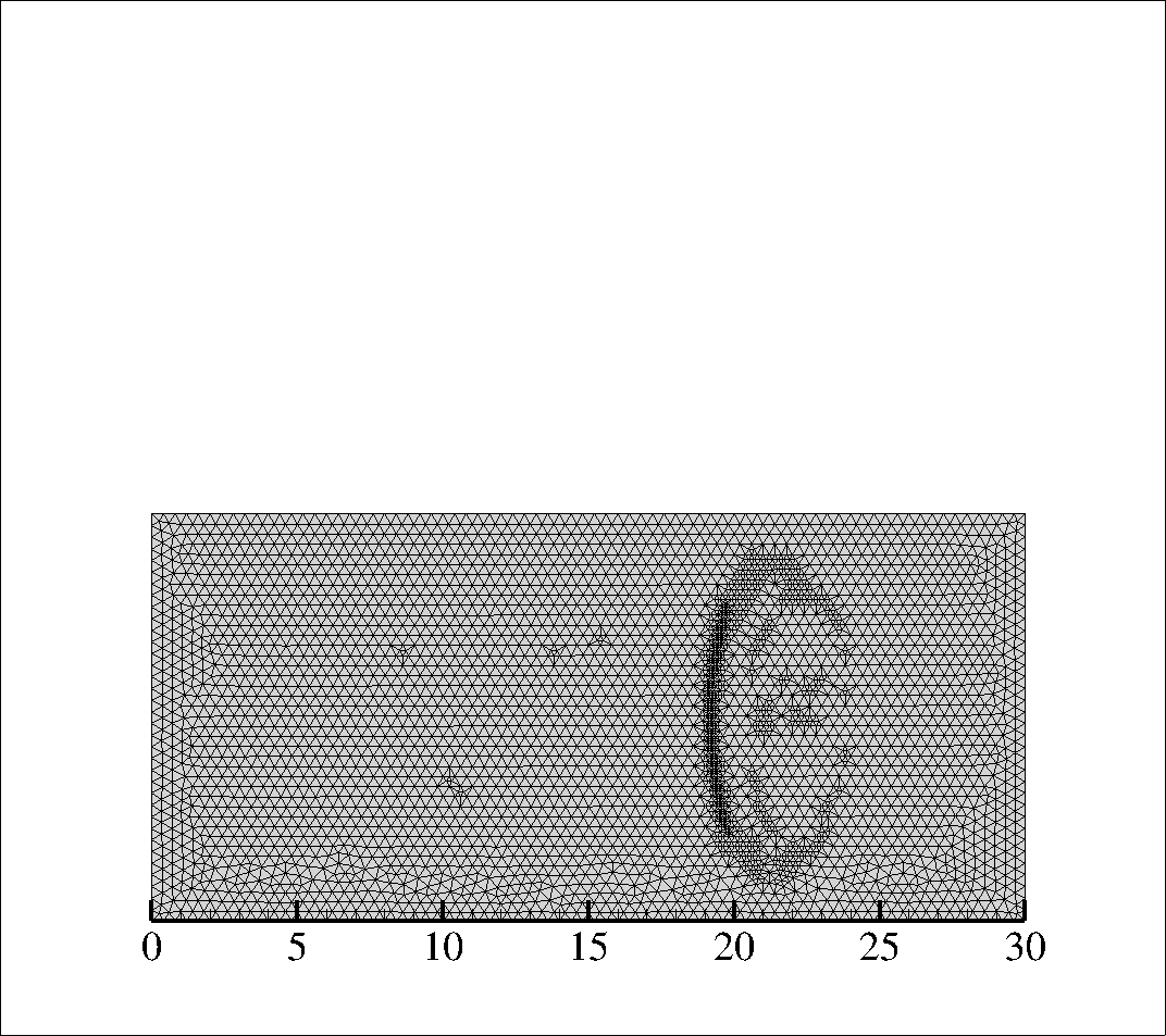 Figure 9
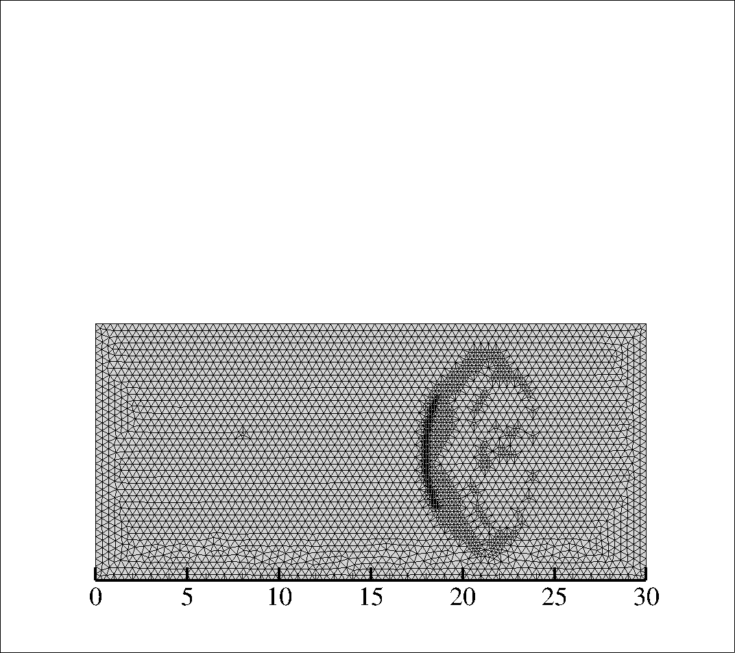 Figure 10
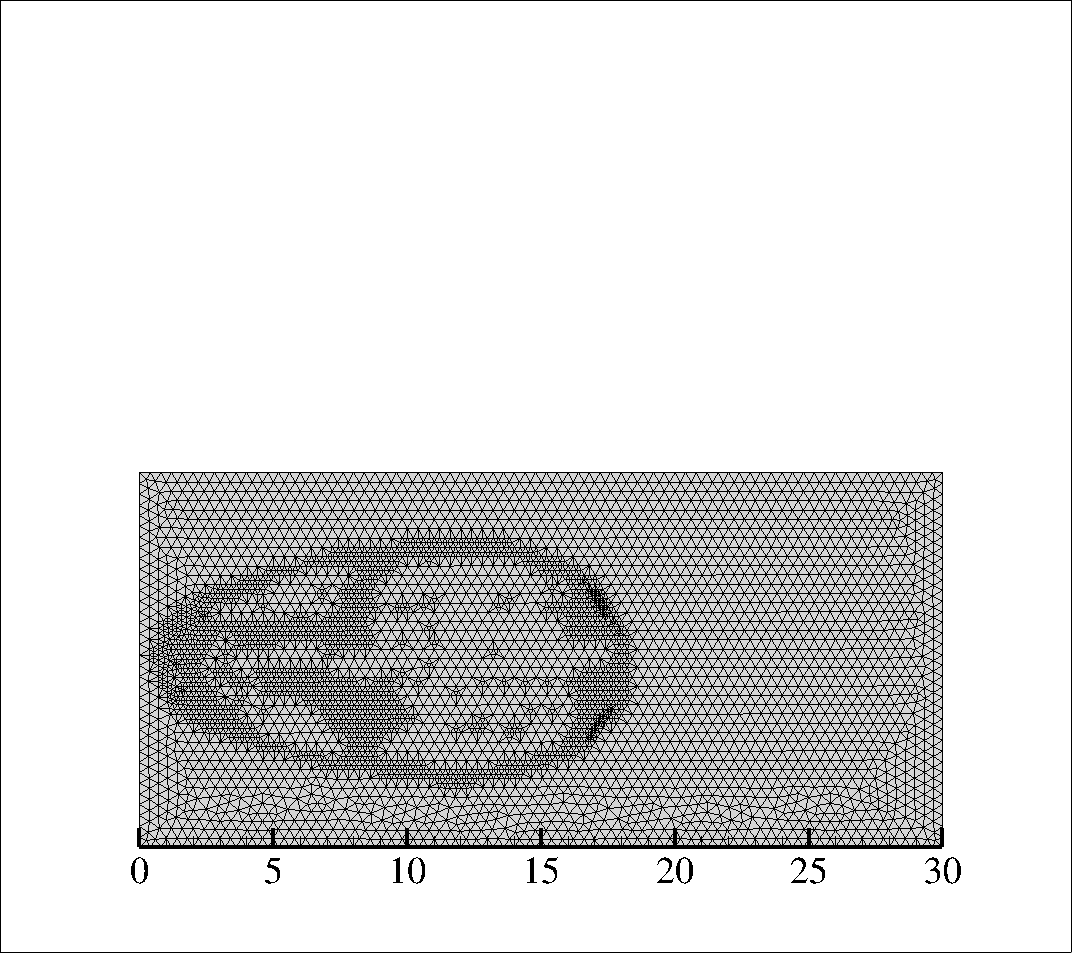 Figure 11
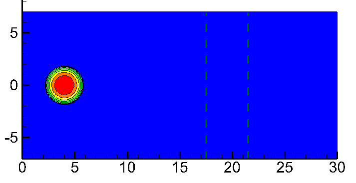 Figure 12
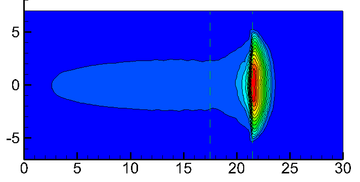 Figure 13
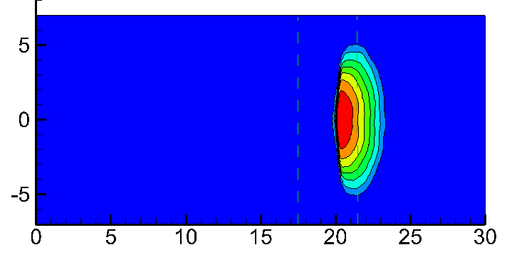 Figure 14
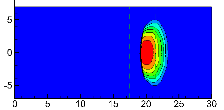 Figure 15
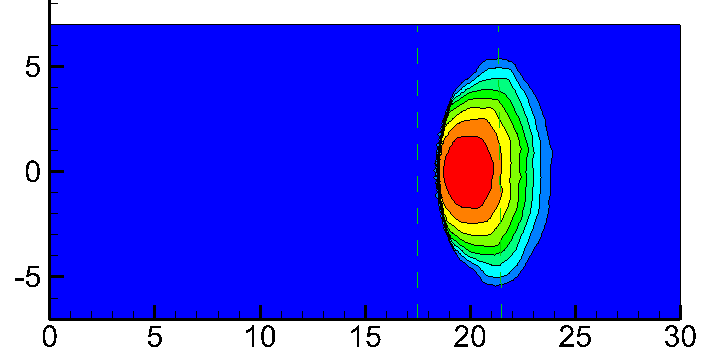 Figure 16
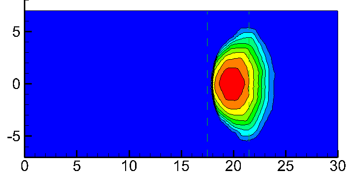 Figure 17
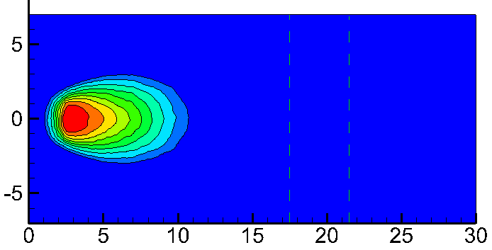 Figure 18
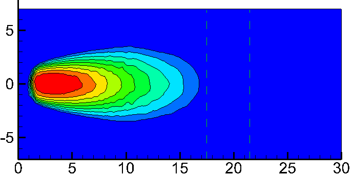 Figure 19
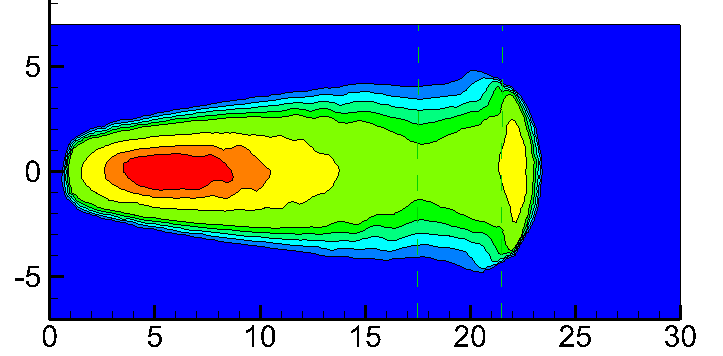 Figure 20
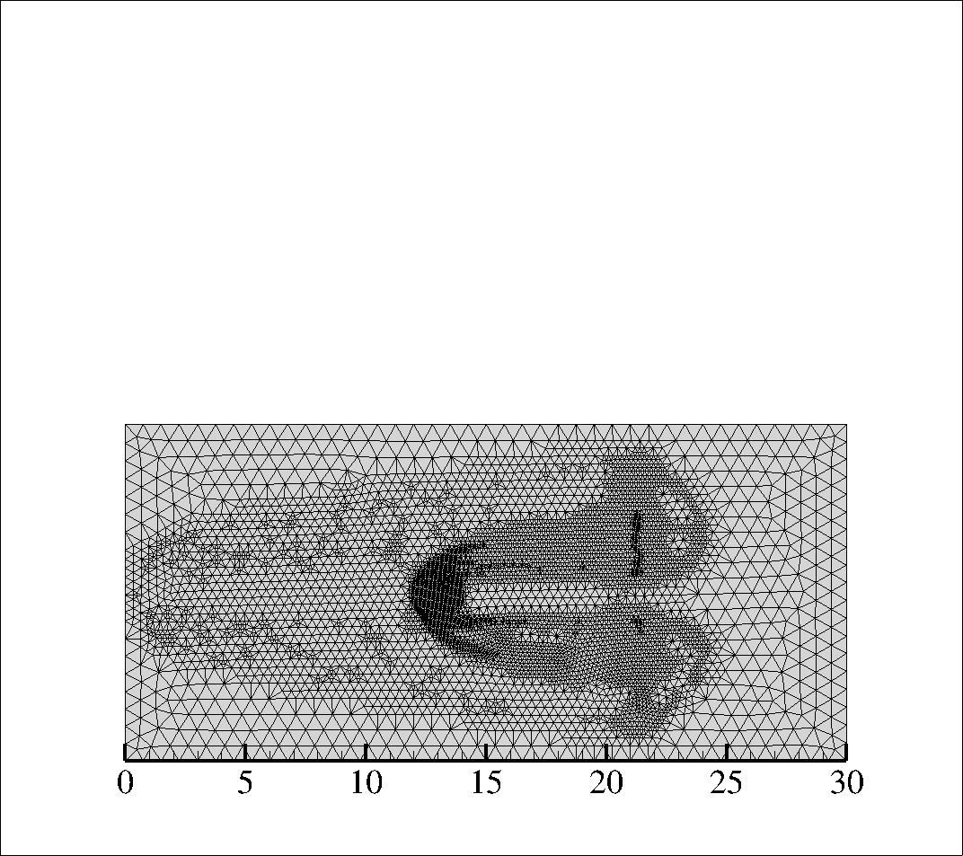 Figure 21
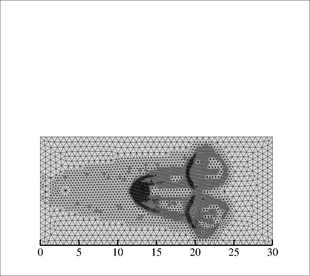 Figure 22
 Figure 23
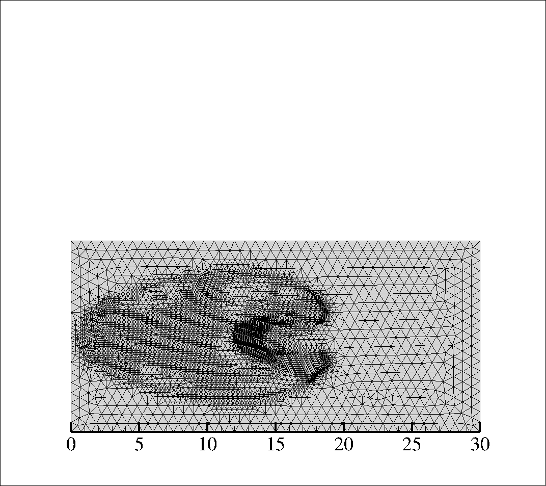 Figure 24
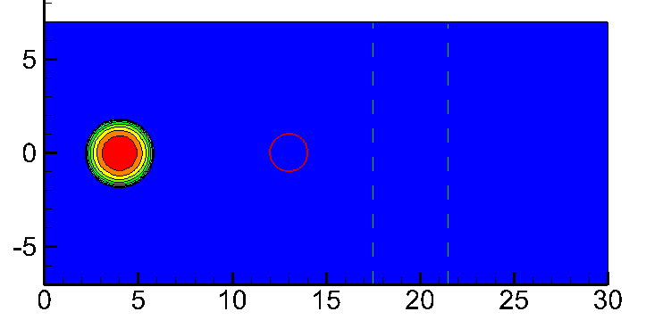 Figure 25
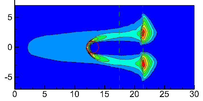 Figure 26
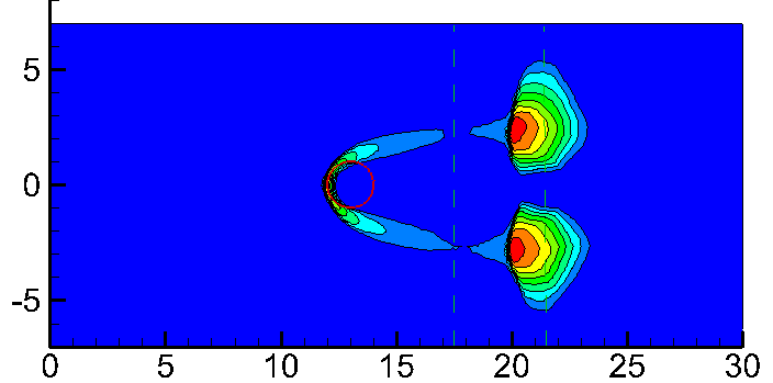 Figure 27
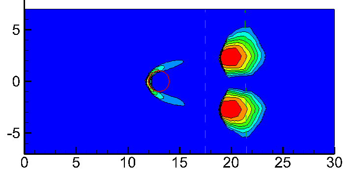 Figure 28
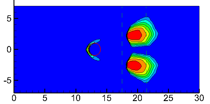 Figure 29
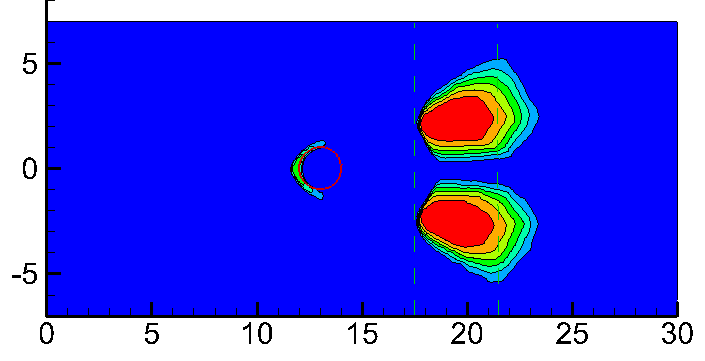 Figure 30
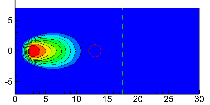 Figure 31
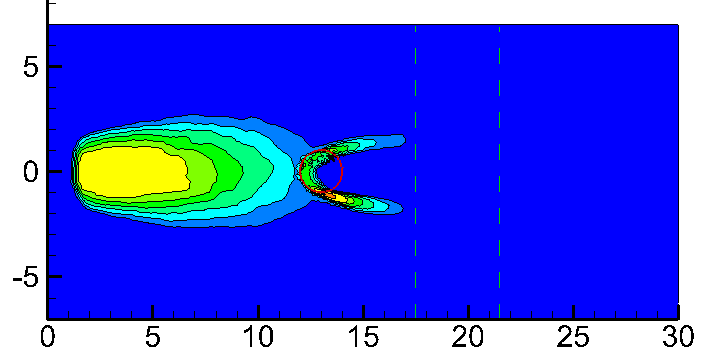 Figure 32
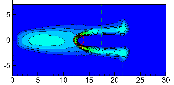 Figure 33
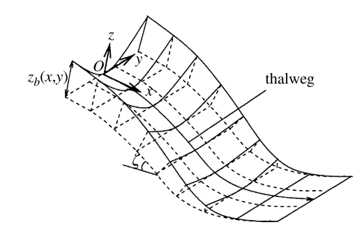 Figure 34
Peer Reviews
No public reviews on file for this paper yet. If you reviewed it on a platform where reviews are public (OpenReview, ICLR, NeurIPS, ICML), you can paste yours below so the community can read it here.
Videos
No videos yet. Explain this paper in a talk, walkthrough, or lecture? Add one.
Taxonomy
TopicsLandslides and related hazards · Cryospheric studies and observations · Fluid Dynamics and Turbulent Flows
A Finite Volume Scheme for
Savage-Hutter Equations on Unstructured Grids
Ruo Li
CAPT, LMAM and School of Mathematical Sciences, Peking University, Beijing 100871, P.R. China
and
Xiaohua Zhang
College of Science and Three Gorges Mathematical Research Center, China Three Gorges University, Yichang, 443002, China
Abstract.
A Godunov-type finite volume scheme on unstructured triangular grids is proposed to numerically solve the Savage-Hutter equations in curvilinear coordinate. We show the direct observation that the model is a not Galilean invariant system. At the cell boundary, the modified Harten-Lax-van Leer (HLL) approximate Riemann solver is adopted to calculate the numerical flux. The modified HLL flux is not troubled by the lack of Galilean invariance of the model and it is helpful to handle discontinuities at free interface. Rigidly the system is not always a hyperbolic system due to the dependence of flux on the velocity gradient. Even though, our numerical results still show quite good agreements to reference solutions. The simulations for granular avalanche flows with shock waves indicate that the scheme is applicable.
keywords: granular avalanche flow, Savage-Hutter equations, finite volume method, Galilean invariant
1. Introduction
The Savage-Hutter model was first proposed to describe the motion of a finite mass of granular material flowing down a rough incline, in which the granular material was treated as an incompressible continuum [25, 7, 11]. It was then extended to 2D and with curvilinear coordinate [10, 9, 8] which may be applied to study natural disasters as landslides and debris flows [18]. For more details on Savage-Hutter model, we refer to [11, 23, 6, 12, 13, 22].
Numerical method for the Savage-Hutter model may be dated back to work in [25, 15] using finite difference methods which are not able to capture shock waves. Later on, regardless of the Savage-Hutter model or other avalanches of granular flow models, the Godunov-type schemes are commonly used in literature [4, 29, 1, 2, 30, 28, 24] considering that most of them have hyperbolic nature of the depth averaged equations. We note that rigidly, the Savage-Hutter model is not hyperbolic since its flux is depended on the gradient of velocity. Precisely, the dependence is on the sign of the gradient of velocity components, that the model does be hyperbolic in the region with monotonic velocity components. Some related interesting development on numerical methods can be found in such as [27, 19, 1, 20, 17].
In practical scenario, landslides, rock avalanches and debris flows usually occur in mountainous areas with complex topography, that we have to use unstructured grids for numerical simulation. However, there is few work of numerical methods for Savage-Hutter equations on unstructured grids. This may due primarily to the lack of Galilean invariance of the model, which is a direct observation to the model as we point out in section 2. In this paper, we are motivated to develop a high resolution and robust numerical model for Savage-Hutter equations under the unstructured grids. Whether the numerical method may provide a correct solution on the unstructured grids for a problem without Galilean invariance is a major question here. Meanwhile, the loss of hyperbolicity at the zeros of velocity gradients may some unpredictable behavior in numerical solutions, too.
Additionally, there are still some challenges in numerical solving strongly convective Savage-Hutter equations on unstructured grids. For example, shock formation is an essential mechanism in granular flows on an inclined surface merging into a horizontal run-out zone or encountering an obstacle when the velocity becomes subcritical from its supercritical state [29]. Therefore, numerical efficiency is an important issue to help resolve the steep gradients and moving fronts. Noticing that the Savage-Hutter equations and Shallow water equations have some similarities, we basically follow the method in [3] for shallow water equations. The modified HLL flux is adopted to calculate the numerical flux on the cell boundary. The formation of the modified HLL flux does not require the flux to be Galilean invariant, thus formally we have no difficulties in calculation of numerical flux. The techniques involved to improve efficiency include the MUSCL-Hancock scheme in time discretization, the ENO-type reconstruction and the -adaptive method in spatial discretization.
We apply the numerical scheme to three examples. The first one is a granular dam break problem, and the second one is a granular avalanche flows down an incline plane and merges continuously into a horizontal plane. In the third example, a granular slides down an inclined plane merging into a horizontal run-out zone is simulated, whereby the flow is diverted by an obstacle which is located on the inclined plane. It is interesting that in these examples, the numerical solutions are agreed with the references solutions quite well. We are indicated that the scheme is applicable to the model, though the model is lack of the Galilean invariance and is not always hyperbolic. The reason why the loss of the hyperbolicity of the model are not destructive to the numerical methods is still under investigation.
The rest part of the paper is organized as follows. In section 2, the Savage-Hutter equations on the curivilinear coordinate is briefly introduced. We directly show that the system is not Galilean invariant. In section 3, we give the details of our numerical scheme. In section 4, we present the numerical results and a short conclusion in section 5 close the paper.
2. Governing Equations
There are various forms of Savage-Hutter equations according to different coordinate system and a detailed derivation of these different versions of Savage-Hutter equations has been given in [23]. Here, we confine ourselves to one of them. Precisely, the governing equations are built on an orthogonal curvilinear coordinate system (see Fig. 1) given in [1]. The curvilinear coordinate is defined on the reference surface, where the -axis is oriented in the downslope, the -axis lies in the cross-slope direction of the reference surface and the -axis is normal to them. The downslope inclination angle of the reference surface only depends on the downslope coordinates , that is, there is no lateral variation in the -direction, thus it is strictly horizontal. The shallow basal topography is defined by its elevation above the curvilinear reference surface.
The corresponding non-dimensionless Savage-Hutter equations are
[TABLE]
[TABLE]
[TABLE]
where is the avalanche depth in the direction, and are the depth-averaged velocity components in the downslope() and cross-slope() directions, respectively. The factors , are defined as
[TABLE]
respectively, where is aspect ratio of the characteristic thickness to the characteristic downslope extent. Here , are the , directions earth pressure coefficients defined by the Mohr-Coulomb yield criterion. Generally, the earth pressure coefficients are considered in the active or passive state, which depends on whether the downslope and cross-slope flows are expanding or contracting [21]. Hutter et al. assumed that , link the normal pressures in the , directions with the overburden pressure and suggested that [26, 10]
[TABLE]
[TABLE]
where and are the internal and basal Coulomb friction angles, respectively. The subscripts “act” and “pass” denote active(“”) and passive (“”) stress by
[TABLE]
[TABLE]
In this model the earth pressure coefficients , are assumed to be functions of the velocity gradient.
The terms , are the net driving accelerations in the , directions, respectively,
[TABLE]
[TABLE]
where , is the local curvature of the reference surface, and is the local stretching of the curvature.
The two dimensional Savage-Hutter equations (1)-(3) can be collected in a general vector form as
[TABLE]
where denotes the vector of conservative variables, represent the physical fluxes in the and directions, respectively, and is the source term. They are
[TABLE]
The flux for (4) and (5) along a direction is , while is a unit vector. The Jacobian of the flux along is given by
[TABLE]
where and are the components of the unit vector in the and directions, respectively. The three eigenvalues of the flux Jacobian are
[TABLE]
where .
For laboratory avalanches, the ranges of and are usually made and greater than zero [11, 23], thus, the eigenvalues of the flux Jacobian are all real and are distinct if the avalanche depth . Therefore the Savage-Hutter system given by (4) and (5) is hyperbolic if the gradient of velocity components are not zeros.
Clearly, the Savage-Hutter equations have a very similar mathematical structure to the shallow water equations of hydrodynamics at a first glance. But as a matter of fact, the derivation of Savage-Hutter equations are not the same as those in the shallow water approximation although they both start from the incompressible Navier-Stokes equation. Meanwhile, on account of the jump in the earth pressure coefficients and , the complex source term and , the free surface at the front and rear margins, it can be quite complicated to develop an appropriate numerical method to solve the Savage-Hutter equations.
It is a direct observation that the Savage-Hutter equations is not Galinean invariant. Precisely, it is not rotational invariant if . It is well-known that the shallow water equations is rotational invariant. This is an essential difference between the shallow water equations and the Savage-Hutter equations. Let us point out this fact by
Theorem 1**.**
For any unit vector , , and all vectors , the following equality
[TABLE]
holds if and only if , where the rotation matrix is as
[TABLE]
Proof.
First we calculate . The result is
[TABLE]
Next we compute and obtain
[TABLE]
Then we apply the inverse rotation to and get
[TABLE]
For the left hand of Eq. (6), we have
[TABLE]
Thus, if , (7) is not equal to (8). ∎
If the system is rotational invariant, one may solve a 1D Riemann problem with , where , as variable and get a 1D numerical flux , then the numerical flux along for 2D problem is given as . This procedure is very popular while it only works in case that holds. The theorem tells us that this equality holds only when or . In a finite volume method to be investigated, will be set as the unit normal of the cell interfaces, that it can not always vanish in unstructured grids. Therefore, if , any approximate Riemann solver based on such a procedure is out of the scope of our candidate numerical flux.
3. Numerical Method
Let us discretize the Savage-Hutter equations (4) and (5) on the Delaunay triangle grids using a finite volume Godunov-type approach. We will adopt the modified HLL approximate Riemann Solver to calculate numerical fluxes across cell interfaces. The MUSCL-Hancock method and ENO-type reconstruction technique are adopted to achieve second-order accuracy in space and time.
3.1. Finite volume method
Before introducing the cell-centered finite volume method, the entire spatial domain is subdivided into triangular cells . In each cell , the conservative variables of Savage-Hutter equations are discretized as piecewise linear functions as
[TABLE]
where is the cell average value, is the slope on and is the barycenter of , the superscript indicates at time .
To introduction the finite volume scheme, Eq. (4) is integrated in a triangle cell
[TABLE]
Applying Green’s formulation, Eq.(9) becomes
[TABLE]
where denotes the boundary of the cell ; is the unit outward vector normal to the boundary; is the arc elements. The integrand is the outward normal flux vector in which . Define the cell average:
[TABLE]
where is the area of the cell . The method achieves second-order accuracy by using the MUSCL-Hancock method which consists of predictor and corrector steps. The procedure of the predictor-corrector Godunov-type method goes as follows:
Step 1: Predictor step
[TABLE]
where is the -th edge of with the unit outer normal as , and is source term discretized by a centered scheme. The flux vector is calculated at each cell face after ENO-type piecewise linear reconstruction. is the time step.
Step 2: Corrector step
[TABLE]
where the numerical flux vector is evaluated based on an approximate Riemann solver at each quadrature point on the cell boundary. In the paper, we use HLL approximate Riemann solver owe to its simplicity and stable performance on wet/day interface.
3.2. HLL approximate Riemann solver
For a lot of hyperbolic systems, it uses the approximate Riemann solvers to obtain the approximate solutions in most practical situations. Since Savage-Hutter equations and shallow water equations are very similar, we can directly extend approximate Riemann solvers of shallow water equations to Savage-Hutter equations. The HLL approximate Riemann solver can offer a simple way of dealing with dry bed situaitons and the determination of the wet/dry front velocities [5]. Similar to shallow water equations, the numerical interface flux of HLL for Savage-Hutter equations is computed as follows
[TABLE]
where and are the left and right Riemann states for a local Riemann problem, respectively. and are estimate of the speeds of the left and right waves, respectively. The key to the success of the HLL approach is the availiability of estimates for the wave speeds and . For the Savage-Hutter equations, there are also dry/wet bed cases. Thus, in order to take the dry bed into account, similar to shallow water equations, the left and right wave speeds are expressed as
[TABLE]
[TABLE]
where , , , and
[TABLE]
3.3. Linear reconstruction
In order to get second order accuracy in spatial, a simple ENO-type piecewise linear reconstruction was applied to suppress the numerical oscillations near steep gradients or discontinuites. This reconstrction method had been used by Deng et. al. for shallow water equations [3].
This part is mainly taken from [3]. For a variable or , assuming its cell average value on is given (see Fig. 2), then we can get the gradients of for the three triangles , and are referred to as , and , and choose the one with the minimal norm as , that is,
[TABLE]
Acoording to the idea of minmod slope limiter, we let when or . Meanwhile, in the process of reconstructing , we must consider the physical criteria, that is, the avalanche depth must be non-negative at each quadrature points, otherwise is set to be zero.
3.4. Time stepping
The time-marching formula is explicit, and the time step length is determined by the Courant-Friedrichs-Lewy(CFL) condition for its stability. For triangular grid and implemention of CFL condition, the time step length is usually expressed as
[TABLE]
where is the Courant number specified in the range , and is adopted in our simulations; , is the total number of cells, and is the size of . For triangular grid, is usually calculated as the minimum barycenter-to-barycenter distance between and its adjacent cells.
4. Numerical Examples
In this section, three numerical examples were performed to verify the proposed scheme which implemented using C++ programming language based on the adaptive finite element package AFEPack[16]. The initial triangular grids were generated by easymesh. Because the posteriori error estimator for -adaptive method on unstructured grid was not the main goal of this work, we just applied the following local error indicator which advised by [3]
[TABLE]
where
[TABLE]
in which is a cell in the mesh and is its area, denotes the jump of a variable across , and is the piecewise linear numerical solution for , respectively.
4.1. Dam break test cases with exact solution
For this dam break problem, it was originally a one dimensional problem with analytical solutions involving a constant bed slope and a Coulomb frictional stress, thus, its governing equations can reduced as [14][30]
[TABLE]
where is the gravitational constant, the analytical solution of a granular dam break problem is given [30]:
[TABLE]
where and
[TABLE]
[TABLE]
In order to check the performance of the numerical schemes proposed in this work, we modified it to an equivalent two-dimensional problem as Ref.[30]. The computational domain is , the initial conditions are
[TABLE]
and .
Fig. 3 plots the compute avalanche depth in comparison with the exact solutions at and . It can be seen that our numerical solutions are in agreement with exact solutions very well, which also verifies the robustness and validity of our numerical algorithm.
4.2. Avalanche flows slide down an inclined plane and merge
continuously into a horizontal plane
In this section, we simulate an avalanche of finite granular mass sliding down an inclined plane and merging contiuously into a horizontal plane, which was considered in [29] to verify their model’s ability.
In order to compare with the results from Ref. [29][30], all computational parameters are set to the same as they are. That is, the computational domain is , and in our simulations. The inclined section lies and the horizontal region lies with a smooth transition zone lies . The inclination angle is given by
[TABLE]
where and . The granular mass is suddenly released at from the hemispherical shell with an initial radius of in dimensionless length units. The center of the cap is initially located at .
Fig. 4 shows the avalanche depth contours of the fluid at eight time slices as the avalanche slides on the inclined plane into the horizontal run-out zone. From the Fig. 4 it can be seen that, the avalanche starts to flow along the and direction due to gravity, and it flows faster along the downslope direction obviously. At the part of granular reaches the horizontal run-out zone and begins to deposite because of the basal friction is sufficient large, and the tail is still doing the acceleration movement. Here, some small numerical oscillations are visible in the solutions which also found in Ref.[29][30] with orthogonal quadrilateral mesh. At a shock wave develops round the end of the transition zone at and a surge wave is created. During the to , most of graunlar mass are accumulated at the end of the transition zone and the front-end of the horizontal zone, meanwhile, a obvious backward surge can be found. At the final deposition of the avalanche is nearly formed and an expansion fan is observed.
On the whole, our numerical resluts are identical with these available from Ref. [29][30]. Fig. 5 presents the mesh adaptive moving for the avalanche granular flows down the inclined plane and merges contiuously into a horizontal plane at . It can be seen that the triangle mesh is refined at the free surface where gradients varied significantly.
4.3. Granular flow pasts obstacle
The research of granular avalanches around obstacle is of partiacular interest because some important pheomena such as shock waves, expansion fans and granular vacuum can be observed [2]. Meanwhile, setting obstacles is an effective means to control the dynamic process of granular avalanche flow. In this section, we present a simulation example of finite granular mass flows down an inclined plane and merges inito a horizontal run-out zone with a conical obstacle located on the inclined plane. In addition, in order to compared the effects of with and without obstacle, all compuational parameters (such as computational domain, the inclination angle , , ) are the same as the above example. A conical obstacle is incorporated into this model and the centre of obstacle is located at with dimensionless radius of bottom-circle of 1 and dimsionless heights .
Fig. 6 shows a series of snap-shots of the thickness contours as the avalanche slides down the inclined plane which has a conical obstacle in the avalanche track. It can be seen that the flow of granular is the same as that without obstacle before it reaches the obstacle (eg. for ). At the granular avalanche has reache the obstacle, some of them climb the obstacle, and the other divide into two parts and flow around the obstacle downwards. At the moment, a stationary zone appears in the front of the obstacle, where the avalance velocity becomes zero, but it is followed by a great increase in the avalanche thickness. Meanwhile, behind the obstacle, a so-called granular vacuum is formed which can protect the zone directly behind it from disasters. At , the granular mass continues to accelerate until it reaches the horizontal run-out zone where the basal friction is sufficient large, which results in the front becomes to rest, but the part of the tail accelerates further. At the shcoks waves fromed on the horizontal run-out zone during the front of granular mass deposits and the tail of it still slides accelerated. From to , most of the granualr mass has slided down either side of the obstacle and on the transition zone two expansion fans gradually formed. For two separate and symmetrical deposition mass of granular are formed at the end of transition zone and the front of horizontal zone. From to there always has the flow-free region directly behind the obstacle, which can be regarded as the protected area in the practial application of avalanche protection. Thus, the obstacle does change the path of granular avalanche flow movement and affects its final deposition pattern. The numerical results show that our numerical model has the ability of capturing key qualitative features, such as shocks wave and flow-free region. As in the previous example, Fig. 7 also shows the adaptive mesh moving for the granular avalanche flows down with a obstacle at .
5. Conclusions
This paper is an attempt to solve the Savage-Hutter equations on unstructred grids. Keeping in mind that the model is not rotational invariant, it is more than encouraging for our numerical scheme to attain numerical results with good agreement to the reference solutions. It is indicated that the method is applicable to problems as granular avalanche flows. The underlying reason why the scheme works smoothly is still under investigation.
Acknowledgement
This work is financially supported by the National Natural Science Foundation of China(No. 11826207 and No. 11826208).
The reference list from the paper itself. Each links out to its DOI / PubMed record.
- 1[1] M. C. Chiou, Y. Wang, and K. Hutter. Influence of obstacles on rapid granular flows. Acta Mechanica , 175:105–122, 2005.
- 2[2] X. Cui. Computational and experimental studies of rapid free-surface granular flows around obstacles. Computers and Fluids , 89:179–190, 2014.
- 3[3] Jian Deng, Ruo Li, Tao Sun, and Shuonan Wu. Robust a simulation for shallow flows with friction on rough topography. Numerical Mathematics: Theory, Methods and Applications , 6(2):384–407, 2013.
- 4[4] Roger P. Denlinger and Richard M. Iverson. Flow of variably fluidized granular masses across three-dimensional terrain: 2. Numerical predictions and experimental tests. Journal of Geophysical Research: Solid Earth , 106:553–566, 2001.
- 5[5] Luigi Fraccarollo and Eleuterio F. Toro. Experimental and numerical assessment of the shallow water model for two-dimensional dam-break type problems. Journal of Hydraulic Research , 33:843–864, 2010.
- 6[6] J. M.N.T. Gray. Granular flow in partially filled slowly rotating drums. Journal of Fluid Mechanics , 441:1–29, 2001.
- 7[7] J. M.N.T. Gray, Y. C. Tai, and S. Noelle. Shock waves, dead zones and particle-free regions in rapid granular free-surface flows. Journal of Fluid Mechanics , 491:161–181, 2003.
- 8[8] J. M.N.T. Gray, M. Wieland, and K. Hutter. Gravity-driven free surface flow of granular avalanches over complex basal topography. Proceedings of the Royal Society of London. Series A: Mathematical, Physical and Engineering Sciences , 455:1841–1874, 1999.