Collision of two kinks with inner structure
Yuan Zhong, Xiao-Long Du, Zhou-Chao Jiang, Yu-Xiao Liu, Yong-Qiang, Wang

TL;DR
This paper investigates the collision dynamics of kinks with inner structure in a scalar field model, revealing complex behaviors and dependencies on model parameters through numerical simulations.
Contribution
It introduces a scalar field model with scalar-kinetic coupling supporting structured kinks and explores their collision outcomes and parameter dependencies.
Findings
Critical velocity varies with model parameters.
Presence of two-bion escape states.
Complex collision phenomena like intertwined states.
Abstract
In this work, we study kink collisions in a scalar field model with scalar-kinetic coupling. This model supports kink/antikink solutions with inner structure in the energy density. The collision of two such kinks is simulated by using the Fourier spectral method. We numerically calculate how the critical velocity and the widths of the first three two bounce windows vary with the model parameters. After that, we report some interesting collision results including two-bion escape final states, kink-bion-antikink intermediate states and kink or antikink intertwined final states. These results show that kinks with inner structure in the energy density have similar properties as those of the double kinks.
Click any figure to enlarge with its caption.
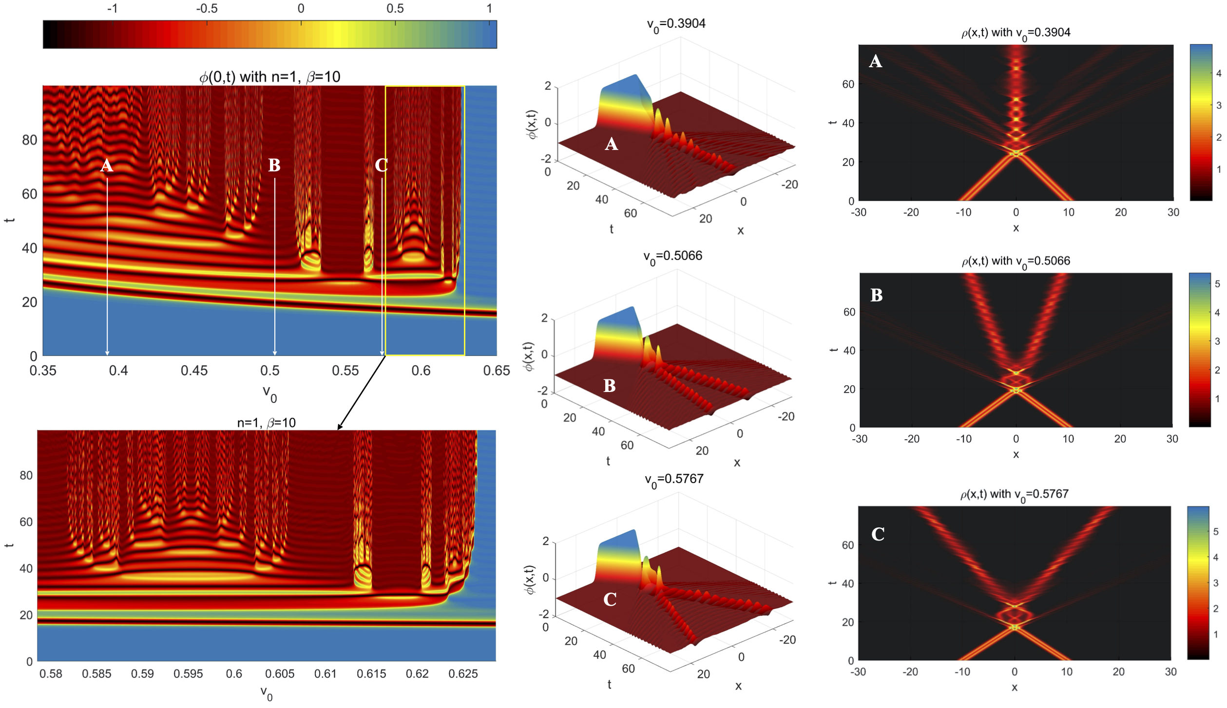 Figure 1
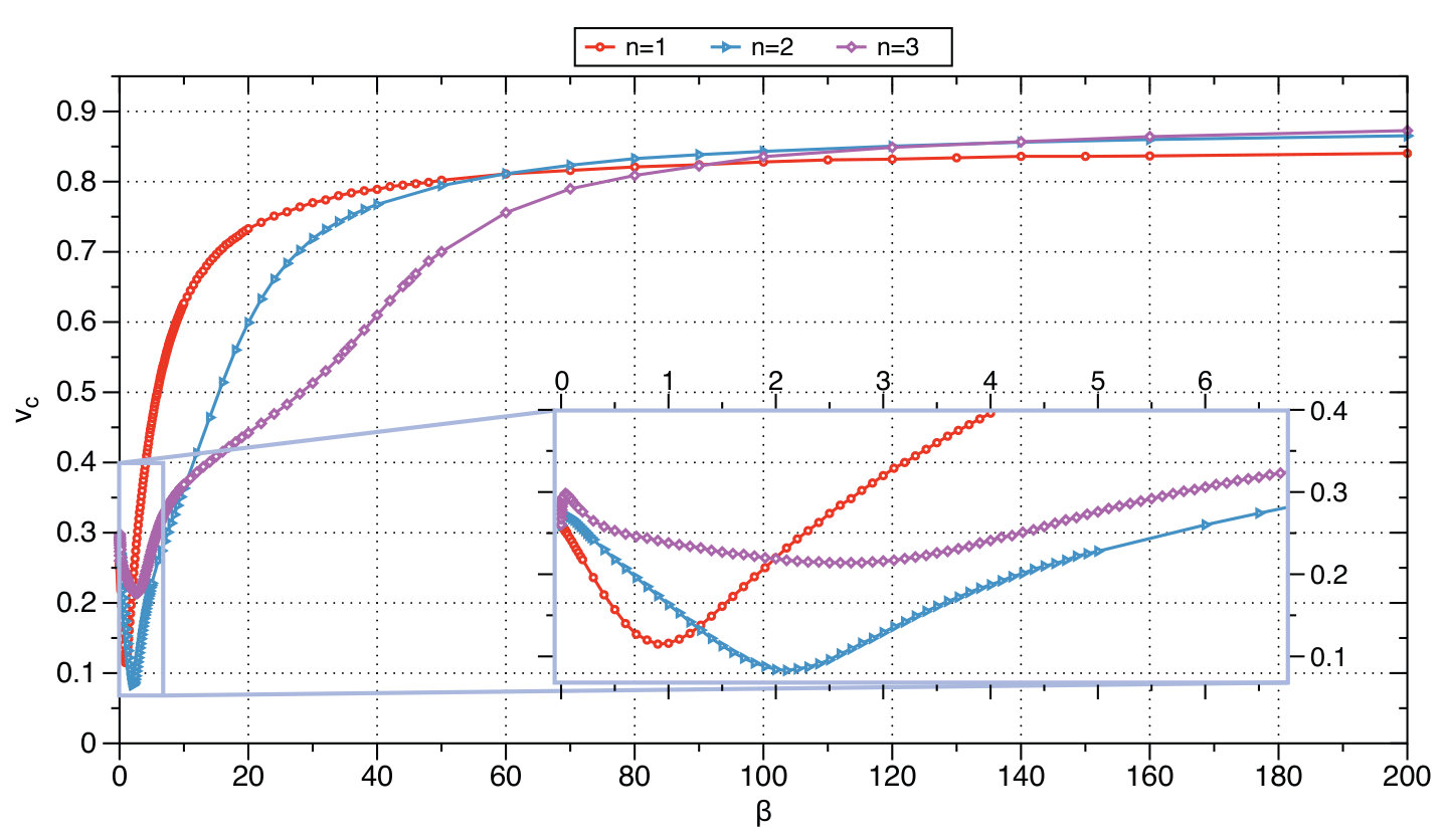 Figure 2
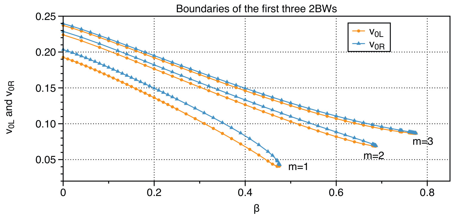 Figure 3
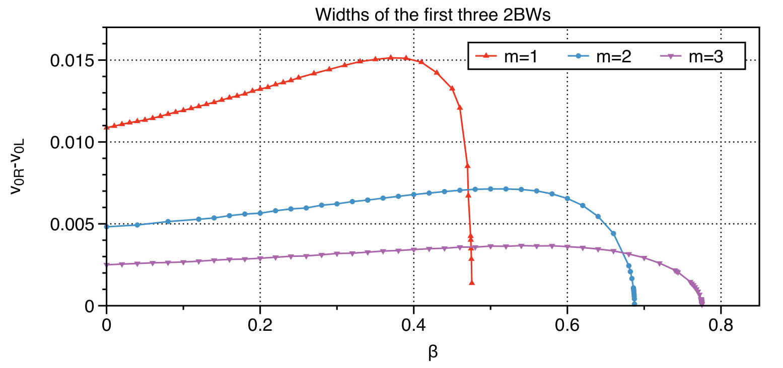 Figure 4
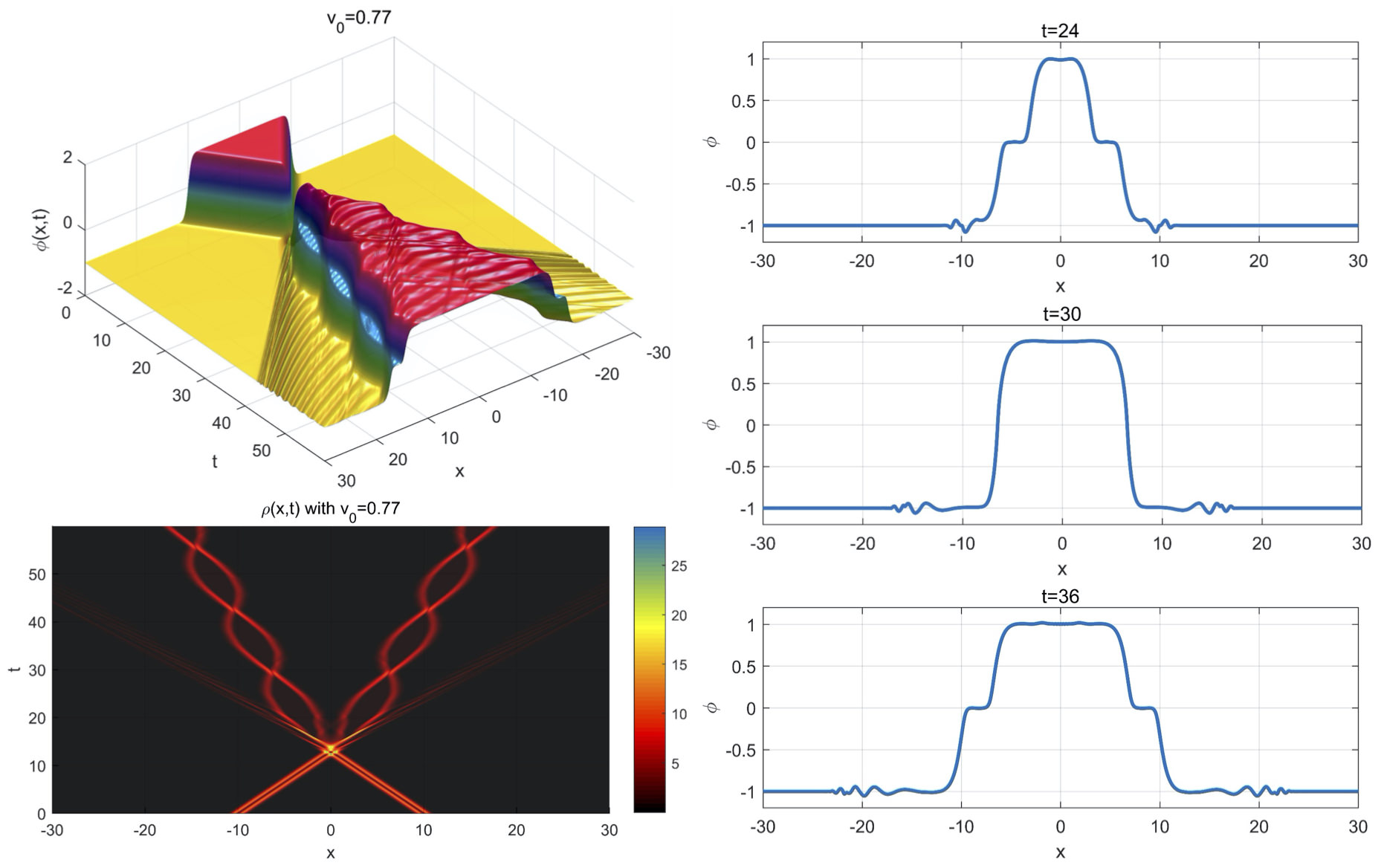 Figure 5
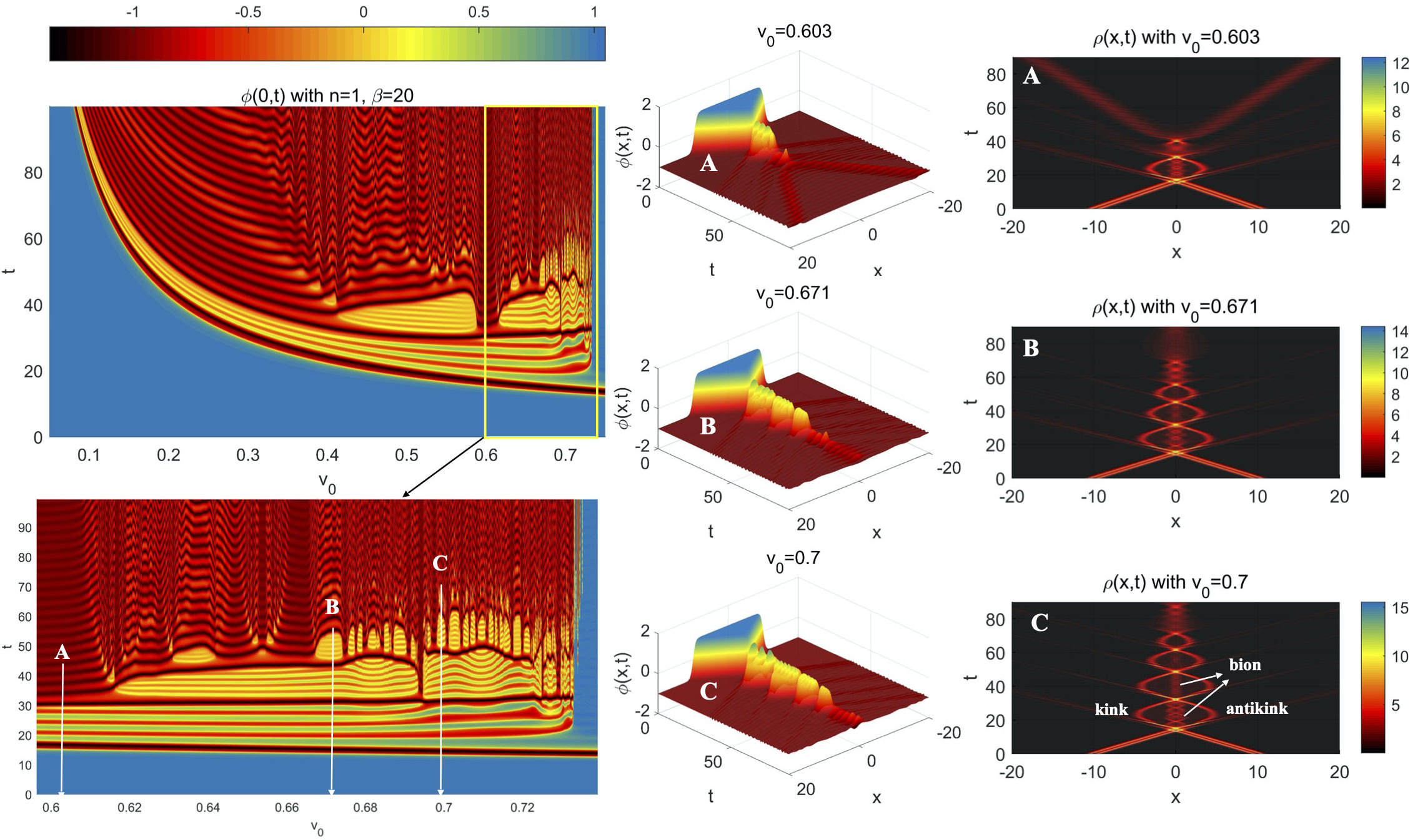 Figure 6
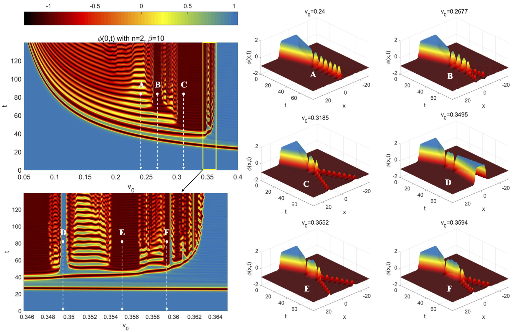 Figure 7
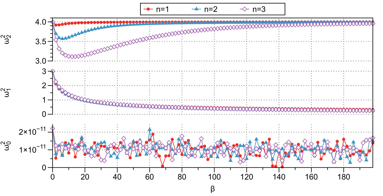 Figure 8
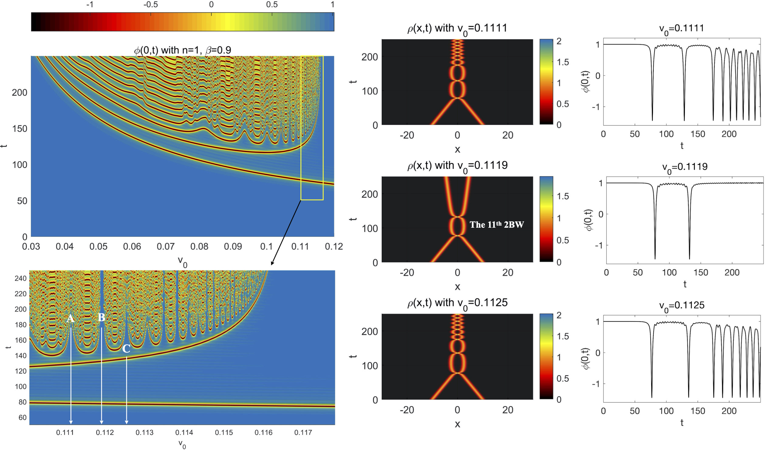 Figure 9
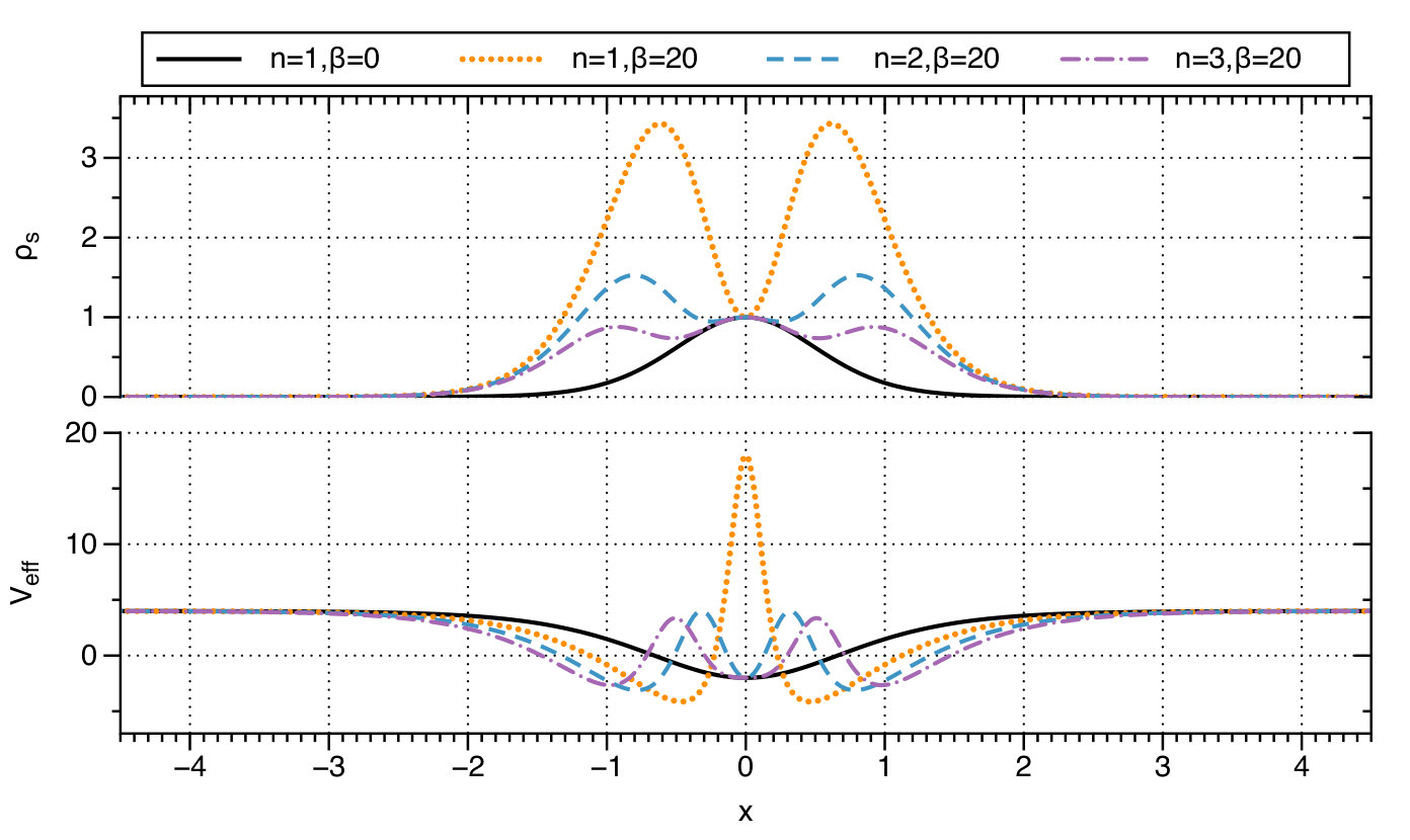 Figure 10
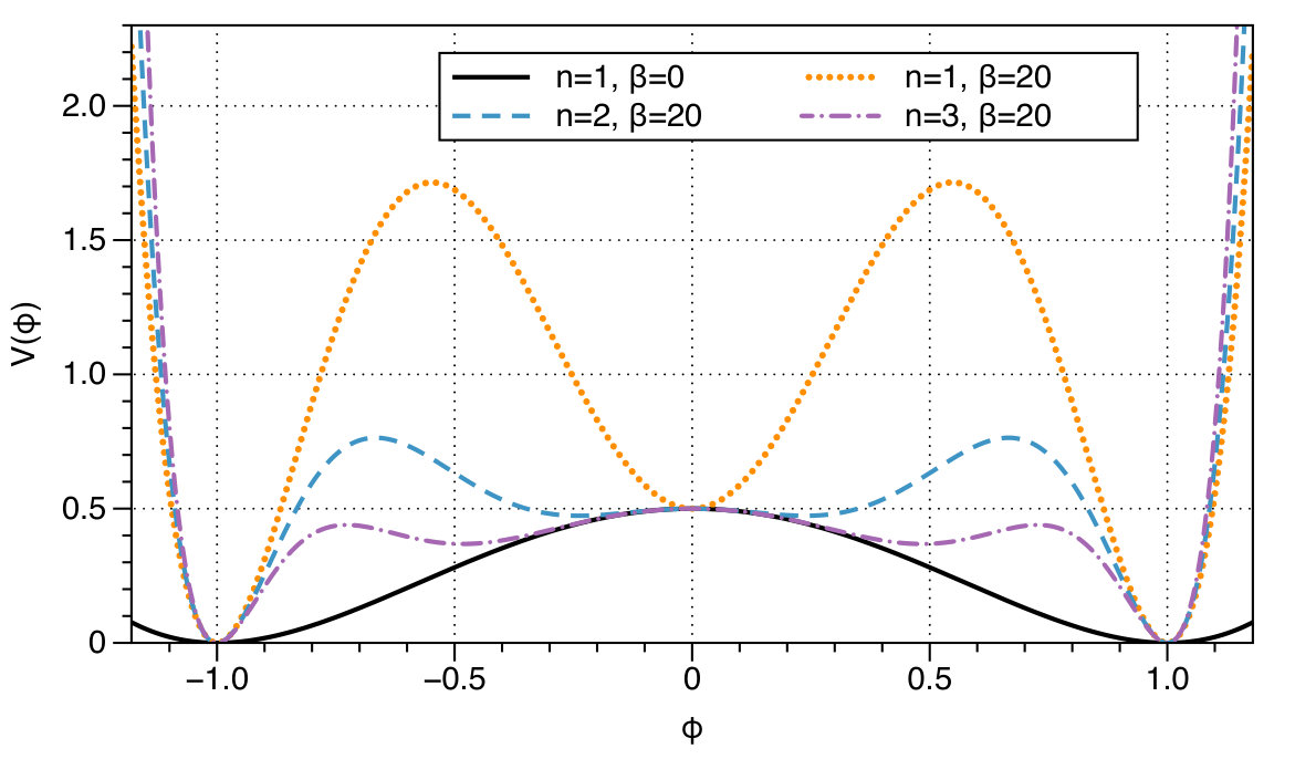 Figure 11
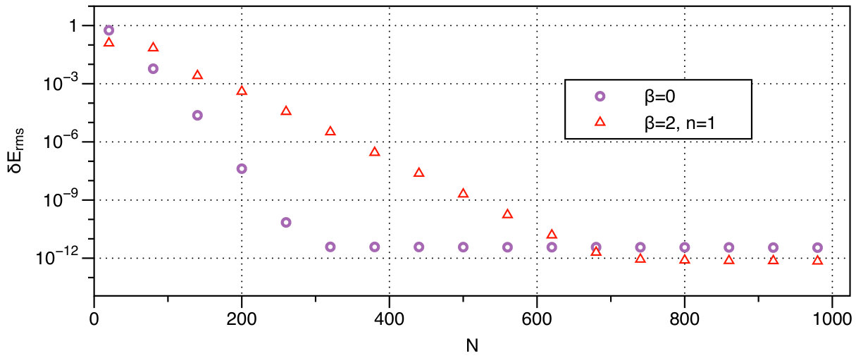 Figure 12
| — | (0.04, 0.2711) | (0.04, 0.2982) | |
| (0.9, 0.115) | (2.1, 0.083) | (2.8, 0.214) |
Peer Reviews
No public reviews on file for this paper yet. If you reviewed it on a platform where reviews are public (OpenReview, ICLR, NeurIPS, ICML), you can paste yours below so the community can read it here.
Videos
No videos yet. Explain this paper in a talk, walkthrough, or lecture? Add one.
aainstitutetext: School of Science, Xi’an Jiaotong University, Xi’an 710049, People’s Republic of Chinabbinstitutetext: Carnegie Observatories, 813 Santa Barbara Street, Pasadena, CA 91101, USAccinstitutetext: Institute of Theoretical Physics & Research Center of Gravitation, Lanzhou University, Lanzhou 730000, People’ s Republic of China
Collision of two kinks with inner structure
Yuan Zhong b
Xiao-Long Du a
Zhou-Chao Jiang c
Yu-Xiao Liu111Corresponding author. c
Yong-Qiang Wang
Abstract
In this work, we study kink collisions in a scalar field model with scalar-kinetic coupling. This model supports kink/antikink solutions with inner structure in the energy density. The collision of two such kinks is simulated by using the Fourier spectral method. We numerically calculate how the critical velocity and the widths of the first three two bounce windows vary with the model parameters. After that, we report some interesting collision results including two-bion escape final states, kink-bion-antikink intermediate states and kink or antikink intertwined final states. These results show that kinks with inner structure in the energy density have similar properties as those of the double kinks.
Keywords:
soliton, domain walls and instantons
††arxiv: 1906.02920
1 Introduction
Kinks are topological defects in dimensional space-time, and have been applied in many areas of physics Rajaraman1982 ; Vachaspati2006 . An important and interesting topic in the study of kinks is the interaction between kinks and antikinks. In integrable models, such as the sine-Gordon model, kink and antikink can pass each other after the collision with at most a phase shift Das1989 . While in non-integrable models, the outcomes are more complex and sensitively depend on the initial velocities of kinks. Taking the model as an example, there exists a critical velocity Sugiyama1979 . When two kinks collide with a high initial velocity , they simply bounce back after a collision; while when , they form a bound state called bion (also known as oscillon) Kudryavtsev1975 . Interestingly, in some intervals of velocity below , instead of forming bion, kink and antikink finally escape after a finite number of collisions. These velocity intervals are called -bounce windows (BWs), if kinks collide times before bouncing back Moshir1981 ; CampbellSchonfeldWingate1983 . All the bounce windows together form a fractal-like structure AnninosOliveiraMatzner1991 ; GoodmanHaberman2007 . When generalized to higher dimensions, kinks can either describe a braneworld that we are living on RubakovShaposhnikov1983 , or a bubble that we are living inside KobzarevOkunVoloshin1975 ; Coleman1977 ; CallanColeman1977 . The collisions between both branes KhouryOvrutSteinhardtTurok2001 ; KalloshKofmanLinde2001 ; Linde2001 ; TakamizuMaeda2004 ; TakamizuMaeda2006 ; GibbonsMaedaTakamizu2007 ; TakamizuKudohMaeda2007 ; Maeda2008 ; OmotaniSaffinLouko2011 and bubbles HawkingMossStewart1982 ; GiblinHuiLimYang2010 ; ZhangPiao2010 ; AguirreJohnson2011 ; Kleban2011 ; WainwrightJohnsonPeirisAguirreEtAl2014 ; BondBradenMersini-Houghton2015 ; BradenBondMersini-Houghton2015 ; BradenBondMersini-Houghton2015a have been extensively investigated in the literature. More works on interaction of kinks can be found in refs. BelovaKudryavtsev1997 ; GoodmanHaberman2005 .
Recently, more and more researchers began to investigate kink interaction in other non-integrable models, such as models with higher-order polynomial potentials HoseinmardyRiazi2010 ; DoreyMershRomanczukiewiczShnir2011 ; Weigel2014 ; GaniKudryavtsevLizunova2014 ; GaniLenskyLizunova2015 ; Romanczukiewicz2017 ; BelendryasovaGani2017 ; SaxenaChristovKhare2018 ; GomesSimasNobregaAvelino2018 ; BelendryasovaGani2019 ; BazeiaMendoncaMenezesOliveira2019 , with various kinds of triangular potentials PeyrardCampbell1983 ; GaniKudryavtsev1999 ; SimasGomesNobregaOliveira2016 ; SimasGomesNobrega2017 ; GaniMarjanehAskariBelendryasovaEtAl2018 ; BazeiaBelendryasovaGani2018 ; BazeiaGomesNobregaSimas2019a ; BazeiaGomesNobregaSimas2019 , with generalized dynamics GomesMenezesNobregaSimas2014 , and with multi-component scalar fields AshcroftEtoHaberichterNittaEtAl2016 ; Alonso-Izquierdo2018b ; Alonso-Izquierdo2018 ; Alonso-Izquierdo2018a ; Alonso-IzquierdoBalseyroSebastianGonzalezLeon2018 ; Alonso-Izquierdo2019 ; Alonso-Izquierdo2019a .
Some of these works renewed our understanding towards bounce windows. For example, it has been widely accepted that in order to form bounce windows, a kink should have a vibrational mode. It is the resonant energy transition between the vibrational mode and the translational mode that causes the formation of bounce windows. This mechanism was proposed by Campbell, Schonfeld and Wingate CampbellSchonfeldWingate1983 , and has been successfully applied in many cases CampbellPeyrardSodano1986 ; KivsharFeiVazquez1991 ; ZhangKivsharVazquez1992 . But some recent works have shown that even there is no vibrational mode around a single kink, bounce windows can still be formed DoreyMershRomanczukiewiczShnir2011 ; GaniKudryavtsevLizunova2014 ; DoreyRomanczukiewicz2018 . On the other hand, more vibrational modes usually suppress the bounce windows SimasGomesNobregaOliveira2016 ; BazeiaGomesNobregaSimas2019 . The development of the collective coordinate method Weigel2014 ; TakyiWeigel2016 ; Weigel2018 and the discovery of the relation between bounce windows and the separatrix map GoodmanHaberman2005 also help us to understand the bounce window phenomenon.
Some other studies found that in higher-order models like , due to the long-range interactions between kinks MelloGonzalezGuerreroLopez-Atencio1998 ; GomesMenezesOliveira2012 ; KhareChristovSaxena2014 ; BelendryasovaGani2019 ; BazeiaMenezesMoreira2018 ; KhareSaxena2018 ; ChristovDeckerDemirkayaGaniEtAl2018 , the widely used superposition or production ansatz is problematic, and should be replaced by the so-called split-domain ansatz ChristovDeckerDemirkayaGaniEtAl2019 . The force between long-range interacting kinks has been calculated recently Manton2018 ; Manton2019 . There are also many other interesting topics on kink interaction, including multi-kink collision SaadatmandDmitrievKevrekidis2015 ; MarjanehSaadatmandZhouDmitrievEtAl2017 ; MarjanehGaniSaadatmandDmitrievEtAl2017 ; MarjanehAskariSaadatmandDmitriev2018 ; EkomasovGumerovKudryavtsevDmitrievEtAl2018 ; GaniMarjanehSaadatmand2019 , boundary scattering AntunesCopelandHindmarshLukas2004 ; ArthurDoreyParini2016 ; DoreyHalavanauMercerRomanczukiewiczEtAl2017 ; LimaSimasNobregaGomes2018 , negative radiation effect ForgacsLukacsRomanczukiewicz2008 ; YamaletdinovRomanczukiewiczPershin2019 , creating kink-antikink pair by colliding particles or wave packages DuttaSteerVachaspati2008 ; RomanczukiewiczShnir2010 ; DemidovLevkov2011a ; DemidovLevkov2011 ; DemidovLevkov2015 ; AskariSaadatmandDmitrievJavidan2018 , spectral walls AdamOlesRomanczukiewiczWereszczynski2019a ; AdamOlesRomanczukiewiczWereszczynski2019 . For more related works, see ref. RomanczukiewiczShnir2018a .
In this paper, we will consider the collision of two kinks with inner structure in the energy density. In some models, especially models with generalized dynamics, as the parameter varies, the energy density of the kink might split from one peak to multi peaks BazeiaLosanoMenezesOliveira2007 ; BazeiaLobaoMenezes2015a ; ZhongGuoFuLiu2018 . When this happens, we say that the kink possesses an inner structure. Kinks with inner structure are similar to, but essentially different from double kinks BazeiaMenezesMenezes2003 . Both structures have a local minimum at the center of the energy density function. But unlike the double kink case, where the local minimum at the center equals to zero, a kink with inner structure can have a nonzero local minimum at the center of the energy density function.
Collision between two double kinks was studied in many works, and some new interesting phenomena were found. For example, two-bion escape final states were found in double sine-Gordon model CampbellPeyrardSodano1986 ; GaniMarjanehAskariBelendryasovaEtAl2018 , and in sinh-deformed model BazeiaBelendryasovaGani2018 . Unstable kink-bion-antikink intermediate states were found in refs. MendoncaOliveira2015 ; MendoncaOliveira2015a .
In this work, we will consider a model with coupling between the scalar field and its kinetic term. Such a generalized dynamics enables the kink to have rich and tunable inner structures. We will study the collision between a kink and an antikink of this model. Our model and corresponding static kink solution will be given in the next section. The numerical simulation of kink collision will be conducted in section 3. Finally, we will end this paper by a conclusion and outlook in section 4.
2 The model, kink solution and its linear spectrum
In our model, the scalar field is coupled to its kinetic term via the following Lagrangian density:
[TABLE]
where . The parameter describes how much our model deviates from the canonical case (), while the parameter controls the number of local maxima in the energy density of the kink.
The equation of motion of our model is
[TABLE]
where the subscript denotes the derivative with respect to . A static solution can be obtained by solving the following equation:
[TABLE]
A powerful method for constructing analytical static kink solutions is the superpotential method BazeiaLosanoMenezes2008 ; ZhongLiu2014 , which begins with the assumption
[TABLE]
By integrating the equation of motion (3), one can find a simple relation between the scalar potential and the superpotential :
[TABLE]
where is an integral constant, which will be taken as zero.
The superpotential formalism (4)-(5) makes it easy to find static kink solutions. For example, by taking
[TABLE]
one immediately obtains the type kink solution
[TABLE]
Here, represents the vacuum expectation value of , and the width of the kink. In this work, we will focus on the collision of this type of kink solution, and always take for simplicity. Other solutions will be considered in our future works.
The scalar potential takes the following form
[TABLE]
which is not the standard double-well potential when , see fig. 1.
The energy density of our model takes the form
[TABLE]
In this work, we always use an overdot or a prime to denote the derivative with respect to time or space. For the static solution in eq. (7), the explicit expression of is
[TABLE]
whose shape is plotted in fig. 2. Obviously, splits if is large enough. Besides, the number of peaks of increases with for , and equals to three as . Unlike the case of double kink, where , the solution here always satisfies .
Another important property of the static kink solution is its linear spectrum. Consider a small linear perturbation around the background kink solution . Defining and , one may show that the equation for the perturbation to the first order is ZhongLiu2014
[TABLE]
We can expand with the Fourier modes
[TABLE]
where the mode functions satisfy a Schrödinger-like equation
[TABLE]
with the effective potential defined by
[TABLE]
The explicit expression of can be easily obtained after substituting in the kink solution. Here we only point out that when , its asymptotic behavior is , and its shape can be found in the lower panel of fig. 2.
The eigenvalues of the Schrödinger-like equation, , can be calculated numerically. In fig. 3, we plot the eigenvalues of all possible bound states for and . We find that in addition to the translational mode (the zero mode with frequency ), there are at most two vibrational modes, and , in the parameter ranges considered. For small , both and decrease as increases. But as becomes larger, and behave differently: the former keeps decreasing monotonically, while the later increases after reaching a local minimum.
3 Kink-antikink collision
In this section, we study the kink-antikink interaction. Since we have no analytical multikink solution of our model, we will solve the dynamical equation numerically by taking the widely used superposition ansatz as the initial condition
[TABLE]
Here is a kink initially located at and moving with an initial velocity of , and is the corresponding antikink solution. The solution of is obtained by simply boosting the static kink in eq. (7).
For simplicity, we will take periodical boundary condition, and solve the dynamical equation by using the Fourier spectral method. In this method, evenly spaced grid points, or collocation points, are chosen on a finite truncated space domain. The solution of the scalar field is approximated by a truncated Fourier series
[TABLE]
where the coefficients can be determined by requiring that at all collocation points. The -th order spatial derivative of the solution is then approximated by differentiating :
[TABLE]
Here is a constant matrix called the derivative matrix and we have used the fact that is a linear combination of at collocation points222The specific form of the derivative matrix can be found in Trefethen2001 ..
As a result, the original partial differential equation (PDE) (2) will be transformed into a system of second-order-in-time ordinary differential equations (ODEs), which can be easily solved by using the ode45 solver of Matlab (see also refs. Trefethen2001 ; ChristovDeckerDemirkayaGaniEtAl2018 ; ChristovDeckerDemirkayaGaniEtAl2019 ). The numerical precision of this method is determined by two factors: the spatial step size, which changes with the number of the collocation points ; and the time step size, which will be automatically determined by the ode45 solver in accordance with its step changing algorithm. To improve the precision, one could add more collocation points and tune the relative and absolute tolerance options of the ode45 solver333In Matlab, the default value of the relative and absolute tolerance of ode45 solver are RelTol= and AbsTol=. Usually, for a fixed number of collocation points , more precise solutions can be obtained by taking smaller RelTol and AbsTol..
To check the viability of our numerical results, we test the conservation of the total energy as the time evolution proceeded. For a single kink/anti-kink moving with velocity , the energy is
[TABLE]
Then, for a system of a pair of widely separated kink and anti-kink, the exact total energy is , which should be conserved all the time. We can compare our numerical solution with the exact one by defining the relative error of total energy at time as
[TABLE]
Because changes slightly with , it would be more convenient to use the root mean square error to estimate the long-term behavior of energy conservation. As examples, we consider two cases with and , respectively. The former case is just the standard model. For both cases we take and conduct simulations within the spatial domain for . As can be seen from fig. 4, converges exponentially as the collocation points increases, until it reaches the relative tolerance of the ode45 solver.
3.1 Critical velocity and two bounce windows
Our model reduces to the well studied model when . Therefore, it is interesting to see how a nonzero would change the well-known properties of the model. In this section, we will consider the impacts of and on the value of critical velocity and on the widths of the two bounce windows.
In fig. 5, we plot the critical velocity as a function of the parameter for cases with . For different values of , the global behavior of is similar: it has a global minimum around , and increases monotonically as . When , the critical velocity increases to about 0.85 for . It is also interesting to note that for , has a local maximum around , see table 1.
The model parameters also have impacts on the widths of the two bounce windows (2BWs). Figure 6 shows how the boundaries (the upper panel) and the widths (the lower panel) of the first three 2BWs (labeled by , respectively) vary with in the case with . As can be seen from the figure, when increases the 2BWs expand slightly at the beginning, then shrink rapidly, and finally close when is large enough. For , the first three 2BWs close at , respectively.
One may guess that, as increases further, the fourth, fifth 2BWs will close order by order. To test this, let us consider the case with . In order to get a global view on the collision results, we consider as a function of and . When is fixed, the function traces out a curve, which has many local minima with each corresponding to a collision of kinks (some examples can be found in the third column of fig. 7). While, if varies, the local minima form a complex pattern, from which we can easily see the distribution of BWs and bions. In figure, an BW is simply an interval of with dark lines.
In the first column of fig. 7, we plotted in the range and . The numerical calculation is conducted by setting the initial separation of the kinks as , and taking 400 collocation points in the domain . The tolerance option of ode45 solver is set as RelTol= and AbsTol=, which ensures that . From fig. 7, we can roughly estimate the value of critical velocity () and figure out the locations of 2BWs. For example, by magnifying the interval we find a clear 2BW around .
In the middle column of fig. 7, we plot the energy densities correspond to three different initial velocities: A , B and C . In the cases A and C, kinks collide many times at , which indicates the forming of bions. While in the case B, kinks only collide twice before escaping, and is a two bounce collision. From the figure of B, we clearly see that there are twelve local maxima between the two collisions, so B belongs to the 2BW. Point C locates at the center of the 2BW, which has been closed. So we can conclude that as increases further, the 2BWs do not closed order by order. We check these numerical results by taking collocation points.
3.2 Interesting intermediate and final states
In this section, we report some of the interesting phenomena in cases with large . For large , kinks can have rich structures in their energy densities. As we will see in this section, the collision of two kinks with inner structure can generate some interesting intermediate and final states.
One of the interesting phenomena is the escape of two bions, which has been found and discussed in many models such as the double Sine-Gordon model CampbellPeyrardSodano1986 ; GaniMarjanehAskariBelendryasovaEtAl2018 ; GaniMarjanehSaadatmand2019 , the sinh-deformed model BazeiaBelendryasovaGani2018 and other models with double kinks MendoncaOliveira2015 ; MendoncaOliveira2015a ; MendoncaDeOliveira2019 . In previous works, two-bion final states are usually generated by colliding a pair of double kinks. In this work, we find that when noncanonical dynamics is considered, it is also possible to generate two-bion escape final state from a kink-antikink initial state.
In figs. 8 and 9, we plot as a function of for and , respectively. For both cases, we can clearly see some two-bion escape windows. After magnification, narrower two-bion escape windows are found, just as higher-order bounce windows can be found by zooming in to the boundaries of any of the 2BWs. Especially, when two-bion escape windows coexist with a few 2BWs.
In addition to the two-bion escape windows, we also find some interesting intermediate states in the case with and . In fig. 10, we plotted in the range and . As can be seen from the figure, there are many yellow zones, each corresponds to a kink-bion-antikink intermediate state. Such state is constituted by a bion oscillating in the center and a kink and an antikink symmetrically moving away from the bion for a while and then come back to collide with the bion at . Such intermediate state has also been reported in a model with double kinks MendoncaOliveira2015 . In the range there is at least one such intermediate state, whose life time (the width of the lowest yellow zone) monotonically increases with . In some narrower windows of one may find three or even four (see point B and point C in fig. 10, respectively.) of such intermediate states after the collision of kinks.
The simulations of figs. 8-10 are conducted in spatial domain with firstly 600 and then checked with 1200 collocation points. The tolerance option of ode45 solver is set as RelTol= and AbsTol=. The relative error of energy is for , and for . The representative points A, B, are also checked by using more collocation points.
The above three case studies have shown that kinks with inner structure in their energy density can have similar properties as the double kinks. Now, let us report a novel phenomenon, namely, the kink intertwined final state. This phenomenon can be observed when is large enough and . As an example, we consider and . The evolution of the scalar field as well as the corresponding energy density can be found in fig. 11. We can see that in this case a new structure is formed after the kink-antikink collision. This structure is similar to bion in the sense that both of them are spatially localized oscillating solutions. The essential difference between them is that a bion is a bound state of a kink and an antikink, while the new structure we found here is a bound state of two kinks or two antikinks (see the right column of fig. 11). Another difference is that bion is formed at some initial velocities below , but the intertwined state of kinks can be formed only when .
We emphasize that neither the (anti-)kinks in the intermediate states nor those in the interwinded final states are the conventional ones, which connect two vacua . Instead, the (anti-)kinks in these states connect only one of the vacua with the local minimum at (see fig. 1).
4 Conclusion and outlook
In this work, we investigated the kink-antikink collision in a scalar field model with two free parameters and . When we come back to the model, while when , the energy densities of the kinks (antikinks) can have rich inner structure.
Before considering the collision of kinks, we first analyzed the linear spectrum of a static kink for and . We found that there are at most three bound states in this range of parameters. The first bound state is the zero mode with eigenvalue , which represents a translational mode. The second and the third bound states are two vibrational modes. As increases, the eigenvalue of the first vibrational mode monotonically decreases, while the second vibrational mode has a local minimum at . From fig. 3 we can see that and .
After the analysis of the linear structure, we began to consider how the parameters and would influence the well-known properties of model. We took the superposition of a kink and an antikink as the initial state, and then used the Fourier spectral method to simulate the kink-antikink collision numerically. We first calculated the critical velocity in the parameter scope and . We found that has a local minimum at . When , approaches to the speed of light .
Then we explored the impact of small on the width of the two bounce windows. For simplicity, we only considered the first three two bounce windows in the case with . We found that as increases, the two bounce windows first expand slightly and then shrink rapidly, and finally close at larger . We also pointed out that although the first three two bounce windows are closed order by order with the increase of , one cannot conclude that all the other two bounce windows are closed in this manner, as a counterexample has been found in the case with .
After this, we began to discuss the collision phenomena in the case with large . In this case the energy density of the kink can have more than one peak, and the kinks can have similar properties as those of the double kinks. For example, we have found many two-bion escape windows for and for . In the later case we also found the coexistence of two-bion escape windows and two bounce windows. For larger value of , for example in the case with we found the formation of some kink-bion-antikink intermediate states after the collision of kink and antikink. The number and the lifetime of these intermediate states depend on the incident velocity . This phenomenon can also be generated by colliding two double kinks MendoncaOliveira2015 .
Finally, we reported a novel bound state of two kinks or two antikinks. As an example, we considered the case with and , but one can also try many other values of parameters. Two basic requirements for finding this phenomenon are and .
This work revels the fact that kinks with inner structure in their energy density may have similar properties as those of the double kink solutions. Both can have two-bion escape final states and kink-bion-antikink intermediate states after a collision. When we found a new spatially localized oscillating structure, which to our knowledge, has not been reported before. Unlike the bion, which is a bound state of a kink and an antikink, the new structure we found here is a bound state between two kinks or two antikinks.
As an outlook, we would like to point out that we have not cover all the parameter ranges, for example, the cases with are not discussed. Even for we cannot claim that we have found all the distinct phenomena. As we have shown in subsection 3.2, the collision result sensitively depends on the values of and , but we have only studied a few representative values of . Therefore, it would be possible to find other new phenomena by considering different parameter settings from ours. Besides, the superpotential we taken in eq. (6) leads to a type of kink solution, it is easy to generate other kink (for example a sine-Gorden type of kink) or double kink solutions by simply taking different superpotentials. As a future direction, one can consider the collision of these kinks in our model. If one would like to go beyond the present model, there are many other noncanonical kink models such as those studied in refs. ZhongLiu2014 ; ZhongGuoFuLiu2018 . At present time, only a few works considered the interactions of noncanonical kinks GomesMenezesNobregaSimas2014 , so this field is worth further investigation. It is also interesting, despite challenging, to understand how the intermediate and final states we reported above are formed. Finally, it would be interesting to discuss the application of the intertwined two kink final states as a cosmological reheating mechanism, in parallel to the previous work TakamizuMaeda2004 .
Acknowledgment
This work was supported by the National Natural Science Foundation of China (Grant Numbers 11847211, 11605127, 11875151, 11522541, 11405121, and 11375075), the Fundamental Research Funds for the Central Universities (Grant No. xzy012019052), and by China Postdoctoral Science Foundation (Grant No. 2016M592770).
The reference list from the paper itself. Each links out to its DOI / PubMed record.
- 1(1) R. Rajaraman, Solitons and Instantons . North-Holland, Amsterdam, 1982.
- 2(2) T. Vachaspati, Kinks And Domain Walls . Cambridge University Press, 2006.
- 3(3) A. Das, Integrable Models . World Scientific Publishing Co. Pte. Ltd., 1989.
- 4(4) T. Sugiyama, Kink-antikink collisions in the two-dimensional ϕ 4 superscript italic-ϕ 4 \phi^{4} model , Prog. Theor. Phys. 61 (1979) 1550 . · doi ↗
- 5(5) A. E. Kudryavtsev, Solisoliton solutions for a higgs scalar field , JETP Lett. 22 (1975) 82.
- 6(6) M. Moshir, Soliton - Anti-soliton Scattering and Capture in λ ϕ 4 𝜆 superscript italic-ϕ 4 \lambda\phi^{4} Theory , Nucl. Phys. B 185 (1981) 318 . · doi ↗
- 7(7) D. K. Campbell, J. F. Schonfeld and C. A. Wingate, Resonance structure in kink-antikink interactions in ϕ 4 superscript italic-ϕ 4 \phi^{4} theory , Physica D: Nonlinear Phenomena 9 (1983) 1 . · doi ↗
- 8(8) P. Anninos, S. Oliveira and R. A. Matzner, Fractal structure in the scalar λ ( ϕ 2 − 1 ) 2 𝜆 superscript superscript italic-ϕ 2 1 2 \lambda(\phi^{2}-1)^{2} theory , Phys. Rev. D 44 (1991) 1147 . · doi ↗