Optimal Resource Procurement and the Price of Causality
Sen Li, Akhil Shetty, Kameshwar Poolla, Pravin Varaiya

TL;DR
This paper introduces the concept of the price of causality in resource procurement, quantifies it, and proposes algorithms and mechanisms for fair cost allocation in uncertain demand scenarios.
Contribution
It defines and analyzes the price of causality, providing bounds, exact calculations for special cases, and a fair cost allocation mechanism.
Findings
Upper bound on the price of causality established
Exact price computed for specific cases
Proposed mechanism is fair and budget-balanced
Abstract
This paper studies the problem of procuring diverse resources in a forward market to cover a set of uncertain demand signals . We consider two scenarios: (a) is revealed all at once by an oracle (b) reveals itself causally. Each scenario induces an optimal procurement cost. The ratio between these two costs is defined as the {\em price of causality}. It captures the additional cost of not knowing the future values of the uncertain demand signal. We consider two application contexts: procuring energy reserves from a forward capacity market, and purchasing virtual machine instances from a cloud service. An upper bound on the price of causality is obtained, and the exact price of causality is computed for some special cases. The algorithmic basis for all these computations is set containment linear programming. A mechanism is proposed to allocate the…
Click any figure to enlarge with its caption.
 Figure 1
 Figure 2
 Figure 3
 Figure 4
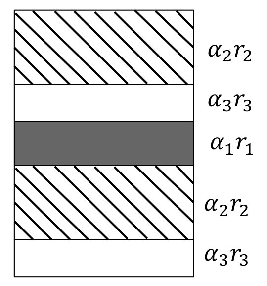 Figure 5
Peer Reviews
No public reviews on file for this paper yet. If you reviewed it on a platform where reviews are public (OpenReview, ICLR, NeurIPS, ICML), you can paste yours below so the community can read it here.
Videos
No videos yet. Explain this paper in a talk, walkthrough, or lecture? Add one.
Optimal Resource Procurement and
the Price of Causality
Sen Li†, Akhil Shetty⋆, Kameshwar Poolla⋆, and Pravin Varaiya⋆ This research is supported by the National Science Foundation under grants EAGER-1549945 and CPS-1646612, and by the National Research Foundation of Singapore under a grant to the Berkeley Alliance for Research in Singapore. The conference version of this paper was presented at 2018 European Control Conference [1]. †The Department of Mechanical Engineering, University of California, Berkeley, USA. Email: [email protected]⋆The Department of Electrical Engineering and Computer Science, University of California, Berkeley, USA. Email: {shetty.akhil, poolla, varaiya}@berkeley.edu
Abstract
This paper studies the problem of procuring diverse resources in a forward market to cover a set of uncertain demand signals . We consider two scenarios: (a) is revealed all at once by an oracle (b) reveals itself causally. Each scenario induces an optimal procurement cost. The ratio between these two costs is defined as the price of causality. It captures the additional cost of not knowing the future values of the uncertain demand signal. We consider two application contexts: procuring energy reserves from a forward capacity market, and purchasing virtual machine instances from a cloud service. An upper bound on the price of causality is obtained, and the exact price of causality is computed for some special cases. The algorithmic basis for all these computations is set containment linear programming. A mechanism is proposed to allocate the procurement cost to consumers who in aggregate produce the demand signal. We show that the proposed cost allocation is fair, budget-balanced, and respects the cost-causation principle. The results are validated through numerical simulations.
I Introduction
Many complex systems consist of both controllable and uncontrollable resources. Examples range from power systems, computing systems, transportation systems, among others. Uncontrollable resources inject uncertainties in the system, which collectively generate an uncertain demand signal that needs to be balanced by the controllable resources. We investigate optimal resource procurement necessary to balance the uncertain aggregate demand signal. One example is that of a grid operator that needs to procure energy reserves from the forward capacity market. He can choose from diverse resources, such as batteries, generators, aggregation of loads, etc. These resources are used to cover imbalances between electricity supply and demand for the grid. Another example is that of a company buying virtual machines from a cloud provider to serve computational demands, which are typically heterogeneous. The common thread that binds these examples is the ex-ante procurement of diverse resources to cover an uncertain signal revealed in real-time.
What is the optimal resource asset mix that covers all uncertain demand signals ? The purchase decision depends on the unit prices of the resources, their dynamic constraints, and critically on the control strategy that allocates the signal to the procured resources. The resource procurement decision is therefore intimately coupled with the real-time control strategy associated with allocation. Since the signal reveals itself in real-time, the allocation policy needs to be causal. The operator needs to irrevocably commit procured resources to match the uncertain demand without the luxury of knowing its future values. Clearly, the resource procurement cost under causal policies will be higher than that under arbitrary(possibly non-causal) policies. This inspires us to quantify the effect of causality on optimal resource procurement cost.
A second issue is that of paying for the procurement cost. Ideally, the cost allocation should be fair, budget-balanced, and follow the cost causation principle. This principle enunciates that agents are penalized (rewarded) in proportion to their contribution (mitigation) of the need to procure balancing resources. We explore cost allocation mechanisms that satisfy these requirements.
I-A Our Contribution
We formulate optimal resource procurement as a set containment problem. In particular, consider an operator that procures diverse resources to cover a sequence of uncertain signals revealed over a delivery window of length . Each resource has linear dynamic constraints, which can be modeled as a convex set in . Uncertain signals are modeled as belonging to a specified convex set . The operator needs to determine the optimal resource mix to collectively cover all signals in . The principle contributions of the paper are:
- •
We define the price of causality (PoC). It is the ratio of the optimal procurement cost under causal policies to that under arbitrary (possibly non-causal) policies. It quantifies the additional cost for not knowing the information in the future.
- •
We derive an upper bound on the price of causality. The algorithmic basis of this computation is set containment linear programming.
- •
We obtain the exact price of causality for some special cases. Through these cases, we show that dynamics and diversity are the main factors that drive the price of causality to be greater than 1.
- •
A cost allocation mechanism is proposed. It is fair, budget balanced, and respects the cost causation principle.
- •
We illustrate our framework in two application contexts: procuring energy reserves from forward capacity markets, and buying virtual machines from cloud providers.
I-B Related Work
A closely related problem is online optimization [2], [3]. It studies sequential decisions made irrevocably at each time step without access to future information. This problem is widely studied in many areas, such as stochastic dynamic programs [4], communication networks [5], online allocation [6], [7], load balancing [8], among others. A standard measure to evaluate the performance of an online solution is the competitive ratio [2]. This compares the performance of the optimal online algorithm, where all information is revealed causally, to the performance of the optimal offline algorithm, which is an unrealizable algorithm with complete information about the future. Online optimization problems consider the available resources to be fixed and aim to find the optimal causal decisions that minimize real-time costs. Our problem is distinct. We consider resource procurement problems that minimize ex-ante capacity cost. This distinction differentiates the price of causality from the competitive ratio.
Aside from online optimization, another strand of related work studies the adequacy of resources in real-time decision making. For instance, Dertouzos et al. studies the online processor time allocation problem in [9], and shows that optimal scheduling is impossible without a priori knowledge on the start times of tasks. Subramanian et al. considers a real-time scheduling problem for distributed energy resources to reduce the grid energy cost [10]. Wenzel et al. studies real-time charging strategies for electric vehicles to provide ancillary services with minimum tracking error [11]. Madjidian et al. discovers the trade-off between absorbing and releasing energy for collective loads under causal allocation policies [12]. In all of these works, the quantity of available resources is fixed. Their focus is on analysis of causal policies. In contrast, we investigate optimal resource procurement to meet worst case adequacy.
The closest related works are [13] and [14]. Negrete-Pincetic et al. considers a supplier who owns uncertain renewable generations and also purchases energy in day-ahead and real-time markets to serve the deferrable loads [14]. They show that the optimal procurement costs under causal allocation policy and offline allocation policy are the same, i.e., the price of causality is 1. In [13] and [14], the supplier can purchase additional energy from the real-time markets when the day-ahead procurement is not enough. This is distinct from our problem, where all procurement decisions are made in advance, and no recourse is available in real time.
The remainder of this paper is organized as follows. The resource procurement problem is formulated in Section II, followed by some examples in Section III. Section IV and Section V present an upper bound for the price of causality and study some special cases. Section VI discusses the cost allocation mechanism, followed by numerical studies in Section VII. Concluding remarks and future directions are offered in Section VIII.
I-C Notation
Throughout the paper, denotes the set of real numbers. denotes the total number of resources. denotes the time horizon. For any positive integer , denotes the set . If and is a set, then . For two sets and , means and . denotes their Minkowski sum, i.e., .
II Optimal Resource Procurement
II-A Problem Setup
Consider two types of resources: controllable resources, and uncontrollable resources. Uncontrollable resources generate an uncertain demand signal, which must be balanced by controllable resources over a delivery window. We segment this delivery window into contiguous periods, and denote as the demand signal over these periods. We model the uncertain demand signal as being contained in the set , and make the following assumption:
Assumption 1**.**
* is a bounded convex polytope in .*
In many applications, the demand signal is modeled stochastically. In our case, the polytope can be interpreted as the support of the distribution of , or as the confidence interval such that with probability . In the case study section, we will give an example of how to derive based on real data.
To balance the uncertain demand signal, an operator chooses from a group of controllable resources. These resources have diverse prices and dynamic constraints. Resource can generate a sequence of outputs over the horizon , denoted as . Let , where is the set of all possible output sequences constrained by the resource dynamics. We make the following assumption:
Assumption 2**.**
* is a bounded and convex polytope in , and [math] is in the interior of for all .*
Assumption 2 holds if the dynamic constraints of the resources are linear. Note that trivially holds as the resource can be idle over the delivery window.
We refer to as a unit resource. Unit resource is offered at price . If the operator purchases units of resource , he pays , and has the right to command any signal in the delivery window.
The time-line of the problem is shown in Figure 1. At time , the operator purchases the minimum-cost asset mix of controllable resources in a forward market. During the delivery window , the time sequence of the demand signal is revealed causally (one sample at a time), and the operator dispatches procured resources to match the demand signal. The operator pays a capital cost for the procured resources, but does not pay for subsequent use of these resources during dispatch.
The optimal resource procurement problem is:
[TABLE]
[TABLE]
The polytope containment constraint (2a) requires all demand signals be covered by the procured resource mix. Note that (1) always has a solution as [math] is an interior point of (see Assumption 2).
II-B Energy Reserve Procurement
Consider a forward reserve market, where a system operator procures energy reserves to balance the supply and demand in electricity. We categorize the assets in power systems as controllable resources and uncontrollable resources. These resources are modeled as follows:
II-B1 Controllable Resources
Controllable resources include generators, batteries, aggregation of thermostatically controlled loads [15], [16], among others. They can provide electricity on demand to balance supply and demand. Consider types of controllable resources in a forward reserve market. Resource can produce a power sequence during the delivery window . The sequence is confined by the dynamics. Assume the dynamic constraints of each resource are linear, then is a polytope. As an example, consider a battery with capacity constraint , charge rate constraint and discharge rate constraint . The power sequence is constrained by:
[TABLE]
where is the initial state of charge. It can be easily verified that is a polytope. It satisfies Assumption 2.
II-B2 Uncontrollable Resources
Examples of uncontrollable resources include wind farms, solar panels, and random loads. These resources cannot be dispatched by the system operator. They inject uncertainty to the system, and create imbalances between the supply and demand.
Consider a two-settlement electricity market that consists of a day-ahead market and a real-time market. Each uncontrollable resource trades in the day-ahead market based on the forecast of electricity consumption (production). The forecast error creates an imbalance between supply and demand in the real-time market. We model the imbalance signal as a vector , and assume it takes values in a polytope . It can be viewed as support of the distribution of , or a confident interval so that with high probability.
II-B3 Balancing
The reserve procurement problem is to determine the asset mix of controllable resources so that all are covered. This reduces to an instance of (1).
II-C Cloud Computing
Consider a company that procures virtual machine instances from a cloud provider (such as Amazon EC2) to serve workloads from users. Two types of workloads are considered: (a) transactional workloads, (b) non-interactive batch workloads. Transactional workloads such as web applications are highly unpredictable and require immediate response. On the other hand, non-interactive batch workloads can be predicted and only require completion within a specified time frame [17]. For example, a financial institution uses transactional workloads to trade stocks and query indices, and uses non-interactive workloads to analyze investment portfolio and model stock performance [18].
The company purchases on-demand instances from cloud providers to serve these workloads. On-demand instances can be requested at any time. It is charged in a pay-as-you-go manner with a specified price per unit time. For instance, Amazon ECS adopts a price-per-hour policy that rounds up partial hours of usage [19]. Note that new instances cannot be initialized instantaneously. Typically, there is a delay of several minutes [20] due to hardware resource allocation and the boot of new systems. Therefore, the company should procure enough instances in advance, instead of reactively purchasing instances after the workload arrives. This motivates the following problem: how many instances are enough to serve all workloads over a horizon (e.g., 20 minutes)?
To tackle this problem, we model the instances, non-interactive workloads and transactional workloads as follows:
Instances: without loss of generality, we assume all instances are homogeneous, and the length of each period is . We model an instance as a unit resource. The output of the resource is , which represents the fraction of time the instance works during the period . Accordingly, satisfies the following constraint:
[TABLE]
Let , and define . Clearly, is a hyper-box.
Non-Interactive Batch Workloads: we model the collection of non-interactive workloads as a non-scalable resource. In particular, consider non-interactive workloads. Each of them has an arrival time , a deadline and a computation time , such that . Assume the workloads can be interrupted, and each workload can be assigned to at most one instance at a time. Let denote the fraction of instance computation time allocated to workload over the period , then we have . Denote as the total fraction of instance computing time provided by all batch workloads. Since the workloads demand computing resources, is negative, and satisfies the following constraints:
[TABLE]
where , and (4b)-(4d) ensures all workloads to be completed by the deadline. Let , and define as the set of that satisfies (4d). It can be verified that is a bounded and convex polytope.
Transactional Workloads: we model transactional workloads as a sequence of uncertain signals. At time , all transactional workloads together require amount of instance computation time. Let . Assume that only takes value in a polytope . In this case, both , and are polytopes. Assumption 1 and Assumption 2 are satisfied.
The resource procurement problem is as follows:
[TABLE]
[TABLE]
where and are defined as (3) and (4d), respectively.
III The Oracle Case
This section studies the optimal resource procurement problem (1) under oracle information. We characterize the exact solution to (1) as a linear program. We also pinpoint the difficulty of implementing this solution due to the causal revelation of the uncertain demand .
We first note that since is convex, the controllable resources cover all uncertain signals in if and only they cover all extreme cases of . As is a polytope, these extreme cases correspond to its vertices. Therefore, the set containment constraint (2a) is equivalent to requiring that all vertices of be contained in the Minkowski sum . If we represent as the convex hull of its vertices, i.e., , then (2a) is equivalent to:
[TABLE]
If we represent each resource as the intersection of half-spaces , the optimal resource procurement problem becomes:
Theorem 1**.**
The resource procurement problem (1) is equivalent to:
[TABLE]
[TABLE]
The decision variables are and , .
The proof is deferred to the Appendix. Theorem 1 asserts that can be determined by solving the linear program (8). This is a joint optimization over the resource asset mix and vertex factorizations .
Remark 1**.**
Polytopes can be characterized in two ways: intersection of half-spaces (H-representation) or convex hull of vertices (V-representation). These representations are equivalent. We have chosen a V-representation for the set and H-representation for sets . We comment that the computational complexity of (1) crucially depends on these choices [21].
IV The Price of Causality
IV-A Causality Matters
The resource procurement problem (1) embeds an underlying resource allocation problem. To realize the solution to (1), each uncertain signal must be feasibly allocated to the procured resources during the delivery window, i.e.,
[TABLE]
This is a factorization of . It can be done if each element of the vector is known apriori at the beginning of the delivery window. However, the uncertain signal is revealed causally. At each time , the operator must irreversibly commit to a resource allocation of the sample without knowing future values. We now argue that this is not always possible under the solution to (1) prescribed in Theorem 1.
Consider two resources over three time periods, i.e., and . Let the demand signal set . The resources are batteries. Battery has a capacity constraint and a maximum charge/discharge rate . Unit battery has a price . Let
[TABLE]
Assume all batteries are fully discharged at time [math]. Rhen, the feasible energy output of the first battery satisfies the linear constraints:
[TABLE]
The feasible energy output of the second battery satisfies the linear constraints:
[TABLE]
From (11) and (12), the controllable resource sets are bounded polytopes, and clearly, . The resource procurement problem without causality constraint is:
[TABLE]
[TABLE]
We show in the Appendix that:
Proposition 1**.**
The optimal resource procurement problem without causality constraint (13) has a unique solution . This optimal asset mix is insufficient to causally cover the demand set .
This motivates us to incorporate causality constraints explicitly in the resource procurement problem.
IV-B Optimal Resource Procurement under Causality
We require the following definitions:
Definition 1**.**
A map is called causal if and only if:
[TABLE]
Definition 2**.**
An allocation policy is a collection of maps such that
[TABLE]
In other words, allocates the uncertain demand signal to each of the procured resources . The sum of these allocations covers . The policy can be regarded as a factorization of the identify map as .
Definition 3**.**
The allocation policy is said to be causal if and only if its component maps are causal.
Let denote the set of all causal allocation policies. The optimal resource procurement problem under causal allocation can be cast as:
[TABLE]
[TABLE]
where (16b) dictates that is a factorization of demand signal , (16c) restricts the allocation policy to be causal, and (16d) requires that all signals in are covered. This is a joint optimization over the asset mix and the causal allocation policy .
IV-C Price of Causality
The resource procurement problem (15) reduces to (1) if is permitted to be non-causal. Therefore, the constraint (16d) is more restrictive than (2b), and . Requiring that the allocation policy be causal inflates the optimal resource procurement cost from to . We define the price of causality (PoC) as:
[TABLE]
This captures the cost premium necessary for causal allocation. It is clear that . A large indicates that there is a large cost premium associated with causal allocation of the uncertain demand signals. Perhaps, a forward market for procuring reserves is not a suitable mechanism in such a case. On the other hand, suggests that there is a minimal additional cost for not knowing the future values of the uncertain demand signal.
V Special Cases
Optimal resource procurement under causality (15) is an adjustable multi-stage robust optimization [22], which is well-known to be challenging. Instead of solving this problem, we compute upper bounds on by restricting to a class of allocation policies. Separately, we compute the exact price of causality in some special cases.
V-A Proportional Allocation Policy
The simplest class of causal allocation policy are proportional strategies. Here, the uncertain demand signals are allocated to procured resources according to a fixed proportion as
[TABLE]
The allocation is clearly causal by construction. Under this policy, the resource procurement problem (15) reduces to:
[TABLE]
[TABLE]
The optimal value of (19) offers an upper bound for . Under proportional allocation, it happens that the operator procures a single controllable resources. More precisely:
Proposition 2**.**
The optimal solution to (19), , satisfies for only one index .
The proof is deferred to the Appendix. Proposition 2 suggests that under proportional allocation, each resource has a “virtual price" , where captures the shape of the polytope . The virtual prices determine a “merit order" of the resources: at the optimal solution, only the “cheapest" resource is selected.
Remark 2**.**
A natural extension is to consider time-varying proportional allocation:
[TABLE]
This offers a tighter upper bound on . Under time-varying proportional allocation, resources can not be merit-ordered, and Proposition 2 no longer holds.
V-B Causal-Affine Policies
Consider a more general class of policies as follows:
Definition 4**.**
The allocation policy is called causal-affine if for any , there exist lower-triangular matrices and vectors such that:
[TABLE]
where is the identity matrix.
Such policies are causal by virtue of the lower-triangular constraints on (as for linear time-varying systems). Under causal-affine policy, the resource procurement problem can be solved with a linear program:
Theorem 2**.**
The optimal resource procurement problem (15) restricted to causal-affine policies is equivalent to:
[TABLE]
[TABLE]
The decision variables are and for all .
The proof can be found in the Appendix. The solution to (23) offers an improved upper bound on .
V-C Identical or Static Resources
In some special cases, the price of causality can be determined exactly. One interesting case is when the resource sets are identical up to a scale factor:
Proposition 3**.**
Assume there exists a , such that for . Then, .
A second interesting case is when the resources have no dynamic constraints. This happens when the resource sets are hyper-rectangles:
[TABLE]
This is because there is no constraint coupling between sample values . We have the following:
Proposition 4**.**
For , let be a hyper-rectangle: . Then, .
The proofs of Proposition 3 and Proposition 4 are deferred to the Appendix.
Remark 3**.**
Proposition 3-4 suggest that is because of the dynamics constraints and the diversity of the controllable resources. The price of causality is greater than 1 only if both factors are present.
V-D Special Uncertain Signals
Proposition 4 argues that due to the diversity and dynamics of the resources. A closely related question is whether the dynamics of the uncertain demand signals contribute materially to the price of causality. We have the following:
Proposition 5**.**
Assume that is the hyper-rectangle
[TABLE]
Then, it is possible that .
Proposition 5 suggests that the dynamics of the uncertain demand signals is not the key driver for the price of causality. If the demand signals are temporally correlated, one could forecast future signal values based on the current sample. This can make the price of causality small. Consider for instance, the intermittent power output of a wind farm which causes the need to procure balancing power. Day ahead forecasting of wind generation can have large errors (, see [23]). On the other hand, hour-ahead forecasts can be fairly accurate (, see [23]]). Therefore, the future signal values are known with high accuracy after the first uncertain signal sample is revealed. This is close to the non-causal case where we know all future signal values in advance. Then, we conjecture that .
V-E Electricity Storage
We can obtain the exact price of causality for an important class of problems where the controllable resources are electricity storage devices.
Consider a collection of batteries. Battery has a capacity constraint and a maximum charge/discharge rate . Denote the initial state of charge for the th battery (as a percentage of capacity) as . Then, contains all that satisfy the constraints:
[TABLE]
We show that can be obtained by solving a linear program.
Theorem 3**.**
Consider a group of batteries. Assume their parameters satisfy , and that , then there exists , so that for , is the optimal value for the following linear program:
[TABLE]
[TABLE]
where is the smallest element of .
The proof of Theorem 3 can be found in the Appendix. Under the assumption of Theorem 3, we can solve (8) and (28) to derive and , respectively. This provides the exact price of causality.
Remark 4**.**
Theorem 3 relies on a crucial condition: . We emphasize that this condition is not too restrictive if there are large number of sufficiently diverse resources. In this case, for given and , we can first find such that is sufficiently close to . We define the unit resource as and the unit price as . It is easy to verify that this is equivalent to (28).
VI Fair Cost Allocation
The optimal resource procurement cost must be allocated to the uncontrollable resources that collectively create the uncertain demand signal . We study how to allocate this cost fairly.
Consider a group of uncontrollable resources. Resource contributes to the collective demand signal, so . A cost allocation mechanism is a collection of maps
[TABLE]
This mechanism maps individual demands and the aggregate demand to the cost allocated to resource , i.e., . A just and reasonable cost allocation should satisfy equity, budget balance and fairness. More formally, we have
Axiom 1** (Equity).**
The cost allocation is equal if players with the same contribution have the same cost allocation, i.e., if , then .
Axiom 2** (Budget Balance).**
The cost allocation is budget balanced, i.e., .
Axiom 3** (Penalty for Cost Causation).**
Those who contribute to the uncertain signals should pay for it, i.e., if , .
Axiom 4** (Reward for Cost Mitigation).**
Those who mitigate the uncertain signals should be rewarded, i.e., if , .
We refer to these Axioms collectively as the cost causation principle [24]. We have the following:
Proposition 6**.**
The cost allocation mechanism
[TABLE]
satisfies the cost causation principle.
The proof of Proposition 6 easily follows from the definition of the axioms, and is thus omitted.
VII Simulation Studies
VII-A Electricity Storage
We consider two batteries that cover a signal over a period delivery window. The capacity of the batteries are and , and the maximum charge/discharge rates are . Assume the batteries fully discharged at time [math]. Then is the set of such that:
[TABLE]
and is the set of such that:
[TABLE]
The uncertain demand signal is contained in .. All assumptions in Theorem 3 are satisfied and we can compute the exact price of causality.
We explore the influence of the price vector on the price of causality. Define . In this simulation, we fix and vary from [math] to in increments of . The optimal procurement costs and are shown in Figure 2, and the price of causality as a function of is shown in Figure 3. In the extremes, or , one battery is too expensive, and only the cheaper battery is procured, i.e., either or . In this case, the allocation problem is trivial, and the price of causality is 1. In the intermediate range, , both batteries are procured, and causal revelation of the demand signal influences the optimal cost. The maximum price of causality can be as large as .
VII-B Energy Reserves
We study the energy reserve procurement problem introduced in Section II-B. The operator procures reserves from a forward capacity market to balance supply and demand. The imbalance signal is revealed every 5 minutes during a 30 minute delivery window, i.e., .
There are two types of balancing resources: a slow diesel generator and a gas turbine generator. Each generator has a capacity constraint and a ramp rate constraint. We set the generator capacities at . Typically, the slow diesel generator has a ramp rate constraint of of its capacity, while the fast turbine generator can ramp up and down its full capacity in 5 minutes [25]. The nominal operation points for both generators is . Let be the power deviations from this nominal value. The constraints for the slow generator are:
[TABLE]
The constraints for the fast generator are:
[TABLE]
The sets and can be defined accordingly.
We use frequency regulation signals from the PJM market [26] to construct . The regulation signal is normalized between and . It is revealed every two seconds and it indicates the power imbalances of the grid when multiplied by the total reserve capacity. We use historic RegA data from the year 2017, and compute the average power imbalance in every 5 minutes. We divide the entire yearly 5-minute average trajectory into segments. Each segment corresponds to a 30 minute interval, denoted . We view each segment as a sample of the imbalance signal, and our first goal is to construct from these samples so that the future imbalance signals lie in with very high probability. We denote the entire data set as , and partition into a training set and a validation set . We use to construct and to test the model. A naive approach is to define . However, this approach has poor performance: only of the data from is contained in . We therefore inflate by a scaling factor . Surprisingly, the coverage ratio increases to at . This indicates that enlarging the set by can improve the performance significantly. Figure 6 shows the coverage ratio as a function of allowing us to choose for a desired level of coverage. We can choose according to desired level of coverage based on Figure 6.
We explore the influence of unit prices affect the price of causality. Let and be the unit price of the diesel generator and turbine generator, respectively. Define . We fix and vary from [math] to in increments of . The optimal procurement cost and our upper bound are shown in Figure 5, and the price of causality is shown in 5. At the extremes, or , one of the generators is too expensive, and only the cheaper resource is procured. The price of causality in these cases is 1. In the intermediate case, , both generators are procured and the price of causality can be greater then 1. From Figure 5, the upper bound on the price of causality is . We note that this number may be economically significant: it is estimated that a increase of reserve requirements costs million dollars per year in California alone.
VIII conclusion
This paper considered the problem of procuring diverse resources ex-ante to cover an uncertain demand signal. We considered two examples: reserve procurement in electricity market and instance procurement for cloud computing. Through these examples, we have shown that causality induces an additional procurement cost. We formulated the optimal resource procurement as a set containment linear program. An upper bound on the price of causality is obtained by restricting allocation policies to be affine. The exact price of causality is derived in some special cases, and all computations are based on linear programming. A cost-allocation mechanism is proposed. It satisfies the equity, budget balance, and fairness. Simulation results show interesting dependence of the price of causality on resource prices. Future research includes deriving lower bound on the price of causality, analyzing responsive loads, and exploring endogenous price discovery. We have assumed that resource prices are set by the seller. An intriguing possibility is to study general forward markets for trading diverse resources modeled convex sets.
Appendix
A: Proof of Theorem 1
Proof.
Comparing (1) with (8), it suffices to show that the polytope containment constraint (2a) is equivalent to (9a) and (9b). As and the Minkowski sum of are both convex, (2a) is equivalent to (7). Denote as the allocation of to the th resource, then the constraint (7) can be written as follows:
[TABLE]
Clearly, (32) is equivalent to (9a) and (9b). This completes the proof. ∎
B: Proof of Proposition 1
Proof.
To prove that , we first show that , and is the only possible solution that attains . Second, we show that satisfies the polytope containment constraint (14a).
To cover , the total maximum rate is at least 4 (otherwise covering is not possible). Therefore, a necessary condition is:
[TABLE]
In addition, to cover , the total capacity is at least . Therefore, another necessary condition is:
[TABLE]
Combining (33) and (34), the optimal value to the following problem is an upper bound for :
[TABLE]
[TABLE]
The optimal value of (35) is , and the unique solution is . Therefore, is necessary.
Next we show that is sufficient, i.e., the polytope containment constraint (14a) is satisfied. To see this, note that both and are convex. Therefore, (14a) is equivalent to the vertices of contained in . This trivially holds for the vertex and the vertex . The other vertex can be decomposed into and . This completes our argument.
To show that the optimal asset mix is insufficient to causally cover , we proceed as follows. Let be the allocation of signal to resource . The first two elements of and are the same. Since is revealed causally, the allocation for the first two periods should also be the same for and . To cover the signal , the unique allocation is to exclusively use the second battery for the first two periods, and then use both batteries at the third period, i.e., , , and . On the other hand, if we exclusively use the second battery for the first two periods, then cannot be covered, since at time , the maximum discharging rate of the second battery is . This completes the proof. ∎
D: Proof of Proposition 2
Proof.
For each , define as the smallest such that . Assume that exits for all . This assumption has no loss of generality, since if does not exist for some , then there is no such that when . In this case, the optimal solution to (19) has to satisfy . This means the resource is neither used nor procured, so we can remove it from
Based on the definition of , is equivalent to , and the constraint (20a) is equivalent to . Plug this into (20a), then the resource procurement problem (19) becomes:
[TABLE]
Clearly, at the optimal solution, we have for all . Then (37) is equivalent to:
[TABLE]
Rank all resource in the ascending order of . At the optimal solution, only resources with the smallest is selected. This competes the proof. ∎
E: Proof of Theorem 2
Proof.
Since the allocation policy is affine, the resource procurement problem can be written as follows:
[TABLE]
[TABLE]
where satisfies (22). Note that constraints (39a)-(39c) is linear with respect to . Therefore, (39a)-(39c) holds for all if and only if it holds for all vertices of . This is exactly (24d). ∎
F: Proof of Proposition 3
Proof.
Let . The polytope containment constraint (2a) becomes:
[TABLE]
Let , then (40) is equivalent to:
[TABLE]
Consider the following allocation policy:
[TABLE]
Clearly, (42) is causal. To prove it covers all , we note that (41) is the same as . Therefore:
[TABLE]
This completes the proof. ∎
G: Proof of Proposition 4
Proof.
Let be the optimal solution to the resource procurement problem (1). It suffices to construct a causal policy that covers all under . To this end, define \big{(}\phi_{1}^{t}(e^{1:t}),\ldots,\phi_{N}^{t}(e^{1:t})\big{)} as any vector that:
[TABLE]
The above allocation policy is causal, and it exists. If it does not exist, then it indicates that there is some such that or . This contradicts (2a). For the same reason, it covers all . This completes the proof. ∎
H: Proof of Proposition 5
Proof.
It suffices to construct an example with . Consider to use two batteries to cover signals in . The capacity of each battery is and , and the maximum charging/discharging rate is , . At time [math], the initial state of charge is and , respectively. Let and . In this case, we can show that the optimal solution to (1) is . However, we can also show that when , no causal policy can be found to cover both and . The proof is similar to that in Section III-A, and is therefore omitted. ∎
I: Proof of Theorem 3
To prove Theorem 3, we need the following lemma:
Lemma 1**.**
Under the assumptions of Theorem 3, there exist such that for all , there exists that satisfies and .
Proof.
since , it suffices to construct a sequence and two allocation policies to cover and using unit batteries. Without loss of generality, assume that all batteries are empty at time [math], i.e., . If , we can construct a sequence of signals to empty all batteries first and then concatenate this sequence with .
Consider the first allocation policy to satisfy the following:
- •
Each battery is charged by no more than for all , i.e., , ,
- •
The ()th battery is used only if the th battery is already charged by , i.e., only if for all .
Under this policy, the maximum total power the batteries can provide at time is . On the other hand, consider a signal sequence that satisfies:
[TABLE]
Clearly, for any , as long as satisfies (43), we have . Since , we have:
[TABLE]
Therefore, the first policy covers all that satisfies (43). In addition, since each battery are charged by at most at the first steps, all batteries can be discharged to empty at time . Therefore, it is able to cover at time .
The second policy satisfies the following conditions:
- •
Each battery is charged by no more than for all . Formally, , ,
- •
The ()th battery is used only if the th battery is already charged by , i.e., only if for all .
Trivially, under this policy, we can find a so that can be covered by the unit batteries and satisfies:
[TABLE]
For any , let . Since is covered by unit batteries, is also covered. In addition, since each battery is charged by at most , the policy also guarantees to cover at time . This completes the proof of Lemma 1. ∎
Using Lemma 1, the proof of Theorem 3 is as follows:
Proof.
It suffices to show that (29b) is both necessary and sufficient for (16d). To prove necessity, we first note that (29a) is clearly necessary: if (29a) is not satisfied, we can construct some signal such that for some , then this signal can not be covered. To show that (29b) is also necessary, we note that according to Lemma 1, there exist and such that and . Since the first elements of the signals are the same, a causal policy should make the same allocation decision for these two cases in the first steps. Therefore, at time , the batteries should satisfy both and . Let denote the state of charge of battery at time , i.e., , then the following conditions should hold:
[TABLE]
where is the maximum energy battery can absorb at time , and is the maximum energy battery can provide at time . Clearly, (44) is necessary for the policy to cover at time , and (45) is necessary for the policy to cover at time . Adding up (44) and (45), and using the following inequality (can be verified by discussing different cases):
[TABLE]
we obtain (29b) as a necessary condition. Therefore, (29b) is necessary for (16d).
To prove sufficiency, we construct a causal policy that covers all signals in when (29b) holds. Rank all batteries in a decreasing order of . Without loss of generality, assume battery has the largest , battery has the second largest, and so on. Divide into three subsets: , , and .
To enhance readability, we first prove the result for a simple example, then we discuss how to generalize the proof to all other cases. As an example, consider a group of three batteries with the following parameter: , , and . We propose a causal allocation policy that divides each battery into a few blocks, and uses each block according to an alternating order to construct a virtual battery. The idea is illustrated in Figure 7, where the first battery contributes one block , the second battery contributes two identical blocks , and the third battery contributes two identical blocks . These blocks are arranged in the following order: , , , , , as illustrated in Figure 7.
Formally, the allocation in Figure 7 can be described as one that respects the following conditions:
[TABLE]
Clearly, this single battery has capacity . Due to (29b), it is greater than . In addition, the charging/discharging rate is . Due to (29a), it is greater than . Therefore, it covers all signals in .
Next we generalize the proof idea to all possible cases. Note that in the example, , , and . We simply need to generalize the result to all possible combinations of , and . First, we note that if there are more than one battery in , there is no difference, as these batteries can be used as a single one. Second, if there are more than two batteries in , then the proof idea of the example simply goes through. Third, if is non-empty, i.e., , then we remove battery from , divide it into two batteries, and then place these two batteries back to . In particular, denote these two new batteries as and , such that , and , . Note that and . Therefore, it is a division of battery . After this operation, we have and . Apply this operation for all until , then we are back to the case of the example. This completes the proof. ∎
The reference list from the paper itself. Each links out to its DOI / PubMed record.
- 1[1] A. Shetty, S. Li, K. Poolla, and P. Varaiya. Optimal energy reserve procurement. In European Control Conference , 2018.
- 2[2] A. Borodin and R. El-Yaniv. Online computation and competitive analysis . cambridge university press, 2005.
- 3[3] N. Buchbinder and J. S. Naor. The design of competitive online algorithms via a primal–dual approach. Foundations and Trends® in Theoretical Computer Science , 3(2–3):93–263, 2009.
- 4[4] D. B. Brown and J. E. Smith. Information relaxations, duality, and convex stochastic dynamic programs. Operations Research , 62(6):1394–1415, 2014.
- 5[5] Z. Mao, C. E. Koksal, and N. B. Shroff. Optimal online scheduling with arbitrary hard deadlines in multihop communication networks. IEEE/ACM Transactions on Networking , 24(1):177–189, 2016.
- 6[6] F. Hao, M. Kodialam, T. Lakshman, and S. Mukherjee. Online allocation of virtual machines in a distributed cloud. IEEE/ACM Transactions on Networking , 25(1):238–249, 2017.
- 7[7] A. Bhalgat, J. Feldman, and V. Mirrokni. Online allocation of display ads with smooth delivery. In Proceedings of the 18th ACM SIGKDD international conference on Knowledge discovery and data mining , pages 1213–1221. ACM, 2012.
- 8[8] M. Lin, Z. Liu, A. Wierman, and L. L. H. Andrew. Online algorithms for geographical load balancing. In International Green Computing Conference , pages 1–10. IEEE, 2012.