Thermal Field Theory of the Tsallis statistics
Mahfuzur Rahaman, Trambak Bhattacharyya, Jan-e Alam

TL;DR
This paper develops a quantum field theoretical framework for Tsallis statistics, deriving thermal two-point functions and applying them to compute the thermal mass of scalar bosons with phi^4 interaction.
Contribution
It introduces the quantum field theory formulation of Tsallis distributions and demonstrates their role in thermal propagators, extending the conventional thermal field theory.
Findings
Quantum Tsallis distributions appear in thermal propagators similarly to Boltzmann-Gibbs distributions.
Derived the thermal two-point functions for Tsallis statistics.
Calculated the thermal mass of scalar bosons in Tsallis statistics.
Abstract
Classical and quantum Tsallis distributions have been widely used in many branches of natural and social sciences. But, the quantum field theory of the Tsallis distributions is relatively a less explored arena. In this article we derive the expression for the thermal two-point functions for the Tsallis statistics with the help of the corresponding statistical mechanical formulations. We show that the quantum Tsallis distributions used in the literature appear in the thermal part of the propagator much in the same way the Boltzmann-Gibbs distributions appear in the conventional thermal field theory. As an application of our findings, thermal mass of the real scalar bosons subjected to phi^4 interaction has been calculated in the Tsallis statistics.
Click any figure to enlarge with its caption.
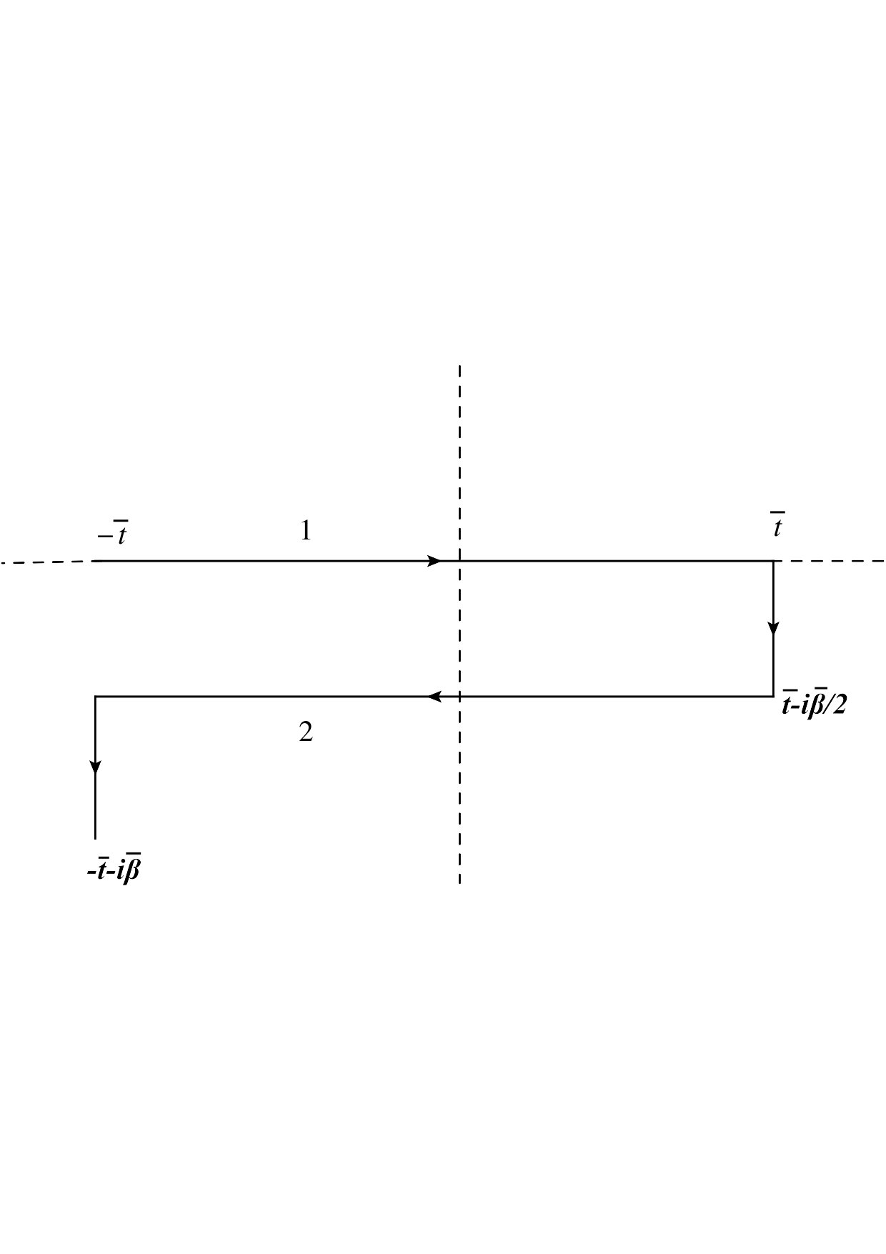 Figure 1
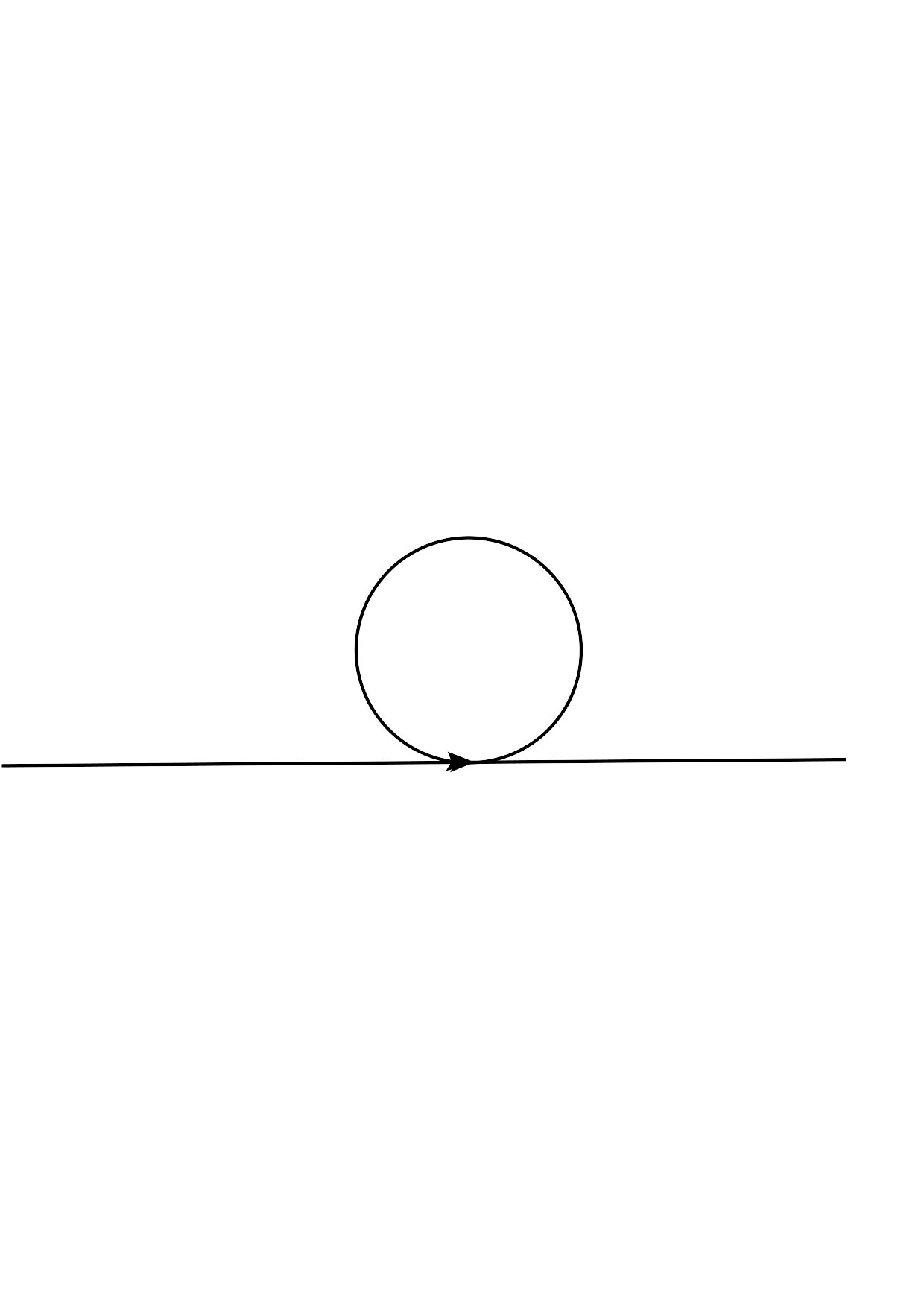 Figure 2
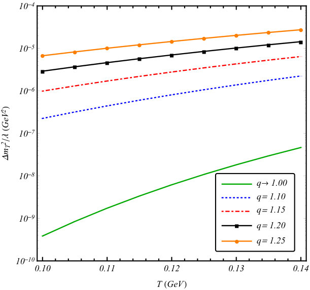 Figure 3
Peer Reviews
No public reviews on file for this paper yet. If you reviewed it on a platform where reviews are public (OpenReview, ICLR, NeurIPS, ICML), you can paste yours below so the community can read it here.
Videos
No videos yet. Explain this paper in a talk, walkthrough, or lecture? Add one.
Taxonomy
TopicsStatistical Mechanics and Entropy · Advanced Thermodynamics and Statistical Mechanics · Complex Systems and Time Series Analysis
ub
aainstitutetext: Variable Energy Cyclotron Centre, 1/AF, Bidhan Nagar, Kolkata - 700064, India bbinstitutetext: Homi Bhabha National Institute, Anushaktinagar, Mumbai, India ccinstitutetext: Bogoliubov Laboratory of Theoretical Physics, Joint Institute for Nuclear Reseach, Dubna, Russia
Thermal Field Theory of the Tsallis statistics
Mahfuzur Rahaman c
Trambak Bhattacharyya a,b
Jan-e Alam
Abstract
Classical and quantum Tsallis distributions have been widely used in many branches of natural and social sciences. But, the quantum field theory of the Tsallis distributions is relatively a less explored arena. In this article, we derive the expression for the thermal two-point functions for the Tsallis statistics with the help of the corresponding statistical mechanical formulations. We show that the quantum Tsallis distributions used in the literature appear in the thermal part of the propagator much in the same way the Boltzmann-Gibbs distributions appear in the conventional thermal field theory. As an application of our findings, we calculate the thermal mass in the scalar field theory within the realm of the Tsallis statistics.
1 Introduction
In spite of a remarkable success of the Boltzmann-Gibbs (BG) statistical mechanics, there exist many systems which may not be describable by this formulation tsallisbook ; tsallisgellmann . Some generalized concepts are needed to deal with such systems. These systems often contain fluctuations (of temperature, number density etc.) inside their boundary, and/or they may experience long-range correlation. It has been established wilk ; wilkprc ; wilkchaos ; biroprl that these kinds of systems may be understood from a generalization of the Boltzmann-Gibbs formulations developed by C. Tsallis tsallis88 , and is known as the ‘Tsallis statistics’.
Since then, the Tsallis-like single particle distributions have been used in many branches of natural plastinopla ; olbert ; tsalliscosmic ; beckcosmic ; rafelskidiffu ; tbsmdiffu ; chem ; compu ; bio ; bhupalastro and social sciences eco ; cogni ; lingu , and the field of high energy collisions is no exception PHENIX1 ; CMS1 ; CMS2 ; ALICE_deuteron ; Biro09 ; Cleymans09 ; Cleymans12 ; Cleymans13 ; khandai ; TsallisTaylor ; tsallisraa ; Grigoryan17 ; lacey ; ishihara ; bcmmp ; bcmpst ; Azmi14 ; deppmanYMTsFract1 ; deppmanYMTsFract2 . These studies have now established that the a global observable like the hadronic transverse momentum distribution generated from the high energy collisions (of protons on protons, for example) is describable by the ‘Tsallis-like’ distributions up to a very high range of transverse momentum () Azmi14 . Of particular importance is the power-law phenomenological distribution function below Cleymans12 ; bcmmp ,
[TABLE]
where is a constant factor, is the single particle energy, and is rapidity. Many of the above-mentioned articles utilize this distribution to describe the experimental data. The distribution in eq. (1) is popularly known as the ‘Tsallis distribution’ which is described by the entropic parameter and the Tsallis (inverse) temperature . It has been established in ref. wilk that in a system of fluctuating temperature zones, is the average inverse temperature and is related to the relative variance in temperature. In the limit , eq. (1) becomes Boltzmann like,
[TABLE]
and according to ref. wilk , this implies a gradual disappearance of fluctuations inside the system.
There have been attempts to verify whether the phenomenological Tsallis distribution belongs to the exact Tsallis statistical mechanical formulations. Recently, it has been shown in Parvan19 that the transverse momentum spectra obtained from the exact Tsallis statistical mechanics is expressible in terms of a series expansion, and the zeroth order approximation of that series (for Maxwell-Boltzmann particles) is the distribution given by eq. (1).
In the present article, we are, however, interested in the quantum extensions of the Tsallis distribution. The forms of the quantum distributions we concentrate upon are given below Hasegawa ,
[TABLE]
Many other studies conroypla ; buyupla ; penpla ; millerpla ; millerprd ; Mitra18 use a slightly different form of the Tsallis quantum distributions given by,
[TABLE]
where positive(negative) sign appears for the fermions(bosons). While eqs. (3), and (4) can be obtained from the statistical mechanical formulations proposed by Tsallis Tsallis3 , eq. (5) fails to show this connection. We will show that as a quantum extension of eq. (1) our results are consistent with the expressions given in eqs. (3) and (4). It is worth observing that the Tsallis quantum distribution approaches the corresponding Boltzmann-Gibbs quantum distribution when tends to 1. Also, in the high temperature regime (), both of them approach the classical limit given by eq. (1).
It is well-known that the Boltzmann-Gibbs quantum distributions appear naturally through the two point functions evaluated using the techniques of the thermal quantum field theory (see e.g. bellac ; das ; kapusta ; smallik ). In the present work, we calculate the thermal two-point functions from the Tsallis generalization of thermal field theory in which the Tsallis quantum distributions given by eqs. (3), and (4) appear. The generalization of thermal field theory in the Tsallis statistics has been addressed in ref. niegawa , which, however, adapts the Tsallis statistical mechanical formulation Tsallis3 that uses a definition of the expectation values different from that being used in the present paper (and in the phenomenological studies). Authors in ref. olemskoi also study the evolution of the most probable values of the order parameters by using the field theory of non-additive system. However, the mentioned articles do not attempt to provide an explicit derivation of the quantum distributions given in eqs. (3), and (4) which are of importance in the theoretical, phenomenological, and experimental studies. This is why in the present work we derive the quantum Tsallis distributions given by eqs. (3), and (4) using the generalized techniques of thermal field theory. It is expected that the present work will address the need of a quantum field theory of the Tsallis distributions used in various branches of physics and beyond.
The paper is organized as follows. In the next section the basic formulations of the Tsallis statistical mechanics are discussed. In sections 2, and 3 the real time thermal propagators for scalar and Dirac particles are derived respectively. The results obtained in section 2 have been applied to estimate the thermal mass of real scalar bosons in section 5. Section 6 is devoted to summary, discussions, and conclusions.
2 Free Tsallis thermal propagator for the real scalar field theory
2.1 Some basic formulae and relations
The Tsallis statistics begins with a generalized definition of entropy Tsallis3 which, if written in terms of density matrix , takes the following form,
[TABLE]
subject to the normalization condition,
[TABLE]
The thermal expectation value is given by Tsallis3 ; Abe ,
[TABLE]
approaches the Boltzmann-Gibbs-Shannon entropy given by when approaches 1.
By extrimizing the potential function (for chemical potential, ),
[TABLE]
for temperature with respect to density matrix, we get,
[TABLE]
is the Hamiltonian such that where is the energy of the system. Partition function is given by,
[TABLE]
The prime (′) in trace implies the Tsallis cut-off condition, which means that the trace is taken over the energy eigen values which satisfy the criterion \big{[}1+\beta(q-1)E\big{]}\geq 0. The Boltzmann-Gibbs density matrix can be obtained when . Given the Tsallis cut-off condition, we can write the density operator in terms of the -exponential operator defined as follows,
[TABLE]
The above equation implies,
[TABLE]
In the limit , the -exponential operator approaches the conventional exponential counterpart.
With the help of the generalized definition of the expectation values, the Tsallis thermal propagator for the real scalar field (with ) on a contour C can be defined as,
[TABLE]
where
[TABLE]
and
[TABLE]
are the advanced and the retarded propagators respectively. represents the time ordering operator and and are two arbitrary points on the contour C (Fig. 1).
To investigate the region in the complex time plane (see ref. Mills ) where and are defined, let us consider the advanced part of the thermal propagator.
By introducing the completeness relation, =, where defines the spectrum of , and by replacing the Heisenberg field by Schrodinger field as , we get,
[TABLE]
where we have used . The unbounded spectrum of determines the convergence of the sums and consequently choose the domain in which can be defined. The sum over and converge respectively for,
[TABLE]
and . Combining these two we get,
[TABLE]
In the limit , the above convergence condition becomes that of the Boltzmann-Gibbs statistics,
[TABLE]
In the case of Tsallis statistics, we have to consider a contour which always respects the convergence condition eq. (17). We can take the symmetrical contour suggested in Refs. Schwinger ; Keldysh ; Niemi ; Umezawa1 ; Umezawa2 shown in Fig. 1.
2.2 KMS relation in the Tsallis statistics
We derive below the Kubo-Martin-Schwinger (KMS) relation (Kubo ; Martin ) within the scope of Tsallis statistics. The KMS relation is the one connecting the retarded and the advanced parts of the propagator. Writing the explicit form of the retarded propagator we obtain the following equation,
[TABLE]
where
[TABLE]
and
[TABLE]
It can be observed from eq. (19) that the KMS relation acts as a boundary condition that imposes a periodicity in the propagator in terms of the time variable . It is also observed that the KMS relation of the Tsallis statistics is energy dependent biro . In the limit , eq. (19) reduces to its Boltzmann-Gibbs counterpart bellac ; das ,
[TABLE]
and the energy dependence do not appear. It is worthwhile to mention that the periodicity condition is exclusive to the bosonic particles. For the fermions, one encounters anti-periodicity in the time axis (see section 3).
The invariance of the two point functions under time translation stated as, can be ensured by the condition , where and are the Fourier transforms of and respectively. It may be noted here that in the limit , and consequently it becomes straightforward to show the time invariance of the two point functions.
2.3 Calculating Tsallis propagator using the differential equation method
After obtaining the KMS relation, we derive the thermal propagator for the real scalar particles by solving the corresponding field equation, i.e. we need to solve the following equation,
[TABLE]
We can take the following Fourier transform as the spatial coordinates are not associated with boundary conditions as opposed to the time coordinate:
[TABLE]
Putting eq. (24) in eq. (23) and using the integral representation of the space-dependent part of the Dirac-delta function, we obtain
[TABLE]
Comparing the r.h.s with the l.h.s we get,
[TABLE]
where is the single particle energy, and .
For , the solution of eq. (26) is a linear combination of and . We can write the retarded and the advanced part of the Green’s function (or propagator) as the linear combinations of these functions with coefficients depending on ,
[TABLE]
The unknown coefficients can be found with the help of the modified KMS relation in eq. (19) as one of the boundary conditions along with the following ones arfken ,
[TABLE]
Using the above boundary conditions in eq. (LABEL:23) we get
[TABLE]
and
[TABLE]
which when put into eq. (LABEL:23), yield,
[TABLE]
Using eqs. (LABEL:23) and (19), we get
[TABLE]
Now, is the total energy of the state ’ which is populated by many particles. If there are particles each with energy , then we may write
[TABLE]
Comparing the coefficients of and in both the sides of eq. (LABEL:30) we get,
[TABLE]
At this point, we introduce the following approximation for the power-law,
[TABLE]
If we write,
[TABLE]
, and can be written as,
[TABLE]
Using the values of and , we get and ,
[TABLE]
Hence, the thermal propagator can be written as,
[TABLE]
where the indices , and denote on which part (1 or 2) of the contour lies (see Fig. 1).
The components of the momentum space thermal propagator can be found by taking temporal Fourier transform
[TABLE]
Now, the above integration in eq. (43) can be performed by choosing two points on any one of the two horizontal line shown in Fig. 1. Propagators containing lying on the vertical lines vanish due to the Riemann-Lebesgue lemma Titchmarsh . We can take two points on two horizontal lines in four different ways,
- •
and both lie on line 1.
- •
and both lie on line 2.
- •
lies on line 1 and lies on line 2.
- •
lies on line 2 and lies on line 1 .
These four cases can be implemented through the following choices of theta functions in that order,
. 2. 2.
. 3. 3.
. 4. 4.
.
Let us now calculate the ‘11’ component of the real time thermal propagator which may be written as follows,
[TABLE]
where we have replaced by which is again replaced with in the second term involving . Now, the integrands are oscillatory and they diverge at . To avoid this divergence while carrying out the integral, we have added an infinitesimally small imaginary part in which will be made to vanish finally. After integrating, we obtain,
[TABLE]
We simplify the above equation further by using the Sokhotski-Plemelj formula plemeljform ,
[TABLE]
where ‘’ denotes the principal value, to obtain,
[TABLE]
where , for invariant mass . In the limit , we get back the real time BG bosonic propagator,
[TABLE]
If we compare with the BG thermal field theoretic results in eq. (48), the coefficient of the quantity in eq. (47) can be identified to be the Tsallis Bose-Einstein distribution given by,
[TABLE]
where
[TABLE]
It can easily be checked that in the limit, one gets . It is interesting to note that in this limit the TB statistics goes to GB statistics as a consequence it becomes simple to prove the invariance of two point functions under time translation. The form of this distribution is identical with the result obtained in Hasegawa . This result may also be obtained from the factorization approximation of the zeroth term approximation of the result obtained in Parvan19 . The above two references calculate the Tsallis Bose-Einstein distribution from Tsallis statistical mechanical formulations, and hence the form of the distribution obtained in eq. (47) belongs to the Tsallis statistical mechanics.
Next we proceed to calculate the . In this case (see Fig. 1) and
[TABLE]
Substituting and using the integral representation of delta function
[TABLE]
and using the approximation eq. (36), we finally get,
[TABLE]
In the limit , we get back the usual Boltzmann-Gibbs propagator,
[TABLE]
where is the Boltzmann-Gibbs bosonic distribution. Similarly we get, and . Then the matrix propagator is given by,
[TABLE]
where is the zero temperature term in the propagator. Substituting in place of the propagator in eq. (55) can be put in a diagonal form,
[TABLE]
The diagonalizing matrix is given by,
[TABLE]
Now, for free propagator
[TABLE]
which implies,
[TABLE]
Comparing the real and the imaginary parts from both the sides we obtain,
[TABLE]
where the sign function is used to carry out the following transformation,
[TABLE]
3 Free Tsallis thermal propagator for the fermions
The Dirac thermal propagator in the Tsallis statistics may be defined by,
[TABLE]
where , is the partition function for vanishing chemical potential. The Dirac thermal propagator can be written as,
[TABLE]
where
[TABLE]
Next, we quote the KMS relation for the Dirac field. The derivation is similar to that for the bosons.
[TABLE]
where is given by eq. (20). In the limit , the equation reduces to its Boltzmann-Gibbs counterpart,
[TABLE]
Calculations in the scalar case and in the Dirac case closely follow each other if we write the fermion propagator in terms of the scalar propagator in the following manner,
[TABLE]
Spatial Fourier transform of yields,
[TABLE]
With the help of eqs. (69), and (70) we obtain,
[TABLE]
The advances and retarded parts are given by,
[TABLE]
Guided by eqs. (LABEL:23), (32) from the scalar case and by taking the spatial Fourier transform of the eq. (67) we obtain the following equation,
[TABLE]
where and . Equating the coefficients of , and employing the approximation indicated in eq. (36) we get,
[TABLE]
Identifying
[TABLE]
which is the single particle distribution for the Tsallis fermions, we can write , and as,
[TABLE]
So, the fermion thermal propagator can be written as,
[TABLE]
Taking temporal Fourier transform, and invoking the time translational invariance,
[TABLE]
where, as usual, represent points on the lines on the contour .
The computation of the components of yields,
[TABLE]
where . Also, we use the identity , replace , and utilize the integral representation of the Dirac-delta function. Comparing the expression of in eq. (81) with the BG field theoretic results, we can identify given in eq. (76) as the Tsallis distribution for the Dirac particles. Next we compute ,
[TABLE]
Let us define two quantities
[TABLE]
and
[TABLE]
Using which, we can write,
[TABLE]
Similarly we can get and . Hence, the matrix representing the real time propagator is given by,
[TABLE]
Using and , the above matrix can be written as,
[TABLE]
The above expression can be put in a diagonal form as follows,
[TABLE]
where the diagonalizing matrix is given by,
[TABLE]
We find out the relationship between the ‘11’ component of the free fermion propagator, and the free propagator(diagonalized) in a way similar to what has been done for the bosonic fields in eq. (LABEL:relation). We simply quote the results below,
[TABLE]
4 Diagonalization
In the above calculations, we observe that the real time thermal propagators are having matrix structure which corresponds to a doubling of degrees of freedom. This doubling of degrees of freedom in the real time thermal field theory can be handled by considering the diagonal form of the propagators given by eqs. (56) and (88). In order to do so, we can start from the matrix form of the Dyson-Schwinger equation. The Dyson-Schwinger equation connects the interacting and the free thermal propagators through the self-energy matrix. Denoting the bosonic free propagator, interacting propagator and the self-energy matrices (denoted by bold-faced letters) as , , and respectively, the corresponding Dyson-Schwinger equation is given by,
[TABLE]
The matrix , given by eq. (57), diagonalizes the free propagator , the interacting propagator and the self-energy , so that the self-energy is of the form,
[TABLE]
which, in turn, diagonalizes (denoted by ’bar’) eq. (91) and reduces the matrix equation to an ordinary equation,
[TABLE]
having the solution
[TABLE]
where is the complete diagonalized thermal propagator and the is the diagonalized self-energy function. It is evident from eq. (92) that,
[TABLE]
Also, the diagonalized self-energy can be obtained entirely from any one component, say , from eq. (92) as,
[TABLE]
In a similar way, for the Dirac propagators, the Dyson-Schwinger equation reads,
[TABLE]
The matrix given by eq. (89), which diagonalizes the free propagator , also diagonalizes the full propagator and the self-energy . Then the form of is,
[TABLE]
which reduces the matrix equation (97) to an ordinary equation,
[TABLE]
with the solution
[TABLE]
It is evident from eq. (98) that,
[TABLE]
The diagonalized self-energy can be obtained entirely from any one component, say , from eq. (98) as,
[TABLE]
5 Application: thermal mass of the scalar particles
In this section we will compute the thermal mass of the scalar particles as an application of the thermal field theory formalism developed so far for the Tsallis statistics. Thermal mass is given by the real part of self-energy, which we calculate using the ‘11’ component of the Tsallis thermal propagator. We calculate the thermal mass in the self-interacting theory for which the Lagrangian density is given by,
[TABLE]
The leading order mass shift due to thermal effects , which involves the diagram shown in Fig. 2, can be obtained as das ,
[TABLE]
where . The infinite sum converges for . This condition is satisfied because in this work we take and consider massive particles. We use the following Mellin-Barnes representation (for details see BhattaCleMog ; smirnov ) in the last line of the above equation,
[TABLE]
for , and , where and , and obtain,
[TABLE]
The above expression has poles at the positive and negative values given by due to the appearance of the gamma functions in the numerator. We wrap the contour clockwise to include the poles at . While doing so, the condition guarantees the convergence of the integral at . Summing up the residues due to the poles at , we obtain the following expression in terms of the summation of an infinite series whose terms contain the hypergeometric functions arfken ,
[TABLE]
Though the series appears to contain an infinite number of terms, we have verified that for the , , and mass values used in Fig. 3, the terms in the series die down very fast with increasing . So, we may choose an upper cut-off (convergence is obtained here for here) and obtain the following expression for the thermal mass in the theory within the scope of the Tsallis statistics,
[TABLE]
For , the above integral approaches the Boltzmann-Gibbs result das ; kapusta ,
[TABLE]
The variation of the quantity given by eq. (108) with is depicted in Fig.3. It is clear from the results displayed that in case of the Tsallis statistics, the magnitude of thermal mass is larger than that in the Boltzmann-Gibbs (BG) statistics. As expected, in the limit , the two results tend to merge with each other. It is important to mention at this point that in a small system like quark gluon plasma (QGP), where applications of the BG statistics is uncertain, the thermal field theoretic formulation developed in this work for the Tsallis statistics will have crucial importance. The thermal spectral functions of the quarks and gluons kyagi estimated using the BG and Tsallis statistics will differ (as is the case for interaction) which may have significant impact on the signals of QGP cywong .
6 Summary and conclusions
In this work we have derived the real time thermal propagators for scalar and Dirac fields within the scope of the Tsallis statistics and calculated the thermal mass of a scalar particle subjected to interaction using the generalized thermal two-point function. It has been observed that the quantum Tsallis distributions given by eqs. (3), and (4) appear in the thermal part of the Tsallis two-point functions. We also observe that when the entropic parameter approaches 1, the classical and quantum Boltzmann-Gibbs thermal propagators are recovered. In the calculations of the thermal mass we observe a significant increase in the scaled mass shift which approaches the Boltzmann-Gibbs limit as approaches
- Hence, the present work may be seen as a stepping stone towards the generalization of the Boltzmann-Gibbs finite temperature quantum field theory developed with the aid of the Tsallis statistical mechanical formulations. As indicated, this formalism and its extension may help one to compute the quantities like thermal mass, decay rate, energy loss in more realistic situations dealing with fluctuating ambience, and/or long-range correlations.
However, the calculation uses an approximation given by eq. (36) which may limit its applicability, and in turn, that of the distributions given by eqs. (1), (3), and (4). As already mentioned in the introduction, these distributions are the approximate forms of the Tsallis single particle distributions, and a more general formula for the propagators is required. In this article, we, however, were interested in the approximate forms of the distributions, and their connection with a thermal quantum field theory. The connection between the most general form of the Tsallis single particle distribution Parvan19 and a thermal quantum field theory will be a subject matter of our next work. In addition to that, the definition of the expectation values is according to the choice made in deriving the Tsallis distributions in eqs. (1), (3), and (4). A more consistent definition of the expectation values needs to be incorporated in future, too.
Acknowledgements.
M.R. would like to thank the Department of Atomic Energy, Govt. of India for financial support. T.B. thanks Bogoliubov Laboratory of Theoretical Physics, JINR for the travel grant to visit Variable Energy Cyclotron Centre (VECC), Kolkata, India where this work began. He also thanks VECC for the support extended to him during his visit. The authors thank Dr. Alexandru Parvan for very fruitful discussions.
The reference list from the paper itself. Each links out to its DOI / PubMed record.
- 1(1) C Tsallis, Introduction to non extensive statistical mechanics , Springer Science+Business Media (2009).
- 2(2) Murray Gell-Mann, and Constantino Tsallis (eds.), Nonextensive Entropy – Interdisciplinary Applications , Oxford University Press (2003)
- 3(3) G. Wilk, and Z. Włodarczyk, Interpretation of the Nonextensivity Parameter q 𝑞 q in Some Applications of Tsallis Statistics and Lévy Distributions, Phys. Rev. Lett. 84 (2000) 2770.
- 4(4) G. Wilk, and Z. Włodarczyk, Multiplicity fluctuations due to the temperature fluctuations in high-energy nuclear collisions, Phys. Rev. C 79 (2009) 054903.
- 5(5) G. Wilk, and Z. Włodarczyk, The imprints of nonextensive statistical mechanics in high-energy collisions, Chaos Solitons Fractals 13 (2001) 581.
- 6(6) T.S. Biró, and A. Jakovác, Power-law tails from multiplicative noise, Phys. Rev. Lett. 94 (2005) 132302.
- 7(7) C Tsallis, Possible generalization of Boltzmann-Gibbs statistics, J. Stat. Phys. 52 (1988) 479.
- 8(8) A.R. Plastino, and A. Plastino, Stellar polytropes and Tsallis’ entropy, Phys. Lett. A 174 (1993) 384.