An analysis of binary microlensing event OGLE-2015-BLG-0060
Y. Tsapras, A. Cassan, C. Ranc, E. Bachelet, R. Street, A. Udalski, M., Hundertmark, V. Bozza, J. P. Beaulieu, J. B. Marquette, E. Euteneuer, The, RoboNet team: D. M. Bramich, M. Dominik, R. Figuera Jaimes, K. Horne, S. Mao,, J. Menzies, R. Schmidt, C. Snodgrass, I. A. Steele

TL;DR
This paper thoroughly analyzes a binary microlensing event using extensive multi-telescope data, successfully constraining the physical parameters of the lens system and demonstrating the importance of follow-up observations for detailed event characterization.
Contribution
First comprehensive coverage of an anomalous microlensing event enabling precise physical parameter estimation of the lens system.
Findings
Lens system consists of two stars with masses ~0.87 and 0.77 solar masses.
Distance to the lensing system is approximately 6.41 kpc.
Projected separation between the binary components is about 13.85 AU.
Abstract
We present the analysis of stellar binary microlensing event OGLE-2015-BLG-0060 based on observations obtained from 13 different telescopes. Intensive coverage of the anomalous parts of the light curve was achieved by automated follow-up observations from the robotic telescopes of the Las Cumbres Observatory. We show that, for the first time, all main features of an anomalous microlensing event are well covered by follow-up data, allowing us to estimate the physical parameters of the lens. The strong detection of second-order effects in the event light curve necessitates the inclusion of longer-baseline survey data in order to constrain the parallax vector. We find that the event was most likely caused by a stellar binary-lens with masses and . The distance to the lensing system is 6.41 kpc and the…
Click any figure to enlarge with its caption.
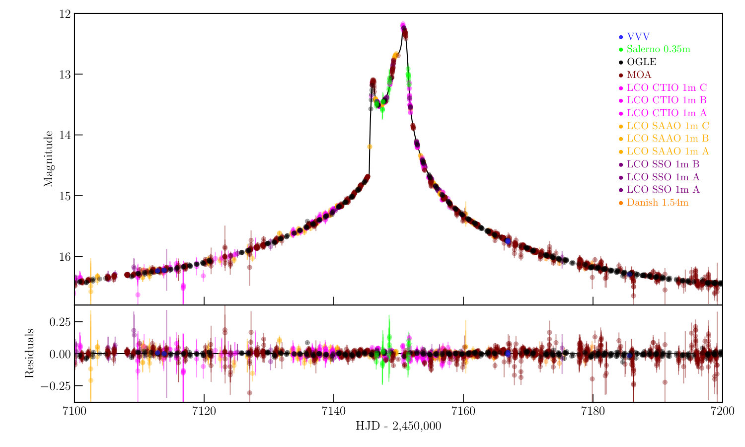 Figure 1
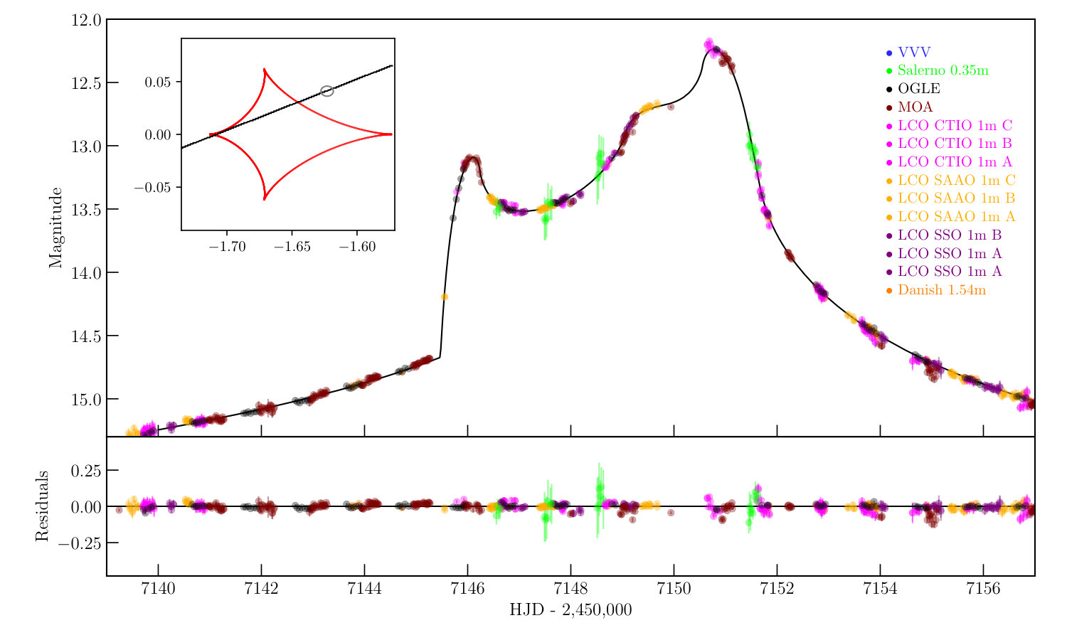 Figure 3
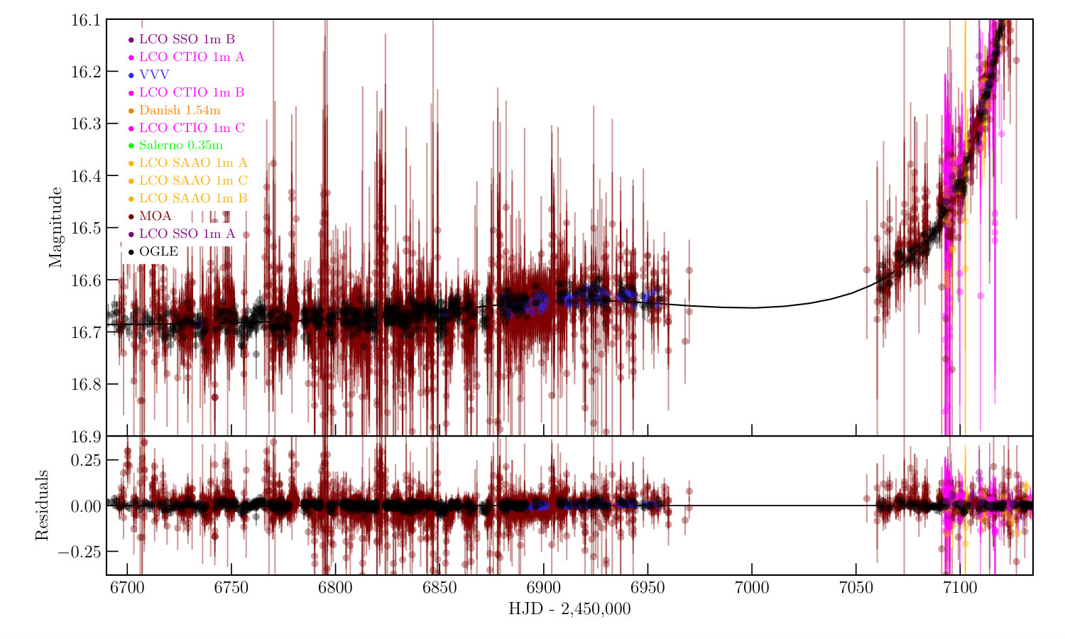 Figure 3
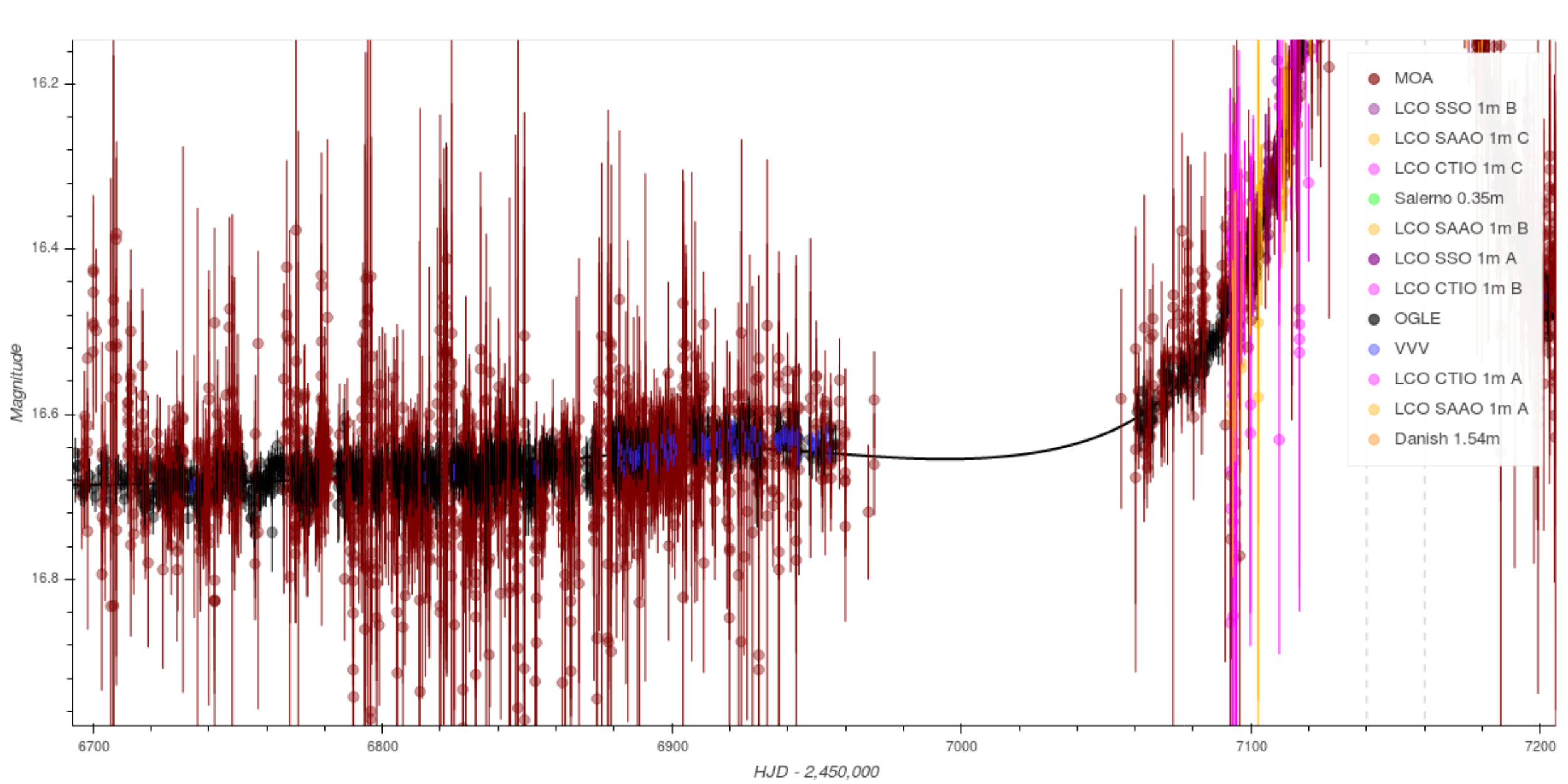 Figure 4
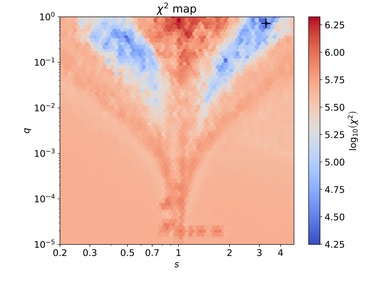 Figure 5
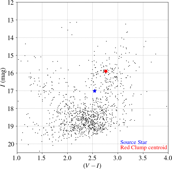 Figure 6
| Group | Telescope | Passband | Data points |
| OGLE | 1.3m Warsaw Telescope, Las Campanas, Chile | 1629,101 | |
| MOA | 1.8m MOA Telescope, Mount John, New Zealand | 5674,71 | |
| RoboNet | 1.0m LCO (Dome A), CTIO, Chile | SDSS-i’ | 176 |
| RoboNet | 1.0m LCO (Dome B), CTIO, Chile | SDSS-i’ | 83 |
| RoboNet | 1.0m LCO (Dome C), CTIO, Chile | SDSS-i’ | 138 |
| RoboNet | 1.0m LCO (Dome A), SAAO, South Africa | SDSS-i’ | 92 |
| RoboNet | 1.0m LCO (Dome B), SAAO, South Africa | SDSS-i’ | 60 |
| RoboNet | 1.0m LCO (Dome C), SAAO, South Africa | SDSS-i’ | 86 |
| RoboNet | 1.0m LCO (Dome A), SSO, Australia | SDSS-i’ | 65 |
| RoboNet | 1.0m LCO (Dome B), SSO, Australia | SDSS-i’ | 62 |
| MiNDSTEp | 1.5m Danish Telescope, La Silla, Chile | LIred | 85 |
| MiNDSTEp | 0.6m Salerno Telescope, Salerno, Italy | 25 | |
| VVV | 4.1m VISTA Telescope, Paranal, Chile | 240 | |
| Note: For a description of the MiNDSTEp LIred bandpass see Skottfelt et al. (2015). | |||
| For a description of the MOA bandpasses see Sako et al. (2008). | |||
| Parameter | static (npar=7) | parallax (npar=9) | parallax+orbital motion (npar=11) | ||
|---|---|---|---|---|---|
| 7738.59 | 7589.02 | 7571.63 | 7383.51 | 7390.10 | |
| (HJD’) | 7030.72 0.75 | 7038.65 0.69 | 7039.06 0.70 | 7046.22 0.88 | 7046.07 0.88 |
| 0.779 0.004 | 0.747 0.003 | -0.746 0.003 | 0.878 0.013 | -0.831 0.011 | |
| (days) | 73.90 0.18 | 72.93 0.18 | 72.81 0.18 | 68.19 0.55 | 66.703 0.559 |
| 3.487 0.005 | 3.433 0.005 | 3.430 0.005 | 3.459 0.006 | 3.470 0.009 | |
| 0.817 0.006 | 0.884 0.006 | 0.885 0.006 | 0.837 0.007 | 0.834 0.009 | |
| (radians) | 2.6952 0.0006 | 2.6900 0.0007 | -2.6894 0.0007 | 2.622 0.008 | -2.655 0.007 |
| 0.0046 | 0.0048 | 0.0047 | 0.0047 | 0.0047 | |
| – | 0.013 0.002 | -0.018 0.002 | 0.130 0.012 | -0.087 0.010 | |
| – | -0.046 0.003 | -0.044 0.003 | -0.045 0.005 | -0.064 0.004 | |
| (yr-1) | – | – | – | 0.26 0.09 | 0.63 0.09 |
| (yr-1) | – | – | – | -0.28 0.02 | 0.22 0.02 |
| Parameter | OGLE + MOA | OGLE | follow-up |
|---|---|---|---|
| /dof | 0.878 | 0.883 | 0.779 |
| (HJD’) | 7037.92 0.76 | 7048.54 1.31 | 7045.13 0.95 |
| -0.756 0.004 | -0.709 0.008 | -0.720 0.006 | |
| (days) | 72.98 0.19 | 70.28 0.31 | 68.98 0.30 |
| s | 3.433 0.006 | 3.353 0.010 | 3.374 0.008 |
| q | 0.870 0.007 | 0.939 0.012 | 0.867 0.011 |
| (radians) | -2.687 0.001 | -2.689 0.002 | -2.703 0.002 |
| 0.0048 | 0.0051 | 0.0050 | |
| -0.004 0.004 | -0.022 0.004 | -0.003 0.003 | |
| -0.049 0.003 | -0.055 0.005 | -0.057 0.006 | |
| (yr-1) | – | – | – |
| (yr-1) | – | – | – |
| Parameter | Value |
|---|---|
| Mass of lens star #1 () | 0.87 0.12 |
| Mass of lens star #2 () | 0.77 0.11 |
| Distance to the lens () | 6.41 0.14 kpc |
| Projected star-star separation () | 13.85 0.16 AU |
| Einstein radius () | 0.62 0.08 mas |
| Geocentric proper motion () | 3.16 0.39 mas yr-1 |
Peer Reviews
No public reviews on file for this paper yet. If you reviewed it on a platform where reviews are public (OpenReview, ICLR, NeurIPS, ICML), you can paste yours below so the community can read it here.
Videos
No videos yet. Explain this paper in a talk, walkthrough, or lecture? Add one.
An analysis of binary microlensing event OGLE-2015-BLG-0060
Y. Tsapras1 A. Cassan2, C. RancM3, E. Bachelet3, R. Street3, A. UdalskiO1, M. Hundertmark1, V. BozzaR10,S2, J. P. Beaulieu2,4, J. B Marquette2, E. Euteneuer1, The RoboNet team: D. M. BramichR18, M. DominikR3, R. Figuera JaimesR3,R16, K. HorneR3, S. MaoR16,R15,R17, J. MenziesR8 R. Schmidt1, C. SnodgrassR13,R19, I. A. SteeleR4, J. Wambsganss1,R20 The OGLE collaboration: P. MrózO1, M.K. SzymańskiO1, I. SoszyńskiO1, J. SkowronO1, P. PietrukowiczO1 S. KozłowskiO1, R. PoleskiO2, K. UlaczykO1, M. PawlakO1 The MiNDSTEp collaboration: U. G. JørgensenP1, J. SkottfeltP23,P1, A. PopovasP1, S. CiceriP10, H. KorhonenP21,P11,P1, M. KuffmeierP1, D. F. EvansP14, N. PeixinhoP15,P27, T. C. HinseP16, M. J. BurgdorfP17, J. SouthworthP14, R. TronsgaardP18, E. KerinsR17, M.I. AndersenP21, S. RahvarP22, Y. WangP24, O. WertzP25, M. RabusP26,P10, S. Calchi NovatiS3, G. D’AgoS4,R10, G. ScarpettaS5,R10, L. ManciniP28,P29,P30 The MOA collaboration: F. AbeM2, Y. AsakuraM2, D. P. BennettM3,M12, A. BhattacharyaM3,M12, M. DonachieM4, P. EvansM4, A. FukuiM5, Y. HiraoM1, Y. ItowM2, K. KawasakiM1, N. KoshimotoM1, M.C.A. LiM4, C.H. LingM6, K. MasudaM2, Y. MatsubaraM2, Y. MurakiM2, S. MiyazakiM1, M. NagakaneM1, K. OhnishiM7, N. RattenburyM4, To. SaitoM8, A. SharanM4, H. ShibaiM1, D.J. SullivanM9, T. SumiM1, D. SuzukiM3, P.J. TristramM10, T. YamadaM11, A. YoneharaM11
*Affiliations appear at the end of the paper
E-mail: [email protected]
(Published in MNRAS 30 May 2019. https://doi.org/10.1093/mnras/stz1404)
Abstract
We present the analysis of stellar binary microlensing event OGLE-2015-BLG-0060 based on observations obtained from 13 different telescopes. Intensive coverage of the anomalous parts of the light curve was achieved by automated follow-up observations from the robotic telescopes of the Las Cumbres Observatory. We show that, for the first time, all main features of an anomalous microlensing event are well covered by follow-up data, allowing us to estimate the physical parameters of the lens. The strong detection of second-order effects in the event light curve necessitates the inclusion of longer-baseline survey data in order to constrain the parallax vector. We find that the event was most likely caused by a stellar binary-lens with masses and . The distance to the lensing system is 6.41 kpc and the projected separation between the two components is 13.85 AU. Alternative interpretations are also considered.
keywords:
gravitational lensing: micro, methods: observational, techniques: photometric, Galaxy: bulge
††pubyear: 2019††pagerange: An analysis of binary microlensing event OGLE-2015-BLG-0060–A
1 Introduction
There are two unique aspects to gravitational microlensing that set it apart from other exoplanet detection methods. Firstly, it is most sensitive to planets at separations 1-10AU from their hosts (Tsapras et al., 2016; Suzuki et al., 2016; Cassan et al., 2012; Tsapras et al., 2003), a region of great relevance to planetary formation theories (Ida et al., 2013), as this typically places the planet beyond the snow-line111The snow-line is the distance from a proto-star beyond which any water present in the proto-planetary disk will be in the form of ice grains. of the host star (Armitage et al., 2016), a region largely inaccessible to the transit and radial-velocity methods. Secondly, it detects planets around faint stars at distances of several thousand parsec (Penny et al., 2016), whereas almost every planet discovered to date by other methods lies only within a few hundred parsec from the Sun. Since stellar metallicity decreases with distance from the centre of the Galaxy (Ivezić et al., 2008), microlensing planets may have formed in more metal-rich environments leading to a potentially different statistical distribution compared to the sample of nearby planets. This hypothesis can only be explored through microlensing.
The phenomenon of gravitational microlensing occurs when a foreground star gravitationally lenses a luminous background star, causing its brightness to gradually increase, and then gradually decrease, over a period of several days to months (Paczynski, 1986). The angular distance between the images generated by the lensing event is generally too small to resolve with current technology so that only the change in brightness of the background object, commonly referred to as the source star, is observed. The only known exception to date is the nearby microlensing event TCP J0507+2447, detected on October 25th 2017 by Japanese amateur astronomer Tadashi Kojima, for which Dong et al. (2019) managed to resolve, for the first time, the two microlensing images using the GRAVITY interferometer on the Very Large Telescope (VLT). A few very bright microlensing events per year might also be within the reach of the PIONIER instrument (Cassan & Ranc, 2016).
Should the foreground lensing object be a star-star or star-planet system, its exact geometric alignment and physical parameters may leave an imprint on an otherwise symmetric light curve (Dominik, 2010; Gaudi, 2012; Tsapras, 2018). These anomalous features can be detected and sampled with frequent (hourly to daily) observations, depending on the particular event. Due to the transient and unpredictable nature of microlensing events, it is often not possible to distinguish between planetary and stellar binary anomalies when they are first identified. Follow-up observations are therefore typically executed for almost all events where there is evidence of ongoing anomalies and the light curves are continuously re-assessed through real-time modeling. A full characterisation is usually obtained only after the event has expired and returned to its baseline brightness.
Recent results from microlensing campaigns suggest that ice and gas giant planets are a relatively common feature (35%) around K and M-dwarf stars (Gould et al., 2010). Microlensing searches have also identified a number of very massive cool planets (Batista et al., 2011; Tsapras et al., 2014; Koshimoto et al., 2014; Skowron et al., 2015) and brown dwarf companions around low-mass stars (Street et al., 2013; Ranc et al., 2015; Han et al., 2016a), as well as several terrestrial to sub-Neptune mass planets (Beaulieu et al., 2006; Kubas et al., 2012; Gould et al., 2014; Shvartzvald et al., 2017), systems with multiple planets (Gaudi et al., 2008; Han et al., 2013) and the first possible detection of an exomoon (Bennett et al., 2014).
In this paper we present the analysis of binary microlensing event OGLE-2015-BLG-0060 using observations collected from 13 different telescopes spread out around the world, providing continuous monitoring of the event. Stellar binary microlensing events are discovered far more often than planetary ones and their diverse morphologies have been the subject of several past studies (Shin et al., 2017; Han et al., 2016b; Shin et al., 2012; Jaroszyński et al., 2010; Skowron et al., 2007). Typically, their caustic-crossing features are predicted well in advance, given differences in the smoothly rising part of the light curve as compared to single-lens events. OGLE-2015-BLG-0060 is of particular interest because it is the first time automated follow-up observations have achieved excellent coverage of all anomalous features without human involvement, demonstrating the potential of fully robotic observations in characterising microlensing events.
In Section 2 we provide a summary of the observations and data analysis. Section 3 describes the steps taken to model the event light curve and Section 4 the method used to determine the physical properties of the system. Finally, we provide a summary and conclusions in Section 5.
2 Observations and photometry
2.1 Survey and follow-up observations
Microlensing event OGLE-2015-BLG-0060 was announced on 2015 February 17 by the Early Warning System (EWS)222http://ogle.astrouw.edu.pl/ogle4/ews/ews.html of the Optical Gravitational Lensing Experiment (OGLE) survey (Udalski, 2003; Udalski et al., 2015) at equatorial coordinates , (J2000) (). OGLE observations were carried out with the 1.3-m Warsaw telescope at Las Campanas Observatory in Chile, with the 32-chip mosaic CCD camera. The event occurred in OGLE bulge field 504, which was imaged several times per night when not interrupted by weather or the full Moon, providing good coverage of the light curve when the bulge was visible from Chile. The OGLE survey reported a baseline -band magnitude for the blended star of 16.683, which was later revised to 16.933. The predicted maximum magnification at the time of announcement was very low, therefore the target was originally considered low priority for follow-up observations. The event was also independently picked up by the MOA survey (Sumi et al., 2003), using the 1.8-m MOA survey telescope at Mount John observatory in New Zealand, on 2015 March 17, and designated MOA-2015-BLG-071.
By mid-March 2015 it became apparent that it might be a high magnification event and the RoboNet (Tsapras et al., 2009) and MiNDSTEp (Dominik et al., 2010) teams began to observe it automatically. RoboNet observations were carried out using the southern ring of 1m robotic telescopes of the Las Cumbres Observatory (LCO) (Brown et al., 2013), a total of 8 telescopes located at the Cerro Tololo International Observatory (CTIO) in Chile, South African Astronomical Observatory (SAAO) in South Africa and Siding Spring Observatory (SSO) in Australia, providing continuous coverage of the event light curve. MiNDSTEp observations were carried out on the Danish 1.54m telescope at ESO La Silla in Chile and the 0.6m telescope at Salerno Observatory in Italy. New photometric reductions of VVV survey observations (Minniti et al., 2010) in the K-band at the location of the target were also included in the analysis, although none were obtained during the peak of the event.
The event was also observed by the Korea Microlensing Telescopes Network (KMTNet) (Kim et al., 2016), and their data are analysed separately. The Spitzer satellite also obtained observations of this target from June 12 (HJD2457186) to July 19 (HJD2457223), as part of an effort to constrain the parallax (Yee et al., 2015), but unlike the case of OGLE-2015-BLG-0966 (Street et al., 2016), these only cover the part of the light curve when the event is returning to baseline and provide no additional constraints. The Spitzer data are therefore not included in the final model the event.
The full light curve of OGLE-2015-BLG-0060 is shown in Figure 1, together with the best-fit model (cf. Section 3).
2.2 Detection of the anomaly
The first evidence that the event deviated from the standard single-lens Paczyński curve appeared on March 11, when the SIGNALMEN anomaly detector (Dominik et al., 2007) triggered an alert on the ARTEMiS event monitoring system (Dominik et al., 2008). The alert was propagated to the real-time modelling software RTModel (Bozza, 2010) to generate the first set of models, and complementary observation requests aimed at characterising the anomalous feature were automatically submitted to the LCO robotic telescopes (Hundertmark et al., 2018). On the same day, an email by V. Bozza alerted the community that the broad peak observed at the end of the 2014 season (HJD2456920, see Figure 5 in the Appendix) and the subsequent rise during 2015 (HJD2457080) were incompatible with a single lens, and that binary and planetary solutions were possible333The small deviation that triggered the follow-up observations was generated by the source approaching the first set of caustics at a distance of Einstein radii and took place well before the crossing of the second set of caustics.. A second report by Bozza on April 20, using updated data, predicted a possible caustic crossing. On May 3 (HJD2457145.5), strong deviations indicating a caustic crossing were detected in the RoboNet and then the OGLE and MiNDSTEp data. Shortly thereafter, D. Bennett alerted the community that a strong anomaly was ongoing, and V. Bozza pointed out that higher-order effects needed to be taken into account during the model fitting process. By May 9 (HJD2457151.5), V. Bozza had determined that the lens was likely to be a stellar binary, and on May 19 (HJD2457161.5) the Chungbuk National University group (CBNU, C. Han), using private KMTNet data that covered the anomalous feature, gave a preliminary estimate of the parameters of the system while the event was still ongoing. This solution was confirmed independently by V. Bozza on the same day.
2.3 Data reduction
The data used for the analysis presented in this paper and the telescopes used for the observations are listed in Table 1. Most observations were obtained in the band (SDSS-i′), while some images obtained by OGLE in were also used to generate a colour-magnitude diagram and classify the source star. MOA observations were performed with the MOA wide-band red filter, which is specific to that survey. We note that there are also observations obtained privately by the KMTNet survey, which will be analysed in a separate paper.
The photometric analysis of crowded-field observations is a challenging task. Images of the Galactic bulge contain thousands of stars whose point-spread functions (PSFs) often overlap, therefore aperture and PSF-fitting photometry offer very limited sensitivity to photometric deviations generated by the presence of low-mass planetary companions. For this reason, observers of microlensing events routinely perform difference image analysis (DIA) (Alard & Lupton, 1998), which offers superior photometric sensitivity under such conditions. For a given telescope and camera, the technique of difference image analysis uses a reference image444This can be either a single image or a combination of images taken under the best seeing conditions to which background, astrometric, photometric and point-spread-function corrections are applied to match the images of that same field taken at each individual epoch. The fitted model based on the reference image is then subtracted from the matching images to produce residual (or difference images). Stars that did not vary in brightness between the times the images were obtained leave no systematic residuals on the difference images, but stars that underwent brightness variations leave clear positive or negative residuals.
Most microlensing teams have developed custom DIA pipelines to reduce their observations. OGLE and MOA images were reduced using the photometric pipelines described in Udalski (2003) and Bond et al. (2001) respectively. RoboNet and MiNDSTEp observations were processed using customised versions of the DanDIA pipeline (Bramich et al., 2013; Bramich, 2008). Salerno data were reduced with a locally developed PSF-fitting pipeline. The data sets presented in this paper have been reprocessed to optimise photometric precision and it is these data we used as input when modelling the microlensing event. They are available for download from the online version of the paper.
3 Modelling
3.1 Wide exploration of the parameter space
The general shape of the OGLE-2015-BLG-0060 light curve, shown in Figure 1, displays typical features associated with a binary-lens caustic-crossing event: a sharp rise in brightness as the source enters the caustic at HJD2457146 (3 May), then a drop in brightness as the source traverses the interior of the caustic structure, followed by another sharp rise in brightness as the source exits the caustic at HJD2457150 (7 May). The event then gradually returns to the standard Paczyński curve as the source moves further away from the caustic. The anomalous behaviour lasts for a total of 10 days, while the full duration of the event is 120 days.
Strong binary microlensing features, such as those observed here, are subject to well-known model parameter partial degeneracies. These produce multiple local minima located within extended regions, rather than a single well-defined minimum (Kains et al., 2009). Dedicated methods based on the observed features, such as the dates of the caustic crossings (Cassan, 2008; Cassan et al., 2010) may help in these cases to limit the extent of the region of parameter space to be explored. Regardless of the chosen fitting strategy, caustic-crossing events require exploring the morphology of the light curve for a wide range of binary-lens separations and mass ratios , which can be visualised as a -map in the plane.
At this stage of the analysis we wish to locate all regions of possible local minima without performing a computationally costly full parameter search. We assume that a simple binary-lens model including finite-source effects, but not parallax or orbital motion, (i.e. a static binary-lens, straight line trajectory) can reproduce sufficiently well the gross features of the observed light curve. Besides parameters (projected binary-lens separation expressed in units of the angular Einstein radius of the lens ) and mass ratio , the others parameters of this model are: the impact parameter of the source expressed in units; the characteristic duration of the event, (or so-called Einstein time-scale), which is the time required for the source to cross the Einstein ring angular radius ; the time of closest approach between the projected position of the source on the plane of the sky and the position of the centre of mass of the binary-lens; , the angle of the source trajectory with respect to the binary axis; finally , the angular source size expressed in units. Finite-source effects become prominent when the source trajectory approaches or crosses a caustic, so it is mandatory to include them in the modelling even at this early stage.
Hence, as a first step, we compute a high resolution map, assuming a static binary-lens model including finite-source effects, using the Microlensing Search Map (MiSMap) algorithm. The underlying grid is uniformly spaced in and , and samples 84 values of separation spanning values between and , and 36 values in spanning values between and , for a total of 3024 grid points; for each grid point, we generate models to find the best-fit set of parameters. These models are derived from a refined library of pre-computed light curves for different values of , , , , and . The resulting map is shown in Figure 2. The blue regions mark the location of the valleys of local minima, while the red regions are zones of very unlikely sets of parameters. The map clearly displays the classical degeneracy between models with or (Dominik, 1999; Erdl & Schneider, 1993), which results in the two valleys highlighted in blue. Under our simple static binary-lens model assumption, we find that the global minimum is located in the upper part of the blue valley on the right (i.e. towards and large values of ), extending approximately along the axis defined by to . In the regime we are considering (relatively large value of to and ), the central and secondary caustics are of very similar shape and produce almost identical light curves, but which are still distinguishable in terms of . The best-fit, marked with a cross, is clearly located at large separation, around and . In the next Section, we shall see that this is already a very good estimate of the basic lens parameters, since adding parallax and/or orbital motion only slightly moves the best fit to larger values of and inside the upper part of the valley.
Once this preliminary investigation of the parameter space is complete, we perform detailed modeling using as initial guesses the parameters found in the wide grid search (c.f. Figure 2). Besides the model parameters already mentioned, we include second-order parameters such as limb-darkening (Sec. 3.2), parallax (Sec. 3.3) and orbital motion between the two components of the lens (Sec. 3.4), and we discuss the final model in Sec. 3.5. Our analysis uses the microlensing modeling software muLAn (MICROlensing Analysis code, Ranc & Cassan, 2018), which is an open-source code freely available online555https://github.com/muLAn-project/muLAn. The software uses an Affine-Invariant Ensemble Sampler (Foreman-Mackey et al., 2013; Goodman & Weare, 2010) to generate a multivariate proposal function while running several Markov Chain Monte Carlo (MCMC) chains for the set of parameters to be fitted. Where needed, some of the parameters are fitted within a predefined grid. We note that the results presented in this paper have been checked for consistency using the independently developed pyLIMA open-source package for microlensing modeling (Bachelet et al., 2017).
3.2 Source limb-darkening
To take into account the limb-darkening of the source’s extended surface, we model its surface brightness with a classical linear limb-darkening law, , where is the angle between the line of sight toward the source star and the normal to the source surface, and is the limb-darkening coefficient in pass-band .
Based on our estimate of the colour of the source star (which we describe in Sec. 4.1), we adopt a temperature K (Ramírez & Meléndez, 2005) and use the Claret (2000) tables to obtain the limb-darkening coefficients for each pass-band. These values are then converted to linear limb-darkening model parameters through . This leads us to adopt , , , , and that we keep fixed during the minimisation process (in fact, we find that fitting these parameters does not affect other best-fit parameters and ).
Including limb-darkening and fitting the light curve by allowing and to be free parameters (as opposed to the initial grid search where they were fixed) leads to the best-fit static binary-lens model, whose parameters are given in Table 2 (although the reported values and are those obtained after error bar re-scaling, c.f. 3.5).
3.3 Parallax
Given the long duration of the event (120 days), it is likely that the positional change of the observer caused by the orbital motion of the Earth around the Sun would have left a signature in the light curve. This so-called parallax effect causes the apparent lens-source motion to deviate from a rectilinear trajectory and manifests as a subtle long-term perturbation in the event light curve (e.g. Gould, 1992; Shin et al., 2012; Jeong et al., 2015; Street et al., 2016). In order to model this effect, it is necessary to introduce two extra parameters, and , representing the components of the parallax vector \mbox{\boldmath\pi}_{\rm E} projected on the plane of the sky along the north and east equatorial axes respectively. With the inclusion of the parallax effect, we use the geocentric formalism of Gould (2004) which ensures that the parameters , and will be almost the same as when the event is fitted without parallax. In practice, the parallax is computed using real ephemerides rather than an approximation of the acceleration of the Earth around the Sun for the considered period of time. As a reference date, we choose .
We inspect two classes of models that are expected to provide a similar (but not identical) fit to the data: one with and , and the other with opposite signs and . The resulting best-fit models have very similar , though with a slight preference for as seen in Table 2. Compared to the static models that globally reproduce very well the main features of the light curve, we find that including parallax in the modeling substantially improves the of the fit (after error bar rescaling, c.f. Sec. 3.5).
Parallax effects are thus clearly detected for this microlensing event. However, we now need to check whether orbital motion is also detected, since these two effects can be strongly degenerate.
3.4 Orbital motion
Parallax is partly degenerate with the orbital motion of the binary-lens (Park et al., 2013; Bachelet et al., 2012). Orbital motion changes the shape of the caustics with time and, to first order approximation, can be modelled by introducing two more parameters that represent the rate of change of the normalised separation between the two lens components and the rate of change of the source trajectory angle relative to the caustics . Given the possible degeneracy between parallax and orbital motion, we explore three classes of models: parallax alone, orbital motion alone and parallax plus orbital motion. Our fits using a close binary model () always have much higher than those with a wide binary model (), so we discuss only the latter (for , which is the case here, we do not expect the classical degeneracy to occur). We also investigate the and degeneracy, resulting from the mirror-image symmetry of the source trajectory with respect to the binary-lens axis, which we are unable to break. As expected, the parameters of the event are almost identical for both cases. The calculations were repeated for different initial positions in parameter space to verify the uniqueness of the solution.
3.5 Discussion and best-fit model
The final step is the refinement of the model by adjusting the uncertainties of each data set and refitting. The data sets used in this analysis are obtained from different telescopes and instruments with notable differences in their photometric precision and the measurement errors are often underestimated. We therefore normalise the reported flux uncertainties of the th data set using the expression , where is a scale factor, are the originally reported uncertainties and is an additive uncertainty term for each data set (Yee et al., 2012). Thus, the error-bars are adjusted so that the per degree of freedom (/dof) of each data set relative to the model is one. The model is then recomputed.
The results of the modelling runs are summarised in Table 2. The reported uncertainties for each parameter correspond to the size of the one-sigma contours of the parameter error distributions generated by the MCMC chains. The best-fit orbital-motion-only model () has a 7621.61 and is disfavoured compared to the best-fit parallax-only model () which has a 7571.63. The improves by when orbital motion is considered together with parallax. However, as we discuss in the next Section, these solutions result in unbound systems and are therefore rejected. The best-fit binary-lens model with parallax is presented in Figure 1, superposed on the data. Figure 3 shows an enlarged view of the region around the peak, where the perturbations are prominent. The source trajectory with respect to the caustic structure is shown as an inset. It crosses the caustic structure twice, causing a substantial increase in magnification at the entry and exit points. Follow-up observations cover all the critical features present in the light curve.
3.6 Survey vs. follow up
Our previously described fits include survey as well as follow-up data. To test to what extent each data set can constrain the parameters without the other, we perform three separate fits starting from a full exploration of the parameter space: OGLE+MOA, OGLE-only and follow-up only. Table 3 shows the results of these fits. For the survey data, in analogy to the all-data fit, the model including parallax and orbital motion gives the best fit ( 6382), followed by the parallax-only-model ( 6557). The main microlensing fit parameters are in good agreement with our results from the all-data fits. However, the parallax vector, and especially the north component, , shows strong variation between the different fits.
In the OGLE data an additional feature can be identified prior to the main event: A broad low magnification peak observed at the end of the 2014 observing season at HJD2456920, as alerted by V. Bozza (see section 2.2). This feature can not be seen in the MOA data and is not covered by the follow-up data sets. The scatter and uncertainties in the MOA data are larger than the low amplitude of this feature so they cannot constrain it. To assess how this "bump" influences the parallax values we perform a fit using OGLE data alone. The parallax signal is now more strongly detected ( = -0.0215 0.0038). Given that parallax is a long-term effect, this is expected. Next, we perform an all-data fit but fix the parallax to the value determined by the OGLE-only fit. The result of this fit has a that is worse by compared to our best fit using all available data but, most notably, this difference is fully attributed to a failure of this model to match the 20 points of the first peak of the anomaly (HJD2457146) during the caustic entry. This suggests that OGLE data alone are not sufficient to fully constrain the parallax, and that the full data set that covers the structure of the peak anomaly remarkably well is required. We also note that, in contrast to the all data-fit, the OGLE-only fit results in a bound system for a source located at the distance of the RC. The inclusion of follow-up data is therefore crucial in deciding between competing solutions.
The fit with follow-up data alone shows similar results. The best fit parameters are close to our fit using all data, with the exception of the parallax signal which is only weakly detected. From this we conclude that both survey and follow-up data are needed to reliably constrain the parallax.
4 Physical parameters
4.1 Source star characterisation
To estimate the angular source radius, we use OGLE-IV and -band observations of stars within a radius centred on the microlensing target to generate the colour-magnitude diagram (CMD) shown in Figure 4. We then identify the centroid of the red clump (RC) at . The unblended instrumental colour and magnitude of the source star is evaluated during the model fit: . This yields an offset of . To account for OGLE’s non-standard band, the value needs to be multiplied with 0.93 (Udalski et al., 2015) to bring it to the standard Johnson-Cousins (JC) system, yielding . The intrinsic mean dereddened colour and apparent magnitude of the RC (at the coordinates of the microlensing event) are (Bensby et al., 2013; Nataf et al., 2013) and (Nataf et al., 2016) respectively.
The distance to the RC can be derived from the measurement of the distance to the Galactic centre (GC) (Nataf et al., 2016), , by computing
[TABLE]
where is the angle between the major axis of the Galactic bulge and the line of sight from the Sun. For OGLE-2015-BLG-0060, we find the RC to be on the close side of the bar at a distance of kpc, corresponding to a distance modulus of .
Assuming that the reddening towards the microlensing source is the same as towards the RC and that the distance to the source is the same as the distance to the RC, the intrinsic (dereddened) colour and magnitude of the source can be estimated: and . Therefore the source star is most probably a G-type sub-giant. From the dereddened colour and magnitude of the source, we can estimate the angular source radius (Kervella & Fouqué, 2008) using
[TABLE]
where the angular radius is given in as and the uncertainty of the relation is 0.0238. This yields the angular source size, as.
We then proceed to evaluate the angular Einstein radius, mas, and the (geocentric) lens-source relative proper motion, mas yr*-1*.
4.2 Physical parameter estimation
The mass and distance to the lens are determined by
[TABLE]
where and is the parallax of the source star (Gould, 1992). To determine these quantities, we need and . The value of is estimated from the model fit, whereas depends on the angular radius of the source star, , and the normalised source radius, , which is also returned from modelling (see Table 2). Therefore, to get the value of , we needed first to estimate .
Our analysis indicates that the lens is a binary system comprised of two stars with almost equal mass (=0.86-0.9). The physical parameters of the system are presented in Table 4 based on the best binary-lens model with parallax but no orbital motion.
The two models with parallax and orbital motion produce better fits in terms of their corresponding values, but when we evaluate the ratio of kinetic to potential energy (Udalski et al., 2018)
[TABLE]
we find that for both of them, which results in unbound systems666The ratio of the kinetic to potential energy should be less than 1 for the system to be bound.. Furthermore, the large projected distance between the two components ( AU) implies an orbital period of 36 years. Such a long period, when compared to the event timescale of days, suggests that any orbital motion effects would be negligible. We therefore conclude that the improvement in the from the inclusion of the orbital motion is not due to a physical effect, and is most likely caused by long-term systematics in the data.
Adopting the parameters of the model including parallax but no orbital motion, the distance to the lens is kpc, in the direction of the Galactic Bulge. The two components have masses and respectively. The projected separation between them is AU.
4.3 Close source interpretation
What if the source were closer? Source distances 2.85 kpc can lead to bound solutions. Even though the lensing probability for such nearby sources is extremely small, we explore this possibility next for the sake of completeness. We identified a star at the coordinates of the microlensing event in the Gaia DR2 catalogue (Gaia Collaboration et al., 2016, 2018) and used the distances from Bailer-Jones et al. (2018) to derive a distance for the source of kpc at 68% confidence level777Note that the Gaia measured parallax is consistent with infinite distance at 2.). Using the VPHAS+ DR2 catalogue (Drew et al., 2014), we generated a colour-colour diagram using a search radius or 60 arcsec around the coordinates of the event. The resulting distribution was compared with the atlas of synthetic spectra of Pickles (1985) and the location of the source on the diagram implied that it is likely a G-type Main Sequence (MS) star. To estimate the reddening at the assumed source distance of 2.67 kpc, we used the Python dustmaps package (M. Green, 2018), which assumes the extinction law derived in Schlafly et al. (2016). We then transformed to different passbands using Schlafly & Finkbeiner (2011) and derived . Applying this correction and repeating the calculations in Section 4.1 we obtained and , which implies a larger angular source radius as. The derived physical parameters of the system then become , , AU, leading to a bound system.
5 Conclusions
We analysed the binary microlensing event OGLE-2015-BLG-0060. The caustic-crossing features of the light curve were sampled intensively with automated follow-up observations from the robotic telescopes of the Las Cumbres Observatory. The trajectory of the source star crosses the central caustic structure twice, entering at HJD2457146 (3 May) and exiting at HJD2457150 (7 May). The light curve does not display the typical “U”-shape associated with binary-lenses, but displays a “bump” between the entry and exit points, which is associated with the source trajectory approaching a cusp. We found that considering the parallax is necessary to explain the morphology of the light curve. The two components of the binary-lens have masses and , and a projected separation of AU. The effect of orbital motion is negligible because of the wide separation between the lensing components, which implies a long orbital period for the binary (P40 years compared to 77 days). The distance to the lensing system is 6.4 kpc. We are unable to break the ecliptic degeneracy, i.e. the degeneracy caused by the mirror symmetry between the source trajectories with and with respect to the binary axis. This degeneracy does not affect our estimate of the physical parameters of the lensing system since the underlying model parameters have similar values. Finally, we considered possible alternative interpretations of the event under the assumption of a nearby source star.
This work demonstrates that timely reactive observations from robotic telescopes are already capable of achieving excellent automatic coverage of anomalous light curve features. However, to place meaningful constraints on the physical parameters of the lens, observations on the wings and baseline of the light curve are essential.
Acknowledgements
AC acknowledges financial support from Université Pierre et Marie Curie under grant Émergence@Sorbonne Universités 2016. This work was granted access to the HPC resources of the HPCaVe at UPMC-Sorbonne Université. SM was supported by the National Science Foundation of China (Grant No. 11333003, 11390372 to SM). KH acknowledges support from STFC grant ST/M001296/1. YT, JW acknowledge the support of the DFG priority program SPP 1992 "Exploring the Diversity of Extrasolar Planets (WA 1047/11-1). The OGLE project has received funding from the National Science Centre, Poland, grant MAESTRO 2014/14/A/ST9/00121 to AU. Work by RAS and EB was supported by NASA grant NNX15AC97G. This work made use of observations from the LCOGT network, which includes three SUPAscopes owned by the University of St. Andrews. The MOA project is supported by JSPS KAKENHI Grant Number JSPS24253004, JSPS26247023, JSPS23340064, JSPS15H00781, and JP16H06287. The work by CR was supported by an appointment to the NASA Postdoctoral Program at the Goddard Space Flight Center, administered by USRA through a contract with NASA. This work has made use of data from the European Space Agency (ESA) mission Gaia (https://www.cosmos.esa.int/gaia), processed by the Gaia Data Processing and Analysis Consortium (DPAC, https://www.cosmos.esa.int/web/gaia/dpac/consortium). Funding for the DPAC has been provided by national institutions, in particular the institutions participating in the Gaia Multilateral Agreement. Based on data products from observations made with ESO Telescopes at the La Silla Paranal Observatory under public survey programme ID, 177.D-3023
1Zentrum für Astronomie der Universität Heidelberg, Astronomisches Rechen-Institut, Mönchhofstr. 12-14, 69120 Heidelberg, Germany
2Institut d’Astrophysique de Paris, Sorbonne Université, CNRS, UMR 7095, 98 bis bd Arago, 75014 Paris, France
3Las Cumbres Observatory Global Telescope Network, 6740 Cortona Drive, suite 102, Goleta, CA 93117, USA
4School of Physical Sciences, University of Tasmania, Private Bag 37 Hobart, Tasmania 7001 Australia
R13Planetary and Space Sciences, Department of Physical Sciences, The Open University, Milton Keynes, MK7 6AA, UK
R4Astrophysics Research Institute, Liverpool John Moores University, Liverpool CH41 1LD, UK
R3SUPA, School of Physics & Astronomy, University of St Andrews, North Haugh, St Andrews KY16 9SS, UK
R10Dipartimento di Fisica "E.R. Caianiello", Università di Salerno, Via Giovanni Paolo II 132, 84084 Fisciano, Italy
R15National Astronomical Observatories, Chinese Academy of Sciences, 20A Datun Road, Chaoyang District, Beijing 100012, China
R16Physics Department and Tsinghua Centre for Astrophysics, Tsinghua University, Beijing 100084, China
R17Jodrell Bank, School of Physics and Astronomy, The University of Manchester, Oxford Road, Manchester M13 9PL, UK
R18New York University Abu Dhabi, PO Box 129188, Saadiyat Island, Abu Dhabi, UAE
R19Institute for Astronomy, University of Edinburgh, Royal Observatory, Edinburgh EH9 3HJ, UK
R20International Space Science Institute (ISSI), Hallerstrasse 6, 3012 Bern, Switzerland
R8South African Astronomical Observatory, PO Box 9, Observatory 7935, South Africa
S2Istituto Nazionale di Fisica Nucleare, Sezione di Napoli, Via Cintia, 80126 Napoli, Italy
S3IPAC, Mail Code 100-22, Caltech, 1200 E. California Blvd., Pasadena, CA 91125, USA
S4INAF-Osservatorio Astronomico di Capodimonte, Salita Moiariello 16, 80131, Napoli, Italy
S5Istituto Internazionale per gli Alti Studi Scientifici (IIASS), Via G. Pellegrino 19, 84019 Vietri sul Mare (SA), Italy
O1Warsaw University Observatory, Al. Ujazdowskie 4, 00-478 Warszawa, Poland
O2Department of Astronomy, Ohio State University, 140 W. 18th Ave., Columbus, OH 43210, USA
M1Department of Earth and Space Science, Graduate School of Science, Osaka University, Toyonaka, Osaka 560-0043, Japan
M2Institute for Space-Earth Environmental Research, Nagoya University, Nagoya 464-8601, Japan
M3Code 667, NASA Goddard Space Flight Center, Greenbelt, MD 20771, USA
M4Department of Physics, University of Auckland, Private Bag 92019, Auckland, New Zealand
M5Okayama Observatory, National Astronomical Observatory of Japan, 3037-5 Honjo, Kamogata, Asakuchi, Okayama 719-0232, Japan
M6Institute of Natural and Mathematical Sciences, Massey University, Auckland 0745, New Zealand
M7Nagano National College of Technology, Nagano 381-8550, Japan
M8Tokyo Metropolitan College of Aeronautics, Tokyo 116-8523, Japan
M9School of Chemical and Physical Sciences, Victoria University, Wellington, New Zealand
M10University of Canterbury Mt. John Observatory, P.O. Box 56, Lake Tekapo 8770, New Zealand
M11Department of Physics, Faculty of Science, Kyoto Sangyo University, 603-8555 Kyoto, Japan
M12Department of Astronomy, University of Maryland, College Park, MD 20742, USA
P1Niels Bohr Institute & Centre for Star and Planet Formation, University of Copenhagen Ø
ster Voldgade 5, 1350 - Copenhagen, Denmark
P3Max Planck Institute for Solar System Research, Max-Planck-Str. 2, 37191 Katlenburg-Lindau, Germany
P4Qatar Environment and Energy Research Institute (QEERI), HBKU, Qatar Foundation, Doha, Qatar
P5Qatar Foundation, P.O. Box 5825, Doha, Qatar
P10Max Planck Institute for Astronomy, Königstuhl 17, 69117 Heidelberg, Germany
P11Finnish Centre for Astronomy with ESO (FINCA), Väisäläntie 20, FI-21500 Piikkiö, Finland
P12European Southern Observatory, Karl-Schwarzschild Straße 2, 85748 Garching bei München, Germany
P14Astrophysics Group, Keele University, Staffordshire, ST5 5BG, UK
P15Unidad de Astronomía, Fac. de Ciencias Básicas, Universidad de Antofagasta, Avda. U. de Antofagasta 02800, Antofagasta, Chile
P16Korea Astronomy & Space Science Institute, 776 Daedukdae-ro, Yuseong-gu, 305-348 Daejeon, Republic of Korea
P17Universität Hamburg, Faculty of Mathematics, Informatics and Natural Sciences, Department of Earth Sciences, Meteorological Institute, Bundesstraße 55, 20146 Hamburg, Germany
P18Stellar Astrophysics Centre, Department of Physics and Astronomy, Aarhus University, Ny Munkegade 120, DK-8000 Aarhus C, Denmark
P19Istituto Internazionale per gli Alti Studi Scientifici (IIASS), Via G. Pellegrino 19, 84019 Vietri sul Mare (SA), Italy
P21Dark Cosmology Centre, Niels Bohr Institute, University of Copenhagen, Juliane Maries Vej 30, 2100 - Copenhagen Ø, Denmark
P22Department of Physics, Sharif University of Technology, PO Box 11155-9161 Tehran, Iran
P23Centre for Electronic Imaging, Department of Physical Sciences, The Open University, Milton Keynes, MK7 6AA, UK
P24Yunnan Observatories, Chinese Academy of Sciences, Kunming 650011, China
P25Institut d’Astrophysique et de Géophysique, Allée du 6 Août 17, Sart Tilman, Bât. B5c, 4000 Liège, Belgium
P26Instituto de Astrofísica, Facultad de Física, Pontificia Universidad Católica de Chile, Av. Vicuña Mackenna 4860, 7820436 Macul, Santiago, Chile
P27CITEUC – Centre for Earth and Space Science Research of the University of Coimbra, Observatório Astronómico da Universidade de Coimbra, 3030-004 Coimbra, Portugal
P28Max Planck Institute for Astronomy, Königstuhl 17, 69117 Heidelberg, Germany
P29Department of Physics, University of Rome Tor Vergata, Via della Ricerca Scientifica 1, I-00133Roma, Italy
P30INAF – Astrophysical Observatory of Turin, Via Osservatorio 20, I-10025 – Pino Torinese, Italy
Appendix A Additional material
The reference list from the paper itself. Each links out to its DOI / PubMed record.
- 1Alard & Lupton (1998) Alard C., Lupton R. H., 1998, Ap J , 503, 325 · doi ↗
- 2Armitage et al. (2016) Armitage P. J., Eisner J. A., Simon J. B., 2016, Ap J , 828, L 2 · doi ↗
- 3Bachelet et al. (2012) Bachelet E., et al., 2012, Ap J , 754, 73 · doi ↗
- 4Bachelet et al. (2017) Bachelet E., Norbury M., Bozza V., Street R., 2017, AJ , 154, 203 · doi ↗
- 5Bailer-Jones et al. (2018) Bailer-Jones C. A. L., Rybizki J., Fouesneau M., Mantelet G., Andrae R., 2018, AJ , 156, 58 · doi ↗
- 6Batista et al. (2011) Batista V., et al., 2011, A&A , 529, A 102 · doi ↗
- 7Beaulieu et al. (2006) Beaulieu J.-P., et al., 2006, Nature , 439, 437 · doi ↗
- 8Bennett et al. (2014) Bennett D. P., et al., 2014, Ap J , 785, 155 · doi ↗