This paper introduces a stability concept for hybrid systems allowing small mismatches in jump times, enabling analysis via Lyapunov methods and avoiding peaking phenomena.
Contribution
It defines a new graphical stability notion for hybrid solutions with non-matching jump times and links it to existing Lyapunov stability analysis.
Findings
01
Conditions under which graphical stability is implied by Lyapunov stability
02
A distance-like function is used to analyze stability
03
Stability analysis can be performed with existing Lyapunov techniques
Abstract
We investigate stability of a solution of a hybrid system in the sense that the graphs of solutions from nearby initial conditions remain close and tend towards the graph of the given solution. In this manner, a small continuous-time mismatch is allowed between the jump times of neighbouring solutions and the `peaking phenomenon' is avoided. We provide conditions such that this stability notion is implied by stability with respect to a specifically designed distance-like function. Hence, stability of solutions in the graphical sense can be analysed with existing Lyapunov techniques.
Figures1
Click any figure to enlarge with its caption.
Figure 1
Equations19
x˙∈F(x),x∈C;x+∈G(x),∈D,
x˙∈F(x),x∈C;x+∈G(x),∈D,
x˙
x˙
x∈C={(z1,z2)∈R2:z1≥0},
x+
∥ϕ(s,j)−ϕ(t,j)∥≤∣s−t∣F~≤ϵ2,\mboxforall(s,j)
∥ϕ(s,j)−ϕ(t,j)∥≤∣s−t∣F~≤ϵ2,\mboxforall(s,j)
\mboxwiths∈[t,t+min(1+F~γ,F~ϵ2)).
∥(ϕ⋆(t,j)−z1,ϕ(t,~)−z2)∥<s
∥(ϕ⋆(t,j)−z1,ϕ(t,~)−z2)∥<s
z∈C∪Dinf∥(ϕ⋆(t⋆,j)−z,ϕ(t⋆,0)−z)∥>sˉ>s
z∈C∪Dinf∥(ϕ⋆(t⋆,j)−z,ϕ(t⋆,0)−z)∥>sˉ>s
ϕ⋆(t⋆,j)∈D+Bs
ϕ⋆(t⋆,j)∈D+Bs
ρA00(ϕ⋆(t′,j),ϕ(t′,~−1))≤2ε
ρA00(ϕ⋆(t′,j),ϕ(t′,~−1))≤2ε
{∈{0,1,…}:(τ,)∈\mboxdomϕ}={~−1}
{∈{0,1,…}:(τ,)∈\mboxdomϕ}={~−1}
Peer Reviews
No public reviews on file for this paper yet. If you reviewed it on a platform where reviews are public (OpenReview, ICLR, NeurIPS, ICML), you can paste yours below so the community can read it here.
Videos
No videos yet. Explain this paper in a talk, walkthrough, or lecture? Add one.
Taxonomy
TopicsControl and Stability of Dynamical Systems · Gene Regulatory Network Analysis · Advanced Control Systems Optimization
Full text
On the graphical stability of hybrid solutions with non-matching jump times: Extended Paper
Department of Optomechatronics, Netherlands Organization for Applied Scientific Research, TNO, Delft, the Netherlands.
Université de Lorraine, CNRS, CRAN, F-54000 Nancy, France
Department of Mechanical Engineering, Eindhoven University of Technology, the Netherlands
Department of Civil, Environmental & Geo- Engineering, University of Minnesota,
Pillsbury Drive SE, U.S.A.
Abstract
We investigate stability of a solution of a hybrid system in the sense that the graphs of solutions from nearby initial conditions remain close and tend towards the graph of the given solution. In this manner, a small continuous-time mismatch is allowed between the jump times of neighbouring solutions and the ‘peaking phenomenon’ is avoided. We provide conditions such that this stability notion is implied by stability with respect to a specifically designed distance-like function. Hence, stability of solutions in the graphical sense can be analysed with existing Lyapunov techniques.
††thanks: Corresponding author J. J. B. Biemond.
,
, ,
1 Introduction
Hybrid systems feature both continuous evolution in time and discrete events, and are valuable for the modelling, analysis and control of many engineering applications, see [1, 2] and the references therein. While the stability of stationary points and sets for hybrid systems is relatively well understood, far less is known about the stability of a given time-varying and jumping solution. The stability of time-varying solutions to hybrid systems is challenging [2, 3] as two nearby solutions typically show ‘peaking behaviour’, i.e. they experience jumps at close, but not identical, jump times and during this time-mismatch interval, the state distance between both solutions will generally not be small. To analyse stability of a hybrid solution, set-stability techniques [4], ignoring the state difference in this interval [3], or non-Euclidean distance-like functions [5, 6] have been proposed. The approaches in [4, 3] seem to be hard to generalize, while stability with respect to non-Euclidean distance-like functions is hard to interpret.
Here, we investigate the stability of a single solution (in contrast to incremental stability [7, 8]) using closeness of the graphs of solutions. We define stability of a given solution in graphical sense, which implies that the Euclidean distance between the states of this solution and nearby solutions, when compared at close continuous-time instances, tends towards zero and, in addition, the difference between the continuous times used in this comparison also tends to zero when time evolves (a similar definition is used in [9]). We prove that graphical stability is implied by stability with respect to a well-designed non-Euclidean distance-like function, cf. [5, 6]. This implication allows to prove (asymptotic) stability in graphical sense using existing Lyapunov-based techniques.
For the first time, a graphical and intuitive notion of stability is provided for a given solution that applies to a large class of hybrid systems and can be analysed with existing techniques.
2 Hybrid system and stability definitions
Let (x,y)=[xT,yT]T for (x,y)∈Rn×Rm and for
a set-valued mapping F, \mboxdomF:={x∈Rn:F(x)=∅}. Given S1,S2⊂Rn, S1+S2 denotes {y1+y2:y1∈S1,y2∈S2} and Bs denotes {x∈Rn:∥x∥≤s}, with ∥⋅∥ the Euclidean norm.
Let ρB1(x,y):=inf(u,v)∈B1∥(x−u,y−v)∥ for B1⊂Rn×Rn.
We study hybrid systems
[TABLE]
as in [1] where we impose the hybrid basic conditions (cf. [1]) given by:
(A1) flow set C and jump set D are closed subsets of Rn
(A2) flow map F:Rn⇉Rn is outer semicontinuous and locally bounded relative to C, C⊂\mboxdomF, and F(x) is convex for each x∈C
(A3) jump map G:Rn⇉Rn is outer semicontinuous and locally bounded relative to D, and D⊂\mboxdomG.
Let hybrid time domain, maximal solutions to (1) and tangent cone at a point x∈Rn to a set B⊆Rn (denoted TB(x)) be defined as in [1].
We call solution ϕt-complete if sup(t,j)∈\mboxdomϕt=∞ and bounded when ∥ϕ(t,j)∥≤R for all (t,j)∈\mboxdomϕ and some R>0.
Exploiting the Hausdorff distance between solution graphs (see [10, 9]), we define graphical stability of a solution as follows:
Definition 1**.**
*A t-complete solution ϕ⋆ to system (1) is stable in graphical sense if the following condition holds. For any ε>0, there exists δ(ϵ)>0 such that for any maximal solution ϕ with ∥ϕ⋆(0,0)−ϕ(0,0)∥<δ(ϵ) it holds that
(i) for all (t,j)∈\mboxdomϕ⋆, there exists (t′,j′)∈\mboxdomϕ with ∣t−t′∣<ε such that ∥ϕ⋆(t,j)−ϕ(t′,j′)∥<ε,
(ii) for all (t′,j′)∈\mboxdomϕ, there exists (t,j)∈\mboxdomϕ⋆ with ∣t−t′∣<ε such that ∥ϕ⋆(t,j)−ϕ(t′,j′)∥<ε.
The solution ϕ⋆ is asymptotically stable in graphical sense if, in addition, there exists r>0 such that for any ε>0 and any maximal solution ϕ with ∥ϕ⋆(0,0)−ϕ(0,0)∥<r there exists T≥0 for which the following statements hold:
(iii) for all (t,j)∈\mboxdomϕ⋆ with t≥T, there exists (t′,j′)∈\mboxdomϕ with ∣t−t′∣<ε such that ∥ϕ⋆(t,j)−ϕ(t′,j′)∥<ε,
(iv) for all (t′,j′)∈\mboxdomϕ with t′≥T, there exists (t,j′)∈\mboxdomϕ⋆ with ∣t−t′∣<ε such that ∥ϕ⋆(t,j)−ϕ(t′,j′)∥<ε. □*
Definition 1 prioritises continuous time over the jump counter (in [8] and references therein, this is used for incremental stability). Focussing on hybrid systems that cannot exhibit consecutive jumps without flow, [5, Definition 1] yields the distance-like function ρA(x1,x2) with
\mathcal{A}:=\big{\{}(x_{1},x_{2})\in(C\cup D\cup G(D))^{2}\,:\,x_{1}=x_{2} or x_{2}\!\in\!D\!\land\!x_{1}\!\in\!G(x_{2})\mbox{\! or\! }x_{1}\!\in\!D\!\land\!x_{2}\!\in\!G(x_{1})\big{\}} and by [8, Lemma 1] the stability definition in [6] is equivalent to:
Definition 2**.**
*A t-complete solution ϕ⋆ to system (1) is stable with respect to ρA if the following conditions hold. For any εw>0, there exists δw(εw)>0 such that for any maximal solution ϕ with ρA(ϕ⋆(0,0),ϕ(0,0))<δw(εw) it holds that
(i) for all (t,j)∈\mboxdomϕ⋆, there exists (t,j′)∈\mboxdomϕ such that ρA(ϕ⋆(t,j),ϕ(t,j′))<εw, and
(ii) for all (t,j′)∈\mboxdomϕ, there exists (t,j)∈\mboxdomϕ⋆ such that ρA(ϕ⋆(t,j),ϕ(t,j′))<εw.
The solution ϕ⋆ is asymptotically stable with respect to ρA if, in addition, there exists rw>0 such that for any εw>0 and any maximal solutions ϕ with ρA(ϕ⋆(0,0),ϕ(0,0))<rw there exists Tw≥0 for which it holds that
(iii) for all (t,j)∈\mboxdomϕ⋆ with t≥Tw, there exists (t,j′)∈\mboxdomϕ such that ρA(ϕ⋆(t,j),ϕ(t,j′))<εw, and
(iv) for all (t,j′)∈\mboxdomϕ with t′≥Tw, there exists (t,j′)∈\mboxdomϕ⋆ such that ρA(ϕ⋆(t,j),ϕ(t,j′))<εw. □*
3 Comparison of stability concepts
The following result allows to compare both definitions.
Theorem 1**.**
*Consider system (1) with a t-complete solution ϕ⋆ and let the following conditions hold:
(i) G(D)∩D=∅, G(D)⊂C and G is single-valued and proper;
(ii) ∀x∈C∩D,−F(x)∩TC(x)=∅;
(iii) ∀x∈C∩G(D),−F(x)∩TC(x)=∅;
(iv) either D is bounded or ϕ⋆ is bounded.
Then, for all ε>0 there exists s>0 such that for any t-complete solution ϕ to (1) that satisfies the conditions:
(v) ∥ϕ⋆(0,0)−ϕ(0,0)∥<s;
(vi) for all (t,j)∈\mboxdomϕ⋆, there exists (t,~)∈\mboxdomϕ such that ρA(ϕ⋆(t,j),ϕ(t,~))<s,
it holds that for any (t,j)∈\mboxdomϕ⋆, there exists (t′,j′)∈\mboxdomϕ with ∣t−t′∣<ε such that ∥ϕ⋆(t,j)−ϕ(t′,j′)∥<ε.
□*
The existence of a solution ϕ verifying (v) and (vi) is guaranteed by [1, Proposition 6.14] and that the conclusion of Theorem 1 coincides with (i) of Definition 1.
Condition (i) in this theorem restricts the possibility of forward and backward jumps of the hybrid system (e.g., excluding Zeno-type solutions). With the definition of the set A, this condition is essential to draw conclusions on the difference between solutions ϕ and ϕ⋆ when condition (vi) holds. Condition (ii), combined with the fact that F(x) is nonempty for x∈C, guarantees that solutions that are close to the jump set, will indeed jump in the near future (with a uniform bound on the jump time mismatch). In particular, it ensures C∩D has zero Lebesgue measure and in case D is a submanifold with C located on one side of this manifold, (ii) enforces transversal intersection of solutions with D. Condition (iii) has a similar role for solutions backward in time and also guarantees that solutions cannot enter G(D) by flow. To infer compactness results for a bounded subset of the jump set D including those points of D explored by the solution ϕ⋆, condition (iv) is imposed.
We now formulate our main result below.
Theorem 2**.**
Consider a t-complete solution ϕ⋆ to system (1), suppose that conditions (i)-(iv) of Theorem 1 hold.
If the solution ϕ⋆ is (asymptotically) stable with respect to ρA (as in Definition 2), then it is (asymptotically) stable in graphical sense as in Definition 1. □
4 Example
Consider a single degree-of-freedom mechanical system with unit mass, damper with damping constant 0.02 and spring with unit stiffness constant and unloaded position x1=1. The dynamics near a reference solution ϕ⋆ is given as
[TABLE]
Let the forcing uff(t) and feedback ufb(t,x) be selected as in [5, Section 6], where we note that this solution ϕ⋆ is bounded and t-complete, and using a Lyapunov function argument, in [5] the applied feedback is proven to render the solution ϕ⋆ asymptotically stable with respect to ρA. Item (i) of Theorem 1 holds as G(D)={(z1,z2)∈R2:z1=0,z2≥εr}, and (ii) and (iii) are verified since TC(x)={z∈R2:(01)z≥0} for x∈D∪G(D) and (01)F(x)=x2. Consequently, Theorem 2 is applicable and ensures that ϕ⋆ is (asymptotically) stable in graphical sense.
In Fig. 1, solutions of this hybrid system are shown. The function ρA is shown in panel c) and illustrates that the solution ϕ⋆ is asymptotically stable with respect to ρA. Indeed, as stated in Theorem 2, ϕ⋆ is asymptotically stable in graphical sense, see panels a)-b).
Analysis of stability in graphical sense is facilitated by Theorem 2, which states that this stability notion is implied by stability of the solution with respect to a specifically constructed distance-like function. Hence, existing Lyapunov-based approaches as in [6] can be used to prove asymptotic stability in graphical sense. The example illustrates how Theorem 2 is used to prove stability in graphical sense for a bouncing ball tracking problem. An open question is if the stability definitions in graphical sense, or in terms of ρA, are equivalent.
Consider system (1), suppose (ii) of Theorem 1 holds and let Kˉ>0 be given.
If D is bounded then for all ϵ2>0, there exists ϵ1>0 such that for any t-complete solution ϕ to (1) and any (t,j)∈\mboxdomϕ such that ϕ(t,j)∈(C∩D)+Bϵ1,
there exists t′∈[t,t+ϵ2] such that (t′,j)∈\mboxdomϕ and ϕ(t′,j)∈C∩D.
For unbounded D, such ϵ1 and t′ exist if ϕ(t,j)∈BKˉ.\hfill□
{pf}
Let D be given by D if it is bounded and by D∩B2Kˉ otherwise. Since D is closed by (A1), D is compact.
Since F is locally bounded by (A2) of the hybrid basic assumptions, we can select γ>0,F~>1 such that ∥f∥<F~ for all f∈F(x) and x∈(C∩D)+Bγ.
Given ϵ2>0, we show that ϵ1>0 can be selected such that for any solution ϕ and any hybrid time (t,j)∈\mboxdomϕ such that ϕ(t,j)∈(C∩D)+Bϵ1, we have
[TABLE]
Namely, impose 0<ϵ1<min(Kˉ,1+F~γ) and consider a t-complete solution ϕ (with ∥ϕ(t,j)∥≤Kˉ if D is unbounded due to the hypothesis of the lemma) and (t,j)∈\mboxdomϕ with
ϕ(t,j)∈(C∩D)+Bϵ1. Exploiting ϵ1<Kˉ and ∥y∥>2Kˉ for all y∈D∖D in case D is unbounded, we find ϕ(t,j)∈(C∩D)+Bϵ1.
Introducing δt:=min(1+F~γ,F~ϵ2), we let sˉ∈[t,t+δt] be the maximum scalar such that for all s∈[t,sˉ], (s,j)∈\mboxdomϕ and ϕ(s,j)∈{ϕ(t,j)}+Bγ−ϵ1 hold.We deduce ϕ(s,j)∈(C∩D)+Bγ for s∈[t,sˉ] and, hence, ∥f∥<F~ for all f∈F(ϕ(s,j)) and s∈[t,sˉ]. By definition of the solution, dsdϕ(s,j)∈F(ϕ(s,j)) for almost all s∈[t,sˉ], such that
∥ϕ(s,j)−ϕ(t,j)∥≤∣s−t∣F~,\mboxfors∈[t,sˉ]
holds.
This directly implies that for s∈[t,sˉ], ∥ϕ(s,j)−ϕ(t,j)∥≤δtF~≤1+F~γF~=γ−1+F~γ<γ−ϵ1. Hence, we find sˉ=min{t+δt,max(s∈R:(s,j)∈\mboxdomϕ)} and [t,sˉ] coincides with {s∈[t,t+δt]:(s,j)∈\mboxdomϕ}. With s as above and ∣s−t∣≤δt≤F~ϵ2,
(2) is proven.
For the sake of contradiction, we now suppose:
S1:
there exists ϵ2>0 such that for all ϵ1∈(0,γ), there exists a t-complete solution ϕ to system (1), with ϕ(0,0)∈(C∩D)+Bϵ1, and ϕ(t′,0)∈/C∩D for all t′∈[0,min(1+F~γ,F~ϵ2)].
Let ϵ2>0 be as in S1.
We select ϵ1∈(0,γ) such that (2) holds for any solution ϕ and hybrid time instant (t,j)∈\mboxdomϕ for which ϕ(t,j)∈C∩D+Bϵ1 and introduce δt′:=min(1+F~γ,F~ϵ2,F~γ−ϵ1). Select ϵ10=ϵ1, a sequence {ϵ1i}i∈{0,1,…} of strictly positive scalars such that ϵ1i<ϵ1i−1 for all i∈{1,2,…}, limi→∞ϵ1i=0, and a sequence {ϕi}i∈{1,2,…} of solutions to (1) with ϕi:[0,δt′]×{0}→Rn, i∈{1,2,…},
ϕi(0,0)∈/C∩D ;
ϕi(0,0)∈(C∩D)+Bϵ1i and ϕi(t′,0)∈({ϕi(0,0)}+Bϵ2)∖(C∩D)\mboxforallt′∈[0,δt′]
(cf. S1).
Introducing the compact set K=(C∪D)∩(C∩D+Bγ) we find with (2) and δt′≤F~γ−ϵ10 that for each solution ϕi, i∈N, it holds that ϕi(t′,0)∈K for t′∈[0,δt′], where we exploited the bound ∥dtdϕ(t,j)∥≤Fˉ that holds in this time interval. Hence, the elements of the sequence {ϕi}i∈N are contained in the bounded set of absolutely continuous functions [0,δt′]×{0}→K. Consequently, there exists a convergent subsequence within {ϕi}i∈N that graphically converges to a function ϕ:[0,δt′]×{0}→K with ϕ(0,0)∈C∩D according to Theorem 5.7 in [1]. This function ϕ is a solution to the hybrid system by sequential compactness of solutions to hybrid systems satisfying A1)-A3), cf. [1, Theorem 6.8 and Definition 6.2(a)]. However, the existence of such a solution is excluded by item (ii) of Theorem 1 as no solutions to (1) can flow on C∩D. Hence, S1 is contradicted and we have proven the lemma for (t,j)=(0,0). Time-invariance of (1) concludes this proof.
\hfill□
Lemma 4**.**
Consider a hybrid system (1) satisfying items (i), (iii) of Theorem 1 and let Kˉ∈R be given.
If D is bounded then for all ϵ4>0, there exists ϵ3>0 such that for any solution ϕ to (1) and any (t,j)∈\mboxdomϕ such that ϕ(t,j)∈(C∩G(D))+Bϵ3, j∈{1,2,…},
there exists t′∈[t−ϵ4,t] such that
(t′,j)∈\mboxdomϕ and ϕ(t′,j)∈C∩G(D).
For unbounded D, such ϵ3 and t′ exist if ϕ(t,j)∈BKˉ. \hfill□
{pf}
If j>0, we observe that the flowing solution segment of ϕ to (1) is characterised by the differential inclusion x′∈−F(x),x∈C as long as x∈G(D) and the direction of continuous time is reversed. Hence, we deduce that the statement of Lemma 4 is proven by application of Lemma 3 after replacing D with G(D).\hfill□
{pf}
If the jump set D is unbounded (cf. (iv)) we construct Kˉ>0 that verifies Lemmas 3 and 4 and is such that ρA(ϕ⋆(t,j),ϕ(t,~)) in (vi) can be written as the distance from a compact set when both (iv) and (vi) hold for some s<K. For this purpose, we select Kˉ>0 such that both G−1(G(D)∩B2K)+BK⊂D∩BKˉ and (G(D∩B2K)+BK)⊆BKˉ hold.
We define D=D∩BKˉ if D is unbounded and D=D otherwise. The set D is closed by (A1), it is thus compact. In addition, GD:=G(D) is compact by locally boundedness and outer semi-continuity of G.
We introduce A01={(z1,z2)∈(C∪D)2:z2=G(z1),z1∈D} such that the set A01 is compact as G is locally bounded and outer semi-continuous. Introducing the symmetrical set A10={(z1,z2)∈(C∪D)2:z1=G(z2),z2∈D}, compactness of this set follows from the symmetry. From item (i) of Theorem 1, we conclude A01 and A10 are not intersecting. Furthermore, the intersection of A01 and A00:={(z1,z2)∈(C∪D)2:z2=z1} is empty, as, for points (z1,z2) in this intersection, z1=z2=G(z1) should hold, contradicting item (i); similarly, we find A10∩A00=∅. Since A00, A01, A10 are disconnected, closed and the latter two sets compact, there exists sˉ>0 such that {(x,y)∈(C∪D)2:ρA00(x,y)≤sˉ}, {(x,y)∈(C∪D)2:ρA01(x,y)≤sˉ} and {(x,y)∈(C∪D)2:ρA10(x,y)≤sˉ} are mutually disconnected.
As D and GD are compact and F is locally bounded by (A2), there exist positive scalars r,F~ such that F~>1 and ∥f∥≤F~ for all f∈F(x) and x∈(D∪GD)+Br.
Now, fix ε>0 as in Theorem 1 and take ϵ1 as in Lemma 3 with ϵ2=2(1+F~)min(ε,2r) and ϵ3 as in Lemma 4 with ϵ4=2(1+F~)min(ε,2r), where, if D is unbounded, Kˉ is used.
Selecting s>0 such that s<\min\big{(}\bar{s},\tfrac{\varepsilon}{2\sqrt{2}\tilde{F}},\tfrac{r}{\tilde{F}+1},K,\tfrac{1}{2}\min_{{u\in\widehat{D},w\in\widehat{G}_{D}}}\|u-w\|,\epsilon_{1},\epsilon_{3}\big{)}
(with K=∞ if D is bounded), we prove that condition (i) in Definition 1 holds. Considering any pair (ϕ⋆,ϕ) of t-complete solutions to (1) satisfying (v),(vi) and selecting (t,j)∈\mboxdomϕ⋆ arbitrary, we find by (vi) that there exists (t,~)∈\mboxdomϕ such that ρA(ϕ⋆(t,j),ϕ(t,~))<s. Exploiting strictness of this inequality and the infimum defining ρA, this implies that there exists (z1,z2)∈A such that
[TABLE]
holds, with z1,z2 satisfying one of the following three cases that are generated by the ‘or’ conditions in the definition of A. We now construct (t′,j′)∈\mboxdomϕ as in the theorem.
**Case 1: z1=z2∈C∪D. ** We directly observe (z1,z2)∈A00 and select (t′,j′)=(t,~). From ∥(ϕ⋆(t,j)−z1,ϕ(t,~)−z2)∥≥
z∈Rnmin∥(ϕ⋆(t,j)−z,ϕ(t,~)−z)∥=21∥ϕ⋆(t,j)−ϕ(t,~)∥ and (3), we conclude ∥ϕ⋆(t,j)−ϕ(t,j′)∥<2s≤ε since s<22F~ε<2ε. Hence, (t′,j′) satisfies the conditions imposed in the theorem.
**Case 2: z1∈D,z2=G(z1). **
Since ϕ(t,~) is close to G(D), we will apply Lemma 4 to prove that ϕ experienced a jump shortly before the time instant (t,~) and select time (t′,j′) before this jump and show item (i) of Definition 1 holds.
First, observe that z1∈D holds also in the case where D is unbounded following (3) and (iv). Hence, (z1,z2)∈A01 holds.
To prove ~>0 in (3), suppose the contrary, i.e. ~=0.
Let t⋆≤t denote the minimum continuous time such that infz∈D∥(ϕ⋆(τ,j)−z,ϕ(τ,0)−G(z))∥<s for τ∈(t⋆,t] and [t⋆,j]∈\mboxdomϕ⋆. Continuity of hybrid arcs during flow either implies (t⋆,j−1)∈\mboxdomϕ⋆ or there exists z1⋆∈D such that
∥(ϕ⋆(t⋆,j)−z1,ϕ(t⋆,0)−G(z1⋆))∥=s.
The first option implies ϕ(t⋆,j)∈G(D) such that ∥ϕ⋆(t⋆,j)−z∥≥minu∈D,w∈G(D)∥u−w∥>s, contradicting infz∈D∥(ϕ⋆(τ,j)−z,ϕ(τ,0)−G(z))∥<s. Otherwise, by design of sˉ, we find
[TABLE]
and infz∈D∥(ϕ⋆(t⋆,j)−G(z),ϕ(t⋆,0)−z)∥>sˉ>s. Again exploiting continuity of hybrid arcs during flow, there cannot exist a hybrid time interval [τ⋆,t⋆)×{j}, with τ⋆<t⋆ and infz∈C∪D∥(ϕ⋆(τ,j)−z,ϕ(τ,0)−z)∥<s or infz∈D∥(ϕ⋆(τ,j)−G(z),ϕ(τ,0)−z)∥<s for τ∈[τ⋆,t⋆) and, since (vi) holds, the only remaining option is (t⋆,j)=(0,0), in which (v) contradicts (4). A contradiction is found in every scenario and ~>0.
Since (3) implies ∥ϕ(t,~)−G(z1)∥≤s, s<K and z1∈D has been obtained above, we find ϕ(t,~)∈G(D∩B2K)+BK, such that ∥ϕ(t,~)∥<Kˉ follows from the construction of Kˉ.
As, in addition, ϕ(t,~)∈G(D)+Bs holds, s<ϵ3 and ϵ3 is selected as in Lemma 4 with ϵ4=2(1+F~)min(ε,2r), there exists t′∈[t−2(1+F~)min(ε,2r),t] such that ϕ(t′,~)∈G(D). Similarly, we infer that infz∈D∥(ϕ⋆(τ,j)−z,ϕ(τ,~)−G(z))∥≤s for τ∈[t⋆,t] and t⋆=max(t′,min{t∈R:(t,j)∈\mboxdomϕ⋆}). Hence,
[TABLE]
is obtained, which implies ϕ⋆(t⋆,j)∈/G(D) and t⋆=t′.
From ϕ(t′,~)∈G(D), ~≥1 and item (iii), we find (t′,~−1)∈\mboxdomϕ. Since ∣t−t′∣≤2(1+F~)min(ε,2r)<ε, we will conclude this case and show that (t′,j′), with j′=~−1, satisfies ∥ϕ⋆(t,j)−ϕ(t′,j′)∥<ε.
We first prove
[TABLE]
holds by considering the case of t′=0 separately, followed by the case in which t′>0. If t′=0, we use ϕ⋆(t′,j)∈/G(D) obtained above to deduce j=0 and ϕ(t′,~−1)∈D to deduce ~−1=0 (since G(D)∩D=∅ by item (i)), such that ∥ϕ⋆(t′,j)−ϕ(t′,~−1)∥=∥ϕ⋆(0,0)−ϕ(0,0)∥≤s by (v). As ρA00(x,y)≤∥x−y∥ for all x,y∈C∪D and s≤2ε, we obtain (6).
If t′>0, using items (i) and (iii) and the inclusion (t′,~−1)∈\mboxdomϕ, we observe that there exists a time t′′<t′ such that for τ∈(t′′,t′), the equality
[TABLE]
holds, i.e., no jumps of ϕ occur in the open continuous-time interval (t′′,t′).
From (5)
we find that (τ,j)∈\mboxdomϕ⋆ holds for all τ∈(t′′′,t′), and some t′′′∈[t′′,t′).
For τ∈(t′′′,t′), (vi) implies ρA(ϕ⋆(τ,j),ϕ(τ,~−1))<s for τ∈(t′′′,t′). Hence, for a sequence {τk}k∈N with τk∈(t′′′,t′) and limk→∞τk=t′ we find limk→∞ϕ⋆(τk,j)∈D+Bs, limk→∞ϕ(τk,~−1)∈D and limk→∞ρA(ϕ⋆(τk,j), ϕ(τk,~−1))≤s. For each sufficiently large k, ρA(ϕ⋆(τk,j),ϕ(τk,~−1))=ρA00(ϕ⋆(τk,j),ϕ(τk,~−1)). Namely, if x1∈D+Bs and x2∈D, then ρA(x1,x2)≤s implies ρA(x1,x2)=ρA00(x1,x2).
By continuity of ρA00 and continuity of the hybrid arcs for fixed j, ~, we find
limk→∞ρA00(ϕ⋆(τk,j),ϕ(τk,~−1))=ρA00(ϕ⋆(t′,j),ϕ(t′,~−1))≤s. With ρA00(ϕ⋆(t′,j),ϕ(t′,~−1))≥21∥ϕ⋆(t′,j)−ϕ(t′,~−1)∥ and s<22F~ε, we find (6).
From ρA01(ϕ⋆(t,j),ϕ(t,~))=infz∈D∥(ϕ⋆(t,j)−z,ϕ(t,~)−G(z))∥<s, we find ϕ⋆(t,j)∈D+Bs and, since s≤F~+1r and ∣t′−t∣≤2(1+F~)min(ε,2r)≤F~+1r, we obtain ϕ˙⋆(τ,j)≤F~ for τ∈[t′,t].
Exploiting
∣t′−t∣≤2(1+F~)ε
and 1+F~F~<1, we get ∥ϕ⋆(t′,j)−ϕ⋆(t,j)∥<∣t′−t∣F~≤2ε. With (6) and j′=~−1, we find ∥ϕ⋆(t,j)−ϕ(t′,j′)∥≤∥ϕ⋆(t,j)−ϕ⋆(t′,j)∥+∥ϕ⋆(t′,j)−ϕ(t′,j′)∥<ε,
such that (t′,j′) satisfy the theorem conditions.
**Case 3: z2∈D,z1=G(z2). **
Since ϕ(t,~) is close to D, we will apply Lemma 3 to prove a jump of ϕ will occur soon, and select (t′,j′) directly after this jump. Subsequently, we conclude this case by showing that item (i) of Definition 1 holds for this hybrid time instant.
For this purpose, first, we observe that z2∈D holds also in the case where D is unbounded. Namely, as (3) implies ∥ϕ⋆(s)−G(z2)∥<s and s<K, we find with (iv) that ∥G(z2)∥<2K. Hence, z2∈G−1(D∩B2K)⊆BKˉ holds by construction of Kˉ and (z1,z2)∈A10 is verified.
Since ∥ϕ(t,~)−z2∥<s<K follows from (3), we find ∥ϕ(t,~)∥<Kˉ and ϕ(t,~)∈D+Bs. Since s<ϵ1, we can apply Lemma 3 and conclude there exists a time t′∈[t,t+2(1+F~)min(ε,2r)] such that ϕ(t′,~)∈D. With items (i) and (ii), we find (τ,~+1)∈\mboxdomϕ for τ∈[t′,t′′), with some t′′>t′. Reasoning analogously as in Case 2, we obtain (t′,j)∈\mboxdomϕ⋆, ϕ⋆(t′,j)∈G(D)+Bs, such that ϕ⋆(t′,j)∈/D and, choosing t′′′ sufficiently small, we find (τ,j)∈\mboxdomϕ⋆ for τ∈[t′,t′′′). Taking a sequence {τk}k∈N with τk>t′ and limk→∞τk=t′, we find limk→∞ρA00(ϕ⋆(τk,j),ϕ(τk,~+1))=ρA00(ϕ⋆(t′,j),ϕ(t′,~+1))≤s. As s<22F~ε and F~≥1, we find ∥ϕ⋆(t′,j)−ϕ(t′,~+1)∥<2ε.
From (3) and z2∈D, we find ϕ⋆(t,j)∈G(D)+Bs and, since s<F~+1r, we obtain ϕ˙⋆(τ,j)≤F~ for τ∈[t,t′], since ∣t′−t∣<2(1+F~)min(ε,2r)<F~+1r. We deduce ∥ϕ⋆(t′,j)−ϕ⋆(t,j)∥<∣t−t′∣F~≤2ε from ∣t−t′∣≤2(1+F~)ε. Selecting j′=~+1, we obtain ∥ϕ⋆(t,j)−ϕ(t′,j′)∥≤∥ϕ⋆(t,j)−ϕ(t′,j)∥+∥ϕ⋆(t′,j)−ϕ(t′,j′)∥≤ε, and the conclusion of the theorem is verified.
As (t′,j′) has been constructed for all three cases and arbitrary (t,j)∈\mboxdomϕ⋆, the theorem is proven.
□
{pf}
We exploit items (i) and (ii) of Definition 2 and Theorem 1 to conclude stability in graphical sense as defined in Definition 1, and exploit the combination of (iii), (iv) of Definition 2 and Theorem 1 to conclude (asymptotic) stability in graphical sense. Given a pair of solutions (ϕ⋆,ϕ), Theorem 1 only provides statements for all (t,j)∈\mboxdomϕ⋆, (see item (i) of Definition 1). Statement (ii) of Definition 1 is attained by another application of Theorem 1 for the solution pair (ϕ⋆′,ϕ′), which we select as (ϕ,ϕ⋆). (Asymptotic) stability of ϕ⋆ with respect to ρA
will be used to show that (vi) of Theorem 1 holds for both solution pairs (ϕ⋆,ϕ) and (ϕ⋆′,ϕ′).
Consider system (1) and solution ϕ⋆ satisfying the conditions of Theorem 2. We select K>0 such that either ∥ϕ⋆(t,j)∥<K holds for all (t,j)∈\mboxdomϕ⋆ or ∥x∥<K for x∈D, cf. (iv) of Theorem 1. Exploiting also item (i) in Theorem 1 and local boundedness of G if D is unbounded, we can select a scalar K′ such that the combination of the inequality ρA(ϕ⋆(t,j),y)<K for any y∈D and item (iv) of Theorem 1 implies ∥y∥<K′ for any (t,j)∈\mboxdomϕ⋆.
Let ϕ⋆ be stable with respect to ρA. To prove existence of a scalar δ>0 for any ε>0 (see Definition 1) such that (i) and (ii) in Definition 1 hold, we first fix an arbitrary ε>0. By application of Theorem 1, we find a scalar s>0 such that for any solution ϕ that satisfies (v)-(vi) of Theorem 1, item (i) of Definition 1 holds.
Considering the pair (ϕ⋆′,ϕ′)=(ϕ,ϕ⋆) of solutions, we apply Theorem 1 and find s′>0 such that if ϕ satisfies (v)-(vi), with s replaced by s′,
for every (t′,j′)∈\mboxdomϕ, there exists a hybrid time (t,j)∈\mboxdomϕ⋆, with ∣t−t′∣<ε, such that ∥ϕ⋆(t,j)−ϕ(t′,j′)∥<ε.
We now select δ=δw(min(s,s′,K)), with δw(⋅) given in Definition 2, and consider an arbitary solution ϕ with ∥ϕ⋆(0,0)−ϕ(0,0)∥<δ (cf. Definition 1) and will show that conditions (i) and (ii) in Definition 1 hold. We note that ρA(ϕ⋆(0,0),ϕ(0,0))≤∥ϕ⋆(0,0)−ϕ(0,0)∥<δ≤δw(s) implies that item (i) of Definition 2 is verified with εw=s. Hence, for the solution pair (ϕ⋆,ϕ) with scalar s, condition (v) of Theorem 1 holds and, by item (i) of Definition 2, we conclude that (vi) of Theorem 1 holds. As (iv) holds by assumption, we apply Theorem 1 and conclude item (i) of Definition 1.
We note that ρA(ϕ⋆(0,0),ϕ(0,0))≤∥ϕ⋆(0,0)−ϕ(0,0)∥<δw(s′) implies that item (ii) of Definition 2 is verified with εw=s′. Hence, aiming to apply Theorem 1 with the solution pair (ϕ⋆′,ϕ′)=(ϕ,ϕ⋆) and scalar s′, we observe that condition (v) holds and, by item (ii) of Definition 2, we conclude that (vi) of Theorem 1 holds (also for the pair (ϕ⋆′,ϕ′)). As (iv) of the same theorem holds by assumption, we can apply Theorem 1 to conclude that item (i) of Definition 1 holds for the solution pair (ϕ⋆′,ϕ′). As a direct consequence, item (ii) of Definition 1 holds for the solution pair (ϕ⋆,ϕ). Since we have proven (i) and (ii) for this solution pair, and ϕ is selected arbitrarily, the solution ϕ⋆ is stable in graphical sense.
We now show asymptotic stability. Assume that ϕ⋆ is asymptotically stable with respect to ρA, let r=rw>0 be as in Definition 2, and select ε>0 arbitrarily. Given ε, let s be as in Theorem 1 and let s′ be selected as above. In addition, consider any ϕ with ∥ϕ⋆(0,0)−ϕ(0,0)∥≤r.
Applying Lemma 3 with ϵ2=ε, we find some positive scalar ϵ1. Let sˉ>0 be as in the proof of Theorem 1.
We now consider Definition 2 with εw=min(2s,2s′,ϵ1,sˉ), and find that there exists a time Tw>0 such that items (iii) and (iv) of Definition 2 hold. In particular, this implies that there exist Jw,Jw′ such that ρA(ϕ⋆(Tw,Jw),ϕ(Tw,Jw′))<εw. With εw≤ϵ1 and Lemma 3, we conclude that there exist hybrid times (T,J)∈\mboxdomϕ⋆ and (T,J′)∈\mboxdomϕ, with T∈[Tw,Tw+ε], such that ρA(ϕ⋆(T,J),ϕ(T,J′))=ρA00(ϕ⋆(T,J),ϕ(T,J′)), where the design of sˉ and εw≤sˉ are used. From ρA00(ϕ⋆(T,J),ϕ(T,J′)<εw, we conclude ∥ϕ⋆(T,J)−ϕ(T,J′)∥<min(s,s′).
Let (ϕs⋆,ϕs) be constructed such that ϕ⋆(T+t,J+j)=ϕs(t,j) for all (t,j)∈\mboxdomϕs⋆ and ϕ(T+t,J′+j)=ϕs(t,j′) for all (t,j′)∈\mboxdomϕs. For (ϕs⋆,ϕs) and (ϕs,ϕs⋆), all conditions of Theorem 1 hold, such that items (i),(ii) of Definition 1 follow for (ϕs⋆,ϕs) and (ϕs,ϕs⋆). We conclude that the scalar T>0 constructed above ensures items (iii) and (iv) of Definition 1. Consequently, ϕ⋆ is asymptotically stable in graphical sense. □
Bibliography10
The reference list from the paper itself. Each links out to its DOI / PubMed record.
1[1] R. Goebel, R. G. Sanfelice, and A. R. Teel, Hybrid dynamical systems: Modeling, Stability and Robustness . Princeton University Press, Princeton, 2012.
2[2] R. I. Leine and N. van de Wouw, Stability and convergence of mechanical systems with unilateral constraints . Springer-Verlag, Berlin, 2008.
3[3] I. C. Morărescu and B. Brogliato, “Trajectory tracking control of multiconstraint complementarity Lagrangian systems,” IEEE Transactions on Automatic Control , vol. 55, no. 6, pp. 1300–1313, 2010.
4[4] F. Forni, A. R. Teel, and L. Zaccarian, “Follow the bouncing ball: Global results on tracking and state estimation with impacts,” IEEE Trans. Autom. Control , vol. 58, pp. 1470–1485, 2013.
5[5] J. J. B. Biemond, W. P. M. H. Heemels, R. G. Sanfelice, and N. van de Wouw, “Distance function design and Lyapunov techniques for the stability of hybrid trajectories,” Automatica , vol. 73, pp. 38–46, 2016.
6[6] J. J. B. Biemond, N. van de Wouw, W. P. M. H. Heemels, and H. Nijmeijer, “Tracking control for hybrid systems with state-triggered jumps,” IEEE Trans. Autom. Control , vol. 58, pp. 876–890, 2013.
7[7] Y. Li, S. Phillips, and R. G. Sanfelice, “Basic properties and characterizations of incremental stability prioritizing flow time for a class of hybrid systems,” Systems & Control Letters , vol. 90, pp. 7–15, 2016.
8[8] J. J. B. Biemond, R. Postoyan, W. P. M. H. Heemels, and N. van de Wouw, “Incremental stability of hybrid systems,” IEEE Trans. Autom. Control , vol. 63, pp. 4094–4109, 2018.

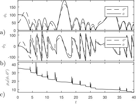 Figure 1