Fractional Burgers wave equation
Ljubica Oparnica, Du\v{s}an Zorica, Aleksandar Okuka

TL;DR
This paper develops and solves fractional Burgers wave equations for viscoelastic media, revealing how different model parameters influence wave speed and propagation characteristics.
Contribution
It introduces two classes of thermodynamically consistent fractional Burgers models and derives their analytical solutions using integral transforms.
Findings
First class exhibits infinite wave propagation speed.
Second class exhibits finite wave propagation speed.
Spatial profiles show unexpected features in wave behavior.
Abstract
Thermodynamically consistent fractional Burgers constitutive models for viscoelastic media, divided into two classes according to model behavior in stress relaxation and creep tests near the initial time instant, are coupled with the equation of motion and strain forming the fractional Burgers wave equations. Cauchy problem is solved for both classes of Burgers models using integral transform method and analytical solution is obtained as a convolution of the solution kernels and initial data. The form of solution kernel is found to be dependent on model parameters, while its support properties implied infinite wave propagation speed for the first class and finite for the second class. Spatial profiles corresponding to the initial Dirac delta displacement with zero initial velocity display features which are not expected in wave propagation behavior.
Click any figure to enlarge with its caption.
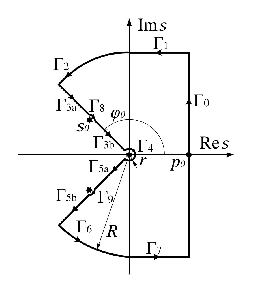 Figure 1
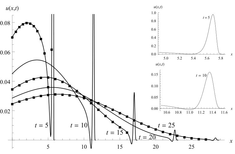 Figure 2
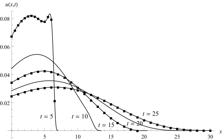 Figure 3
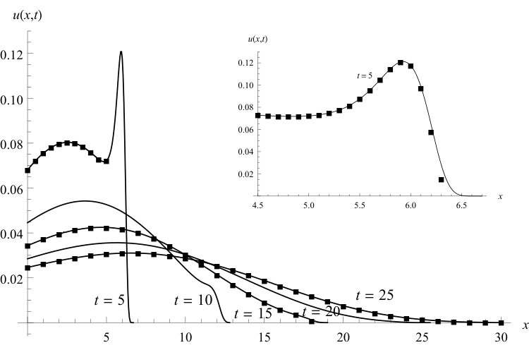 Figure 4
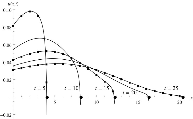 Figure 5
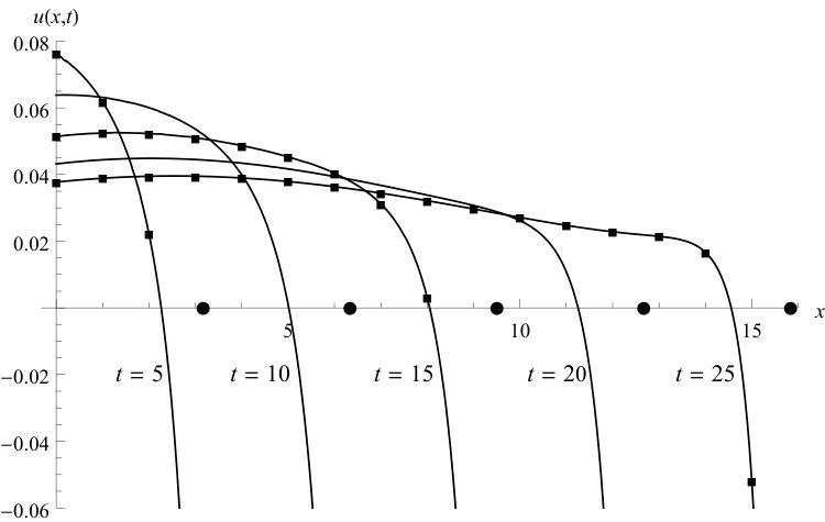 Figure 6
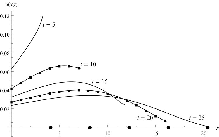 Figure 7
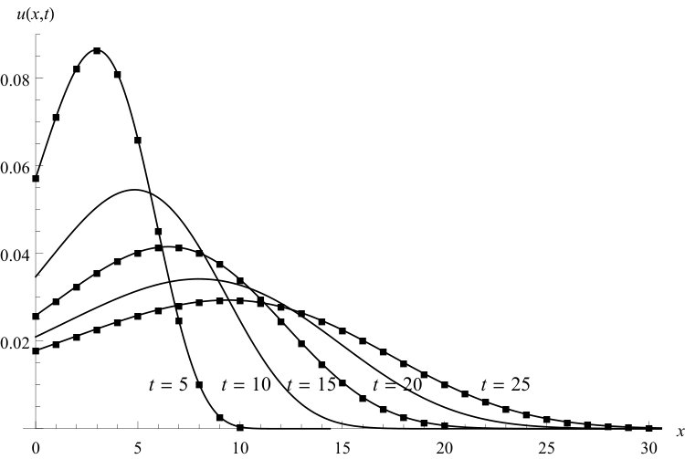 Figure 8
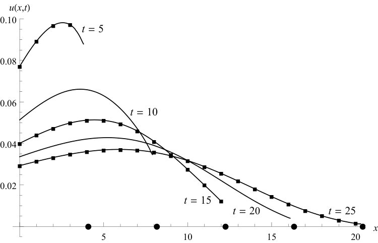 Figure 9
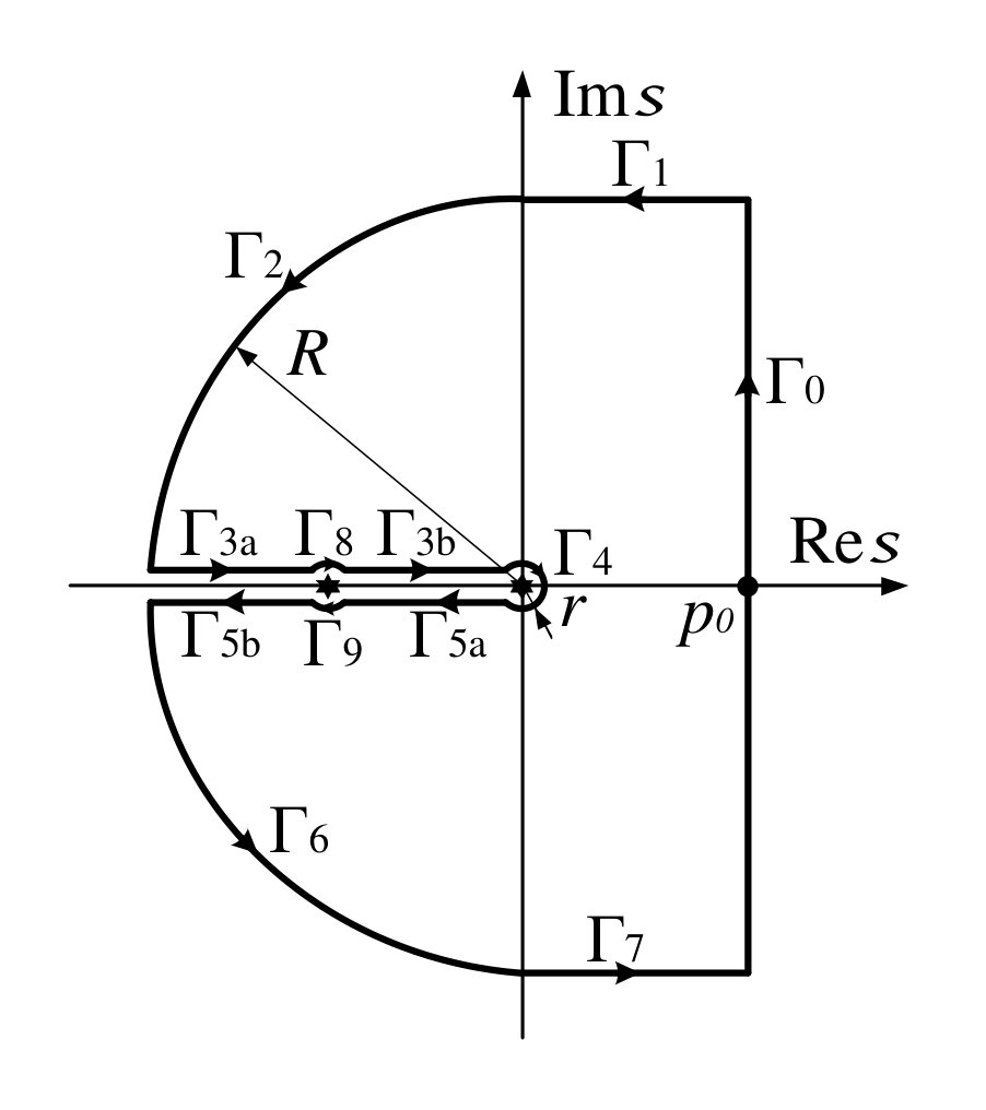 Figure 10
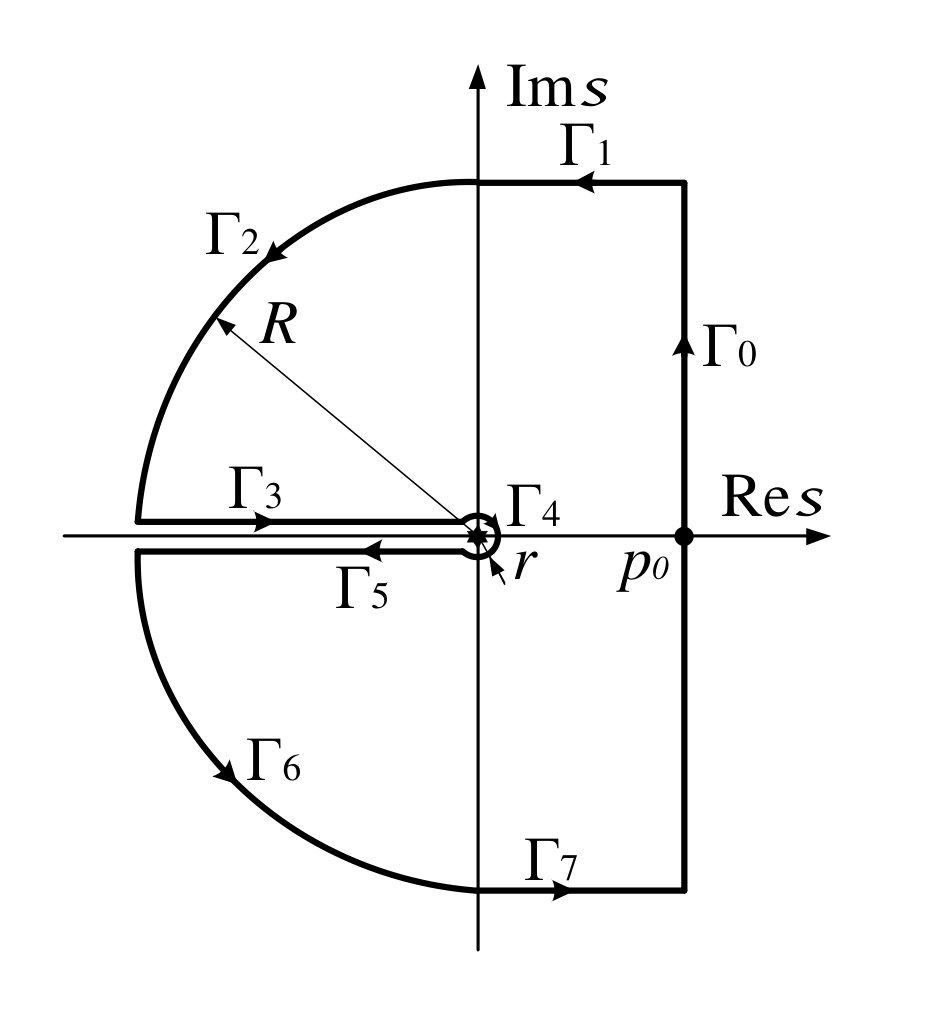 Figure 11
Peer Reviews
No public reviews on file for this paper yet. If you reviewed it on a platform where reviews are public (OpenReview, ICLR, NeurIPS, ICML), you can paste yours below so the community can read it here.
Videos
No videos yet. Explain this paper in a talk, walkthrough, or lecture? Add one.
Fractional Burgers wave equation
Ljubica Oparnica, Dušan Zorica, Aleksandar S. Okuka
Faculty of Education, University of Novi Sad, Podgorička 4, 25000 Sombor, Serbia and Department of Mathematics: Analysis, Logic and Discrete Mathematics, University of Gent, Krijgslaan 281 (building S8), 9000 Gent, Belgium, [email protected] Mathematical Institute, Serbian Academy of Arts and Sciences, Kneza Mihaila 36, 11000 Belgrade, Serbia and Department of Physics, Faculty of Sciences, University of Novi Sad, Trg D. Obradovića 4, 21000 Novi Sad, Serbia, [email protected] Department of Mechanics, Faculty of Technical Sciences, University of Novi Sad, Trg D. Obradovića 6, 21000 Novi Sad, Serbia, [email protected]
Abstract
Thermodynamically consistent fractional Burgers constitutive models for viscoelastic media, divided into two classes according to model behavior in stress relaxation and creep tests near the initial time instant, are coupled with the equation of motion and strain forming the fractional Burgers wave equations. Cauchy problem is solved for both classes of Burgers models using integral transform method and analytical solution is obtained as a convolution of the solution kernels and initial data. The form of solution kernel is found to be dependent on model parameters, while its support properties implied infinite wave propagation speed for the first class and finite for the second class. Spatial profiles corresponding to the initial Dirac delta displacement with zero initial velocity display features which are not expected in wave propagation behavior.
Key words: thermodynamically consistent fractional Burgers models, fractional Burgers wave equation, wave propagation speed
1 Introduction
Fractional Burgers wave equation is written as the system of equations consisting of: equation of motion corresponding to one-dimensional deformable body
[TABLE]
where and are displacement and stress, while is constant material density; strain for small local deformations
[TABLE]
and constitutive equation represented by the fractional Burgers model
[TABLE]
having model parameters assumed as: with and while the operator of Riemann-Liouville fractional derivative of order is defined by
[TABLE]
see [19], where denotes the convolution in time:
In order to solve the Cauchy problem on the real line and the system of governing equations (1), (2), and (3) is subject to initial and boundary conditions:
[TABLE]
where is the initial displacement and is the initial velocity.
Considering the rheological scheme of the classical Burgers model, with the dash-pot element replaced by the Scott-Blair (fractional) element, the fractional Burgers model (3) is derived in [27]. Moreover, using the requirement of storage and loss modulus non-negativity, the analysis of thermodynamical consistency for fractional Burgers model (3), conducted in [27], yielded that the orders of fractional derivatives cannot be independent of the orders of fractional derivatives and this led to formulation of eight thermodynamically consistent fractional Burgers models, divided into two classes.
The first class contains five models, written as
[TABLE]
in an unified manner, such that the highest fractional differentiation order of strain is with while the highest fractional differentiation order of stress is either in the case of Model I, with and or in the case of Models II - V, with and . The fractional differentiation order of stress is less than the differentiation order of strain regardless on the interval or
The second class contains three models, written as
[TABLE]
in an unified manner, such that and with in the case of Model VI; in the case of Model VII; and and in the case of Model VIII. Considering the interval the highest fractional differentiation orders of stress and strain are equal, which also holds true for the orders from interval
The responses in creep and stress relaxation tests for Models I - VIII are examined in [28]. Recall, creep compliance (relaxation modulus ) is the strain (stress) history function obtained as a response to the stress (strain) assumed as the Heaviside step function. It is found that models’ behavior near the initial time-instant is different for the first and the second model class: Models I - V have zero glass compliance, i.e., and thus infinite glass modulus, i.e., while Models VI - VIII have non-zero glass compliance implying the non-zero glass modulus as well. On the other hand, the equilibrium compliance is infinite, i.e., , so that the equilibrium modulus is zero, i.e., for both model classes and therefore all fractional Burgers models describe fluid-like materials. Note, if the equilibrium compliance is finite, then model would represent the solid-like material.
The implication, proved in the present work, is that fluid-like Burgers models belonging to the first class have infinite, while the ones belonging to the second class have finite wave propagation speed
[TABLE]
as in the case of thermodynamically consistent fractional models arising from the general fractional linear model
[TABLE]
obtained and analyzed in [2] for thermodynamical consistency and used in [22] as constitutive equations in wave propagation modeling. Namely, the results of [20, 21], where the wave propagation speed is found via the conic solution support, i.e., in the case of the fractional Zener model and its generalization, respectively given by
[TABLE]
are extended in [22], using the same argumentation as in the previous work, to all four classes of thermodynamically consistent linear fractional models and moreover to the power-type distributed-order model assuming that the orders of fractional differentiation do not exceed one. In particular, it is found that both solid-like and fluid-like materials can have either infinite or finite wave speed. Singularity propagation properties of the memory and non-local type fractional wave equations are investigated in [17, 18] using the tools of microlocal analysis, supporting the results obtained in [20].
Wave propagation phenomena in viscoelastic bodies, modeled by integer and fractional order models, including the question of wave speed and energy dissipation properties are analyzed in [8, 9]. The wavefront expansion of solution, due to Buchen and Mainardi, is introduced in [7] to be later used in [11, 12] when considering the wave equation in viscoelastic materials described by the Bessel as well as by the integer and fractional order Maxwell and Kelvin-Voigt models. The Bessel model for viscoelastic body is introduced in [13] and analyzed in [10]. Features of the wave propagation in viscoelastic media, like the asymptotic behavior of fundamental solution near the wavefront, dispersion, and attenuation is examined in [14, 15, 16]. Wave propagation speed, reinterpreted as the fundamental solution’s peak propagation speed is analyzed in [23, 24, 25]. Modeling viscoelastic materials using the fractional order models, as well as dispersion and attenuation effects described by the corresponding wave equations are reviewed in [26].
Fractional wave equations on bounded and semi-bounded domain are considered in [29, 30, 31] for different fractional models including the Zener, modified Zener, and modified Maxwell models, as well as in [4, 5, 6] in the case of power-type distributed-order model. Generalizations of the classical wave equations and corresponding problems are reviewed in [3, 32].
2 Fractional Burgers model in wave propagation
Fractional Burgers wave equation, as the dimensionless system of equations:
[TABLE]
and either
[TABLE]
for the first class of Burgers models, or
[TABLE]
for the second class of Burgers models, subject to initial and boundary conditions
[TABLE]
is obtained by introducing dimensionless quantities
[TABLE]
with and for the first class of Burgers models, and for the second class, and into system of governing equations (1), (2) and either (6) or (7), subject to (4), (5), and by subsequent omittance of bars.
Models in dimensionless form, along with the corresponding thermodynamical restrictions, are listed below.
Model I:
[TABLE]
with
Model II:
[TABLE]
Model III:
[TABLE]
Model IV:
[TABLE]
Model V:
[TABLE]
Model VI:
[TABLE]
Model VII:
[TABLE]
Model VIII:
[TABLE]
Application of the Fourier transform with respect to the spatial coordinate
[TABLE]
and Laplace transform with respect to the time
[TABLE]
with initial (13) and boundary conditions (14) taken into account, transforms the system of governing equations (10) and either (11), or (12) into ( )
[TABLE]
with either
[TABLE]
in the case of the first class of Burgers equation (11), or
[TABLE]
in the case of the second class of Burgers equation (11).
It is obtained that
[TABLE]
with
[TABLE]
once the system of equations (31), (32) is solved with respect to displacement , implying the solution to the fractional Burgers equation (10) and either (11), or (12), subject to (13) and (14), in the form
[TABLE]
where denotes the convolution with respect to the spatial variable: after inverting Fourier and Laplace transforms in (35).
In order to calculate the solution kernel the inversion of the Fourier transform is performed in (36) using a well-known inversion formula
[TABLE]
implying
[TABLE]
provided that
[TABLE]
which holds for all Models I - VIII, as proved in Appendix A. Further, inverting the Laplace transformation in (39) by the definition
[TABLE]
where is the Bromwich path, the two forms of solution kernel are obtained in Appendix B depending on the number and position of branching points of function given by (39), originating from the zeros of function since except for has no other zeros in the principal Riemann plane, with and given by either (33) or (34). There are three possible cases, since, as shown in [28], function can have no zeros, one negative real zero, or a pair of complex conjugated zeros having negative real part. However, the solution kernel has the same form in the first two cases, thus merged into Case 1 below, while the form of the solution kernel differs in the third case, thus being labeled as Case 2.
Case 1. If function except for either has no branching points, or has a negative real branching point, then function is found as
[TABLE]
either having support in for the first class of fractional Burgers models, or having support in the conic domain for the second class.
Case 2. If function except for has a pair of complex conjugated branching points with negative real part: and , then function is found as
[TABLE]
either having support in for the first class of fractional Burgers models, or having support in the conic domain for the second class.
The solution support properties, in both cases of solution kernel, define the wave propagation speed: infinite if the support is obtained for the first class of Burgers models, and finite if the support is conic domain obtained as
[TABLE]
for the second class of Burgers models. Since see [28, Eq. (57)], the wave propagation speed (44) is exactly the wave propagation speed (8) that is obtained in [22] for the constitutive models having fractional differentiation orders not exceeding one.
3 Numerical examples
Spatial profiles of the solution to the fractional Burgers wave equations, written as the system of equations (10) and either (11), or (12), subject to initial and boundary conditions (13) and (14), with the initial displacement being the Dirac delta distribution and initial velocity being zero, i.e., and implying that the solution is equal to the solution kernel are depicted in Figures 1, 2, and 3 for Model V, representing the first class of fractional Burgers models and in Figures 4, 5, and 6 for Model VII, representing the second class. Recall, in the case of constitutive models belonging to the first class the wave propagation speed is infinite, while in the case of the second class the speed is finite and given by (8). Spatial profiles produced by using the analytical formula for solution kernel given by either (42), or (43), are compared with the solution kernel numerically calculated by the fixed Talbot numerical Laplace inversion Mathematica function, developed by J. Abate and P. P. Valkó according to [1] and available at: http://library.wolfram.com/infocenter/MathSource/4738/. In each of the numerical examples good agreement between profiles obtained by these two methods is found.
Figures 1, 2, and 3 present spatial profiles for Model V in cases when function given by (39), except for does not have other branching points, has one negative real, and has a pair of complex conjugated branching points, respectively. Different number and position of the branching points is a consequence of the change of a single parameter Apart from the main peak originating from the propagation of the initial Dirac delta displacement, there is a noticeable additional peak that is more prominent for small times and ceasing as time passes. As the parameter increases, the change of the nature (number and position) of the branching points from no branching points to a pair of complex conjugated ones, implies the growth of prominence of the additional peak. During the propagation, due to the energy dissipation, height of the main peak decreases, while the width of profile is increasing, while propagation itself is rather slow.
Wave propagation speed is finite for the second class of fractional Burgers models, and in Figures 4, 5, and 6, presenting spatial profiles for Model VII, it is underlined by denoting the ending points of solution support by circles. It is also noticeable that during the propagation, due to the energy dissipation, height of the peak decreases, while its width increases.
Figure 4 presents spatial profiles depending on the nature of the branching points, different than of function given by (39) in three cases obtained as a consequence of changing parameter : Figure 4a represents case when there are no other branching points, Figure 4b when there is one negative real branching point, and Figure 4c when there is a pair of complex conjugated branching points. For small times, the profile shapes are considerably different, while as time passes the profile shapes become alike. In all cases there are jumps at the ending points of solution support: in Figures 4a and 4b displacement jumps from a positive value to zero, while in Figure 4c displacement jumps from a negative value to zero.
When compared to the profiles from Figure 4a, where the displacement jumps to zero at the ending point of solution support, the displacements plotted in Figure 5, representing also the case when there are no other branching points than tend smoothly to zero at the ending points of solution support. Profiles from Figure 5 are similar to the profiles obtained in [20, 21, 22] for fractional constitutive models used wave propagation modeling in viscoelastic dissipative media.
Figure 6 presents spatial profiles in another case of model parameters yielding existence of a pair of complex conjugated branching points (apart of ) which differ from the ones presented in Figure 4c, since it seems that peaks are situated at zero, while displacement seems to converge to infinity at the ending point of solution support.
4 Conclusion
Fractional Burgers wave equations, considered as a dimensionless system of: equation of motion and strain (10), coupled with the constitutive Burgers models either of the first class (11), or of the second class (12), are solved for the Cauchy initial value problem and their solutions as a response to the initial Dirac delta displacement with zero initial velocity are qualitatively analyzed through numerical examples. The method of Fourier, with respect to space, and Laplace transform with respect to time are used in order to obtain analytical solution as a convolution of the solution kernels and initial data. The form of the solution kernel proved to be dependant on model parameters, so that if parameters yield, except for either no branching points, or one negative real branching point of the Laplace transform of solution kernel, then solution kernel takes the form (42), while if, except for the Laplace transform of solution kernel has a pair of complex conjugated branching points, then solution kernel takes the form (43).
Arising from the solution support properties, in both cases of solution kernel, the infinite wave propagation speed is obtained for the first class of Burgers models and finite for the second class. Moreover, the obtained wave propagation speed is consistent with the one obtained for the wave equations involving fractional linear models with differentiation orders below one.
Qualitative analysis has shown the dissipative behavior for both classes of Burgers wave equations, as expected from thermodynamically consistent constitutive laws for viscoelastic body. However, spatial profile shapes differs for the different nature of the branching points. The features of spatial profiles include the jumps from finite value of displacement to zero at the ending points of solution support, as well as profiles that are not expected in wave propagation behavior, like occurrence of the additional peaks and peaks situated at zero.
Appendix A Justification for using the Fourier inversion formula
The solution kernel is obtained by the Fourier and Laplace transforms as (36), and in order to apply the Fourier transform inversion formula (38), the condition (40), i.e.,
[TABLE]
must be fulfilled.
Functions and given by (33) in the case of the first, or by (34) in the case of the second model class, are never zero for Namely, it is well-known that function except for does not have other zeros in the principal Riemann branch while for function it is proved in [28] that if it has zeros, then they lie in the left complex half-plane.
Therefore, it is left to prove that
[TABLE]
It is clear that if then
[TABLE]
Further, by substituting into (45) one obtains
[TABLE]
with
[TABLE]
that will for each fractional Burgers model prove to be strictly positive if implying that given by (45) cannot be zero for Since note that if
Model I
is obtained for so that function given by (46), reads
[TABLE]
The thermodynamical restrictions (16) imply the positivity of all terms in (50), yielding if
Model II
is obtained for and so that function given by (46), reads
[TABLE]
Consider function and its first derivative :
[TABLE]
on the interval Let Since function is monotonically increasing for one has implying that function is an increasing function on the same interval and therefore
[TABLE]
The thermodynamical restriction (18) yields so that by setting and in function given by (52), using (53) one has
[TABLE]
Therefore, again by (18), one has that which, along with the positivity of all other terms in (51), implies that if
Model III
is obtained for and so that function given by (46), reads
[TABLE]
The thermodynamical restriction (20) yields so that by setting and in function given by (52), using (53) one has
[TABLE]
Therefore, again by (20), one has that which, along with the positivity of all other terms in (54), implies that if
Model IV
is obtained for and so that function given by (46), reads
[TABLE]
The thermodynamical restriction (22) yields so that by setting and in function given by (52), using (53) one has
[TABLE]
Therefore, again by (22), one has that which, along with the positivity of all other terms in (55), implies that if
Model V
is obtained for and so that function given by (46), reads
[TABLE]
The thermodynamical restriction (24) yields so that by setting and in function given by (52), using (53) one has
[TABLE]
Therefore, again by (24), one has that which, along with the positivity of all other terms in (56), implies that if
Model VI
is obtained for and so that function given by (46), reads
[TABLE]
The thermodynamical restriction (26) yields which, along with the positivity of all other terms in (57), implies that if
Model VII
is obtained for and so that function given by (46), reads
[TABLE]
The thermodynamical restriction (28) yields which, along with the positivity of all other terms in (58), implies that if
Model VIII
is obtained for and so that function given by (46), reads
[TABLE]
The thermodynamical restriction (30) yields which, along with the positivity of all other terms in (59), implies that if
Appendix B Calculation of the solution kernel
In order to obtain the solution kernels, given by (42) and (43), the inverse Laplace transform (41) will be calculated using the Cauchy integral formula
[TABLE]
where is a closed curve containing the Bromwich path from the Laplace inversion formula (41) and chosen differently depending on the number and position of the branching points of function given by (39).
Branching points of function are points in which the function under the square root is zero, i.e., in (39) either or with and given by (33) in the case of the first or by (34) in the case of the second model class. Function except for does not have other zeros in the principal Riemann plane since
[TABLE]
as proved in [22]. Zeros of function
[TABLE]
with and are analyzed in [28], where it is found that if then function has no zeros in the complex plane, which is valid for Model I, while if then the number and position of zeros of function is as follows:
[TABLE]
where
[TABLE]
with determined from i.e.,
[TABLE]
which is valid for Models II - VII. In the case of Model VIII, zeros of function
[TABLE]
are as follows:
[TABLE]
with determined by
[TABLE]
Note that the branching point is due to the differentiation of fractional order and that function does not have any singularities other than branching points, justifying the use of the Cauchy integral formula.
B.1 Case 1.
Function except for has no other
branching points
If function (39), except for has no other branching points, then the contour appearing in the Cauchy integral formula (60) is chosen as in Figure 7 and parametrized as in Table 1.
[TABLE]
The integrals along contours and calculated as
[TABLE]
yield the solution kernel in the form (42) when used in the Cauchy integral formula (60), since the integrals along all other contours will prove to be zero.
The following estimates will be used. According to (33), respectively (34), after the substitution is made, it is obtained that
[TABLE]
and therefore
[TABLE]
The integral along contour reads
[TABLE]
and since as one has
[TABLE]
The use of (68) and (71) in (72), due to yields
[TABLE]
for the first model class and choosing
[TABLE]
for the second model class. Similar argumentation is valid for the integral along .
The integral along contour takes the form
[TABLE]
so that
[TABLE]
Using (68) and (71) in (73), due to and for yields
[TABLE]
for in the case of the first model class and
[TABLE]
for the second model class. Similar argumentation is valid for the integral along .
The integral along contour :
[TABLE]
tends to zero when , since
[TABLE]
due to and
[TABLE]
Function except for has a negative real
branching point
If function (39), except for has a negative real branching point determined by (61) or (62), then the contour appearing in the Cauchy integral formula (60) is chosen as in Figure 8 and parametrized as in Table 2.
[TABLE]
The integrals along contours and when and are the same integrals as (63), (64), and (65), thus yielding the solution kernel in the form (42) when used in the Cauchy integral formula (60), since the integrals along contours and already proved to be zero, while the integrals along and will prove to be zero.
Namely, the integral along reads
[TABLE]
so that
[TABLE]
since
[TABLE]
because of being zero of function Similar argumentation is valid for the integral along .
B.2 Case 2.
Function except for has a pair of
complex conjugated branching points
If function except for has a pair of complex conjugated branching points with negative real part: and , then the contour appearing in the Cauchy integral formula (60) is chosen as in Figure 9 and parametrized as in Table 3.
[TABLE]
The solution kernel in the form (43) is obtained when the integrals along contours and calculated as
[TABLE]
are used in the Cauchy integral formula (60), since the integrals along contours and already proved to be zero, while the integrals along and will prove to be zero.
The integral along reads
[TABLE]
so that
[TABLE]
since
[TABLE]
because of being zero of function Similar argumentation is valid for the integral along .
Acknowledgment
This work is supported by the Serbian Ministry of Education, Science and Technological Development under grants and , by the Provincial Secretariat for Higher Education and Scientific Research under grant , as well as by FWO Odysseus project of Michael Ruzhansky.
The reference list from the paper itself. Each links out to its DOI / PubMed record.
- 1[1] J. Abate and P. P. Valkó. Multi-precision Laplace transform inversion. International Journal for Numerical Methods in Engineering , 60:979–993, 2004.
- 2[2] T. M. Atanackovic, S. Konjik, Lj. Oparnica, and D. Zorica. Thermodynamical restrictions and wave propagation for a class of fractional order viscoelastic rods. Abstract and Applied Analysis , 2011:ID 975694–1–32, 2011.
- 3[3] T. M. Atanackovic, S. Pilipovic, B. Stankovic, and D. Zorica. Fractional Calculus with Applications in Mechanics: Wave Propagation, Impact and Variational Principles . Wiley-ISTE, London, 2014.
- 4[4] T. M. Atanackovic, S. Pilipovic, and D. Zorica. Distributed-order fractional wave equation on a finite domain: creep and forced oscillations of a rod. Continuum Mechanics and Thermodynamics , 23:305–318, 2011.
- 5[5] T. M. Atanackovic, S. Pilipovic, and D. Zorica. Distributed-order fractional wave equation on a finite domain. Stress relaxation in a rod. International Journal of Engineering Science , 49:175–190, 2011.
- 6[6] T. M. Atanackovic, S. Pilipovic, and D. Zorica. Forced oscillations of a body attached to a viscoelastic rod of fractional derivative type. International Journal of Engineering Science , 64:54–65, 2013.
- 7[7] P. W. Buchen and F. Mainardi. Asymptotic expansions for transient viscoelastic waves. Journal de mécanique , 14:597–608, 1975.
- 8[8] M. Caputo and F. Mainardi. Linear models of dissipation in anelastic solids. La Rivista del Nuovo Cimento , 1:161–198, 1971.