Exact enumeration approach to first-passage time distribution of non-Markov random walks
Shant Baghram, Farnik Nikakhtar, M. Reza Rahimi Tabar, Sohrab Rahvar,, Ravi K. Sheth, Klaus Lehnertz, Muhammad Sahimi

TL;DR
This paper introduces an exact enumeration method to analytically derive the first-passage time distribution for non-Markov random walks, including fractional Brownian motion, applicable to various scientific fields.
Contribution
It presents a novel exact enumeration approach for calculating FPT distributions in non-Markov processes, extending analytical tools beyond Markovian assumptions.
Findings
Derived exact FPT distribution for non-Markov walks
Applied method to fractional Brownian motion with Hurst exponent H
Demonstrated applicability to physics, biology, and geology phenomena
Abstract
We propose an analytical approach to study non-Markov random walks by employing an exact enumeration method. Using the method, we derive an exact expansion for the first-passage time (FPT) distribution for any continuous, differentiable non-Markov random walk with Gaussian or non-Gaussian multivariate distribution. As an example, we study the FPT distribution of a fractional Brownian motion with a Hurst exponent that describes numerous non-Markov stochastic phenomena in physics, biology and geology, and for which the limit represents a Markov process.
Click any figure to enlarge with its caption.
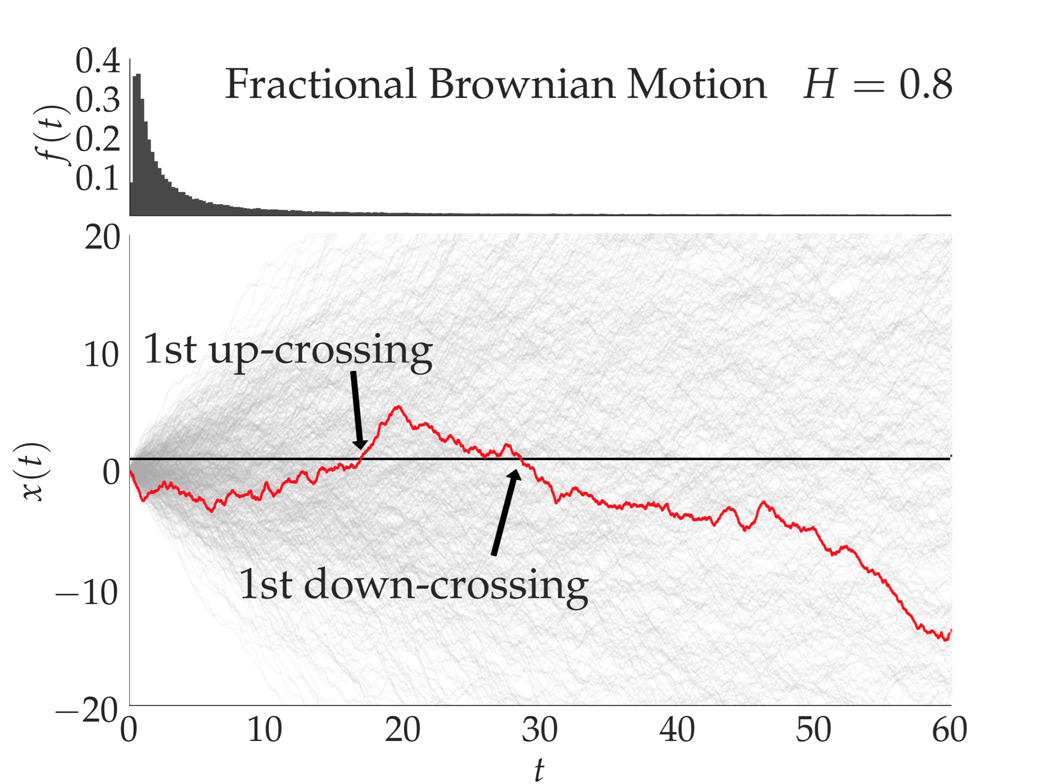 Figure 1
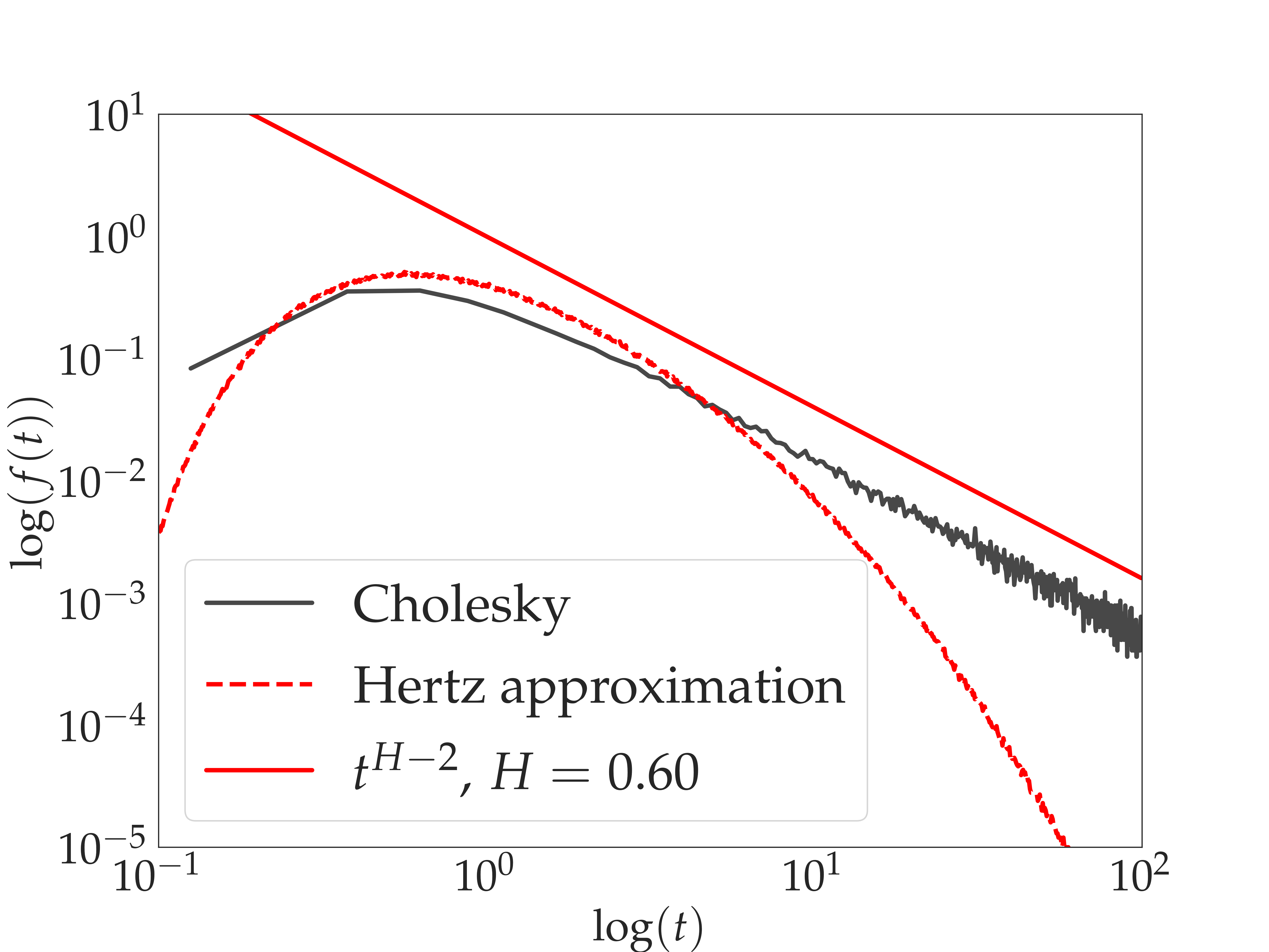 Figure 2
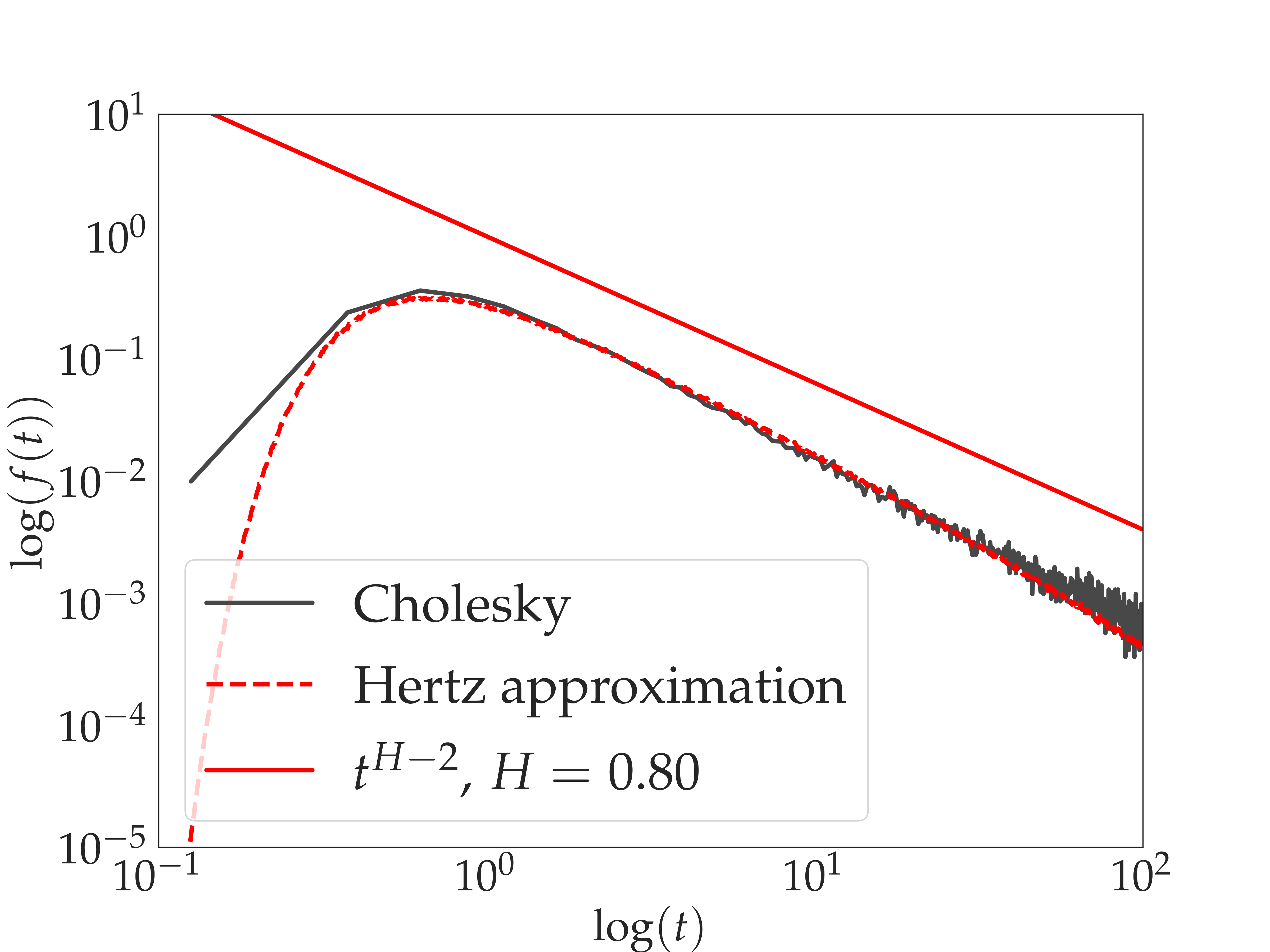 Figure 3
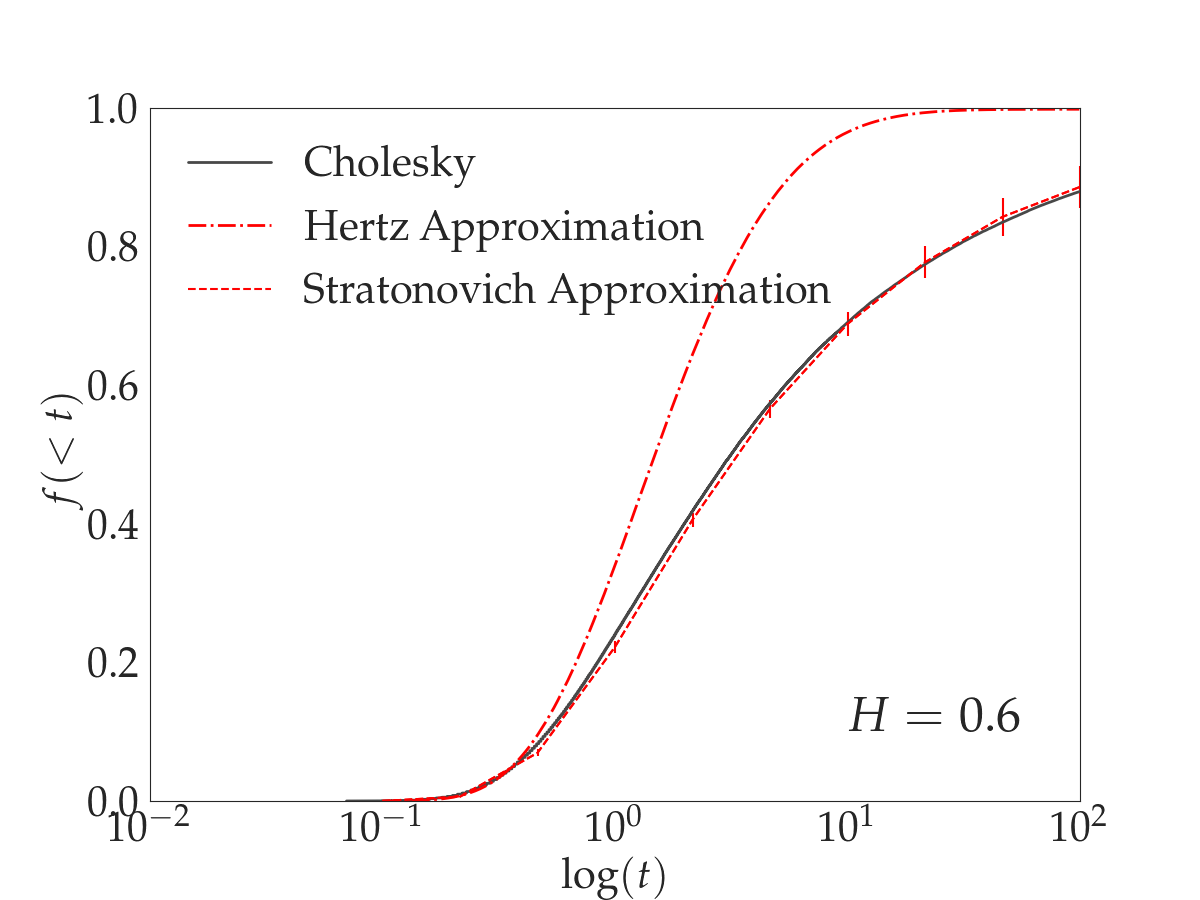 Figure 4
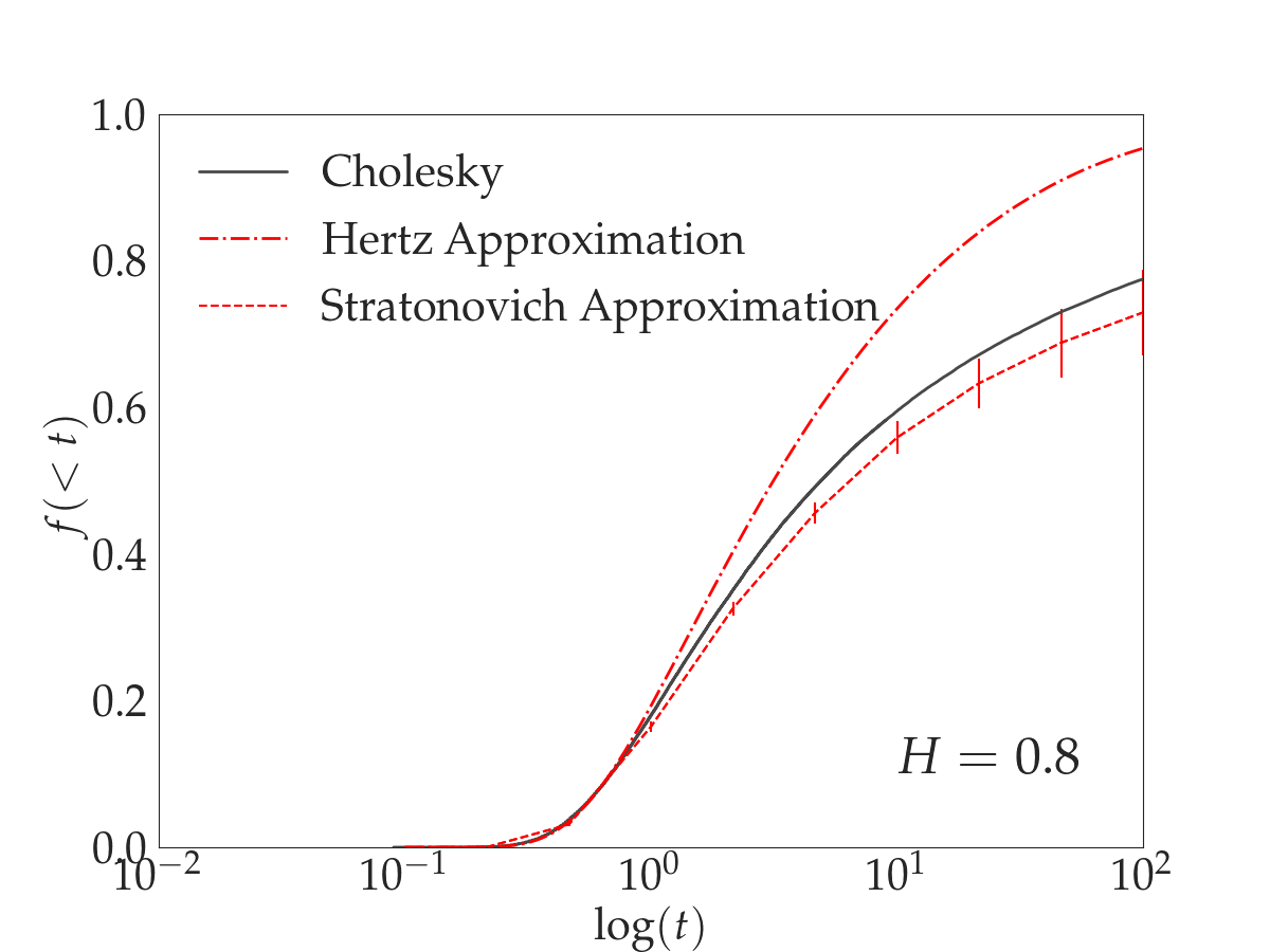 Figure 5
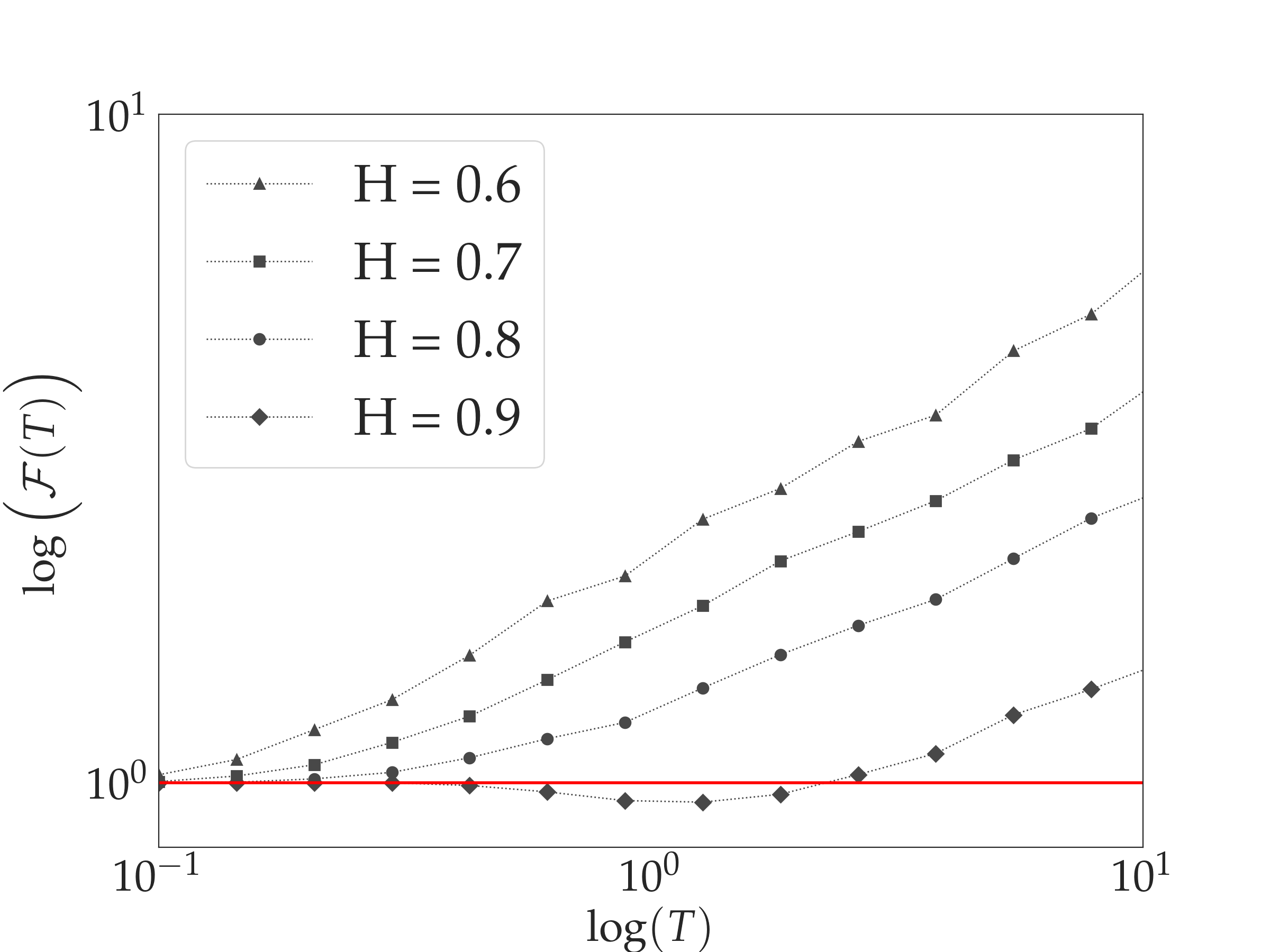 Figure 6
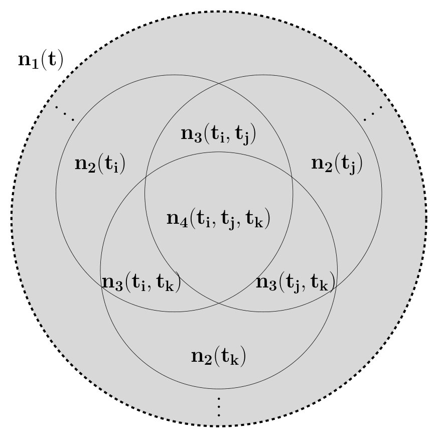 Figure 7
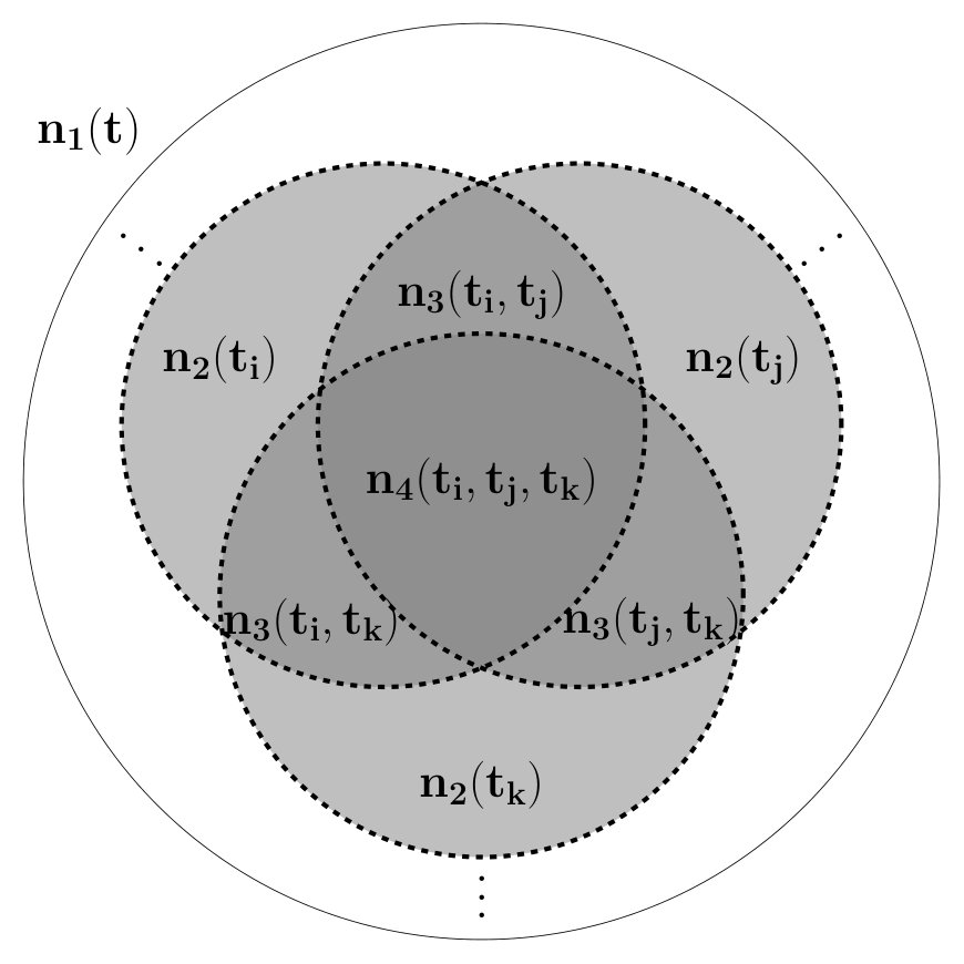 Figure 8
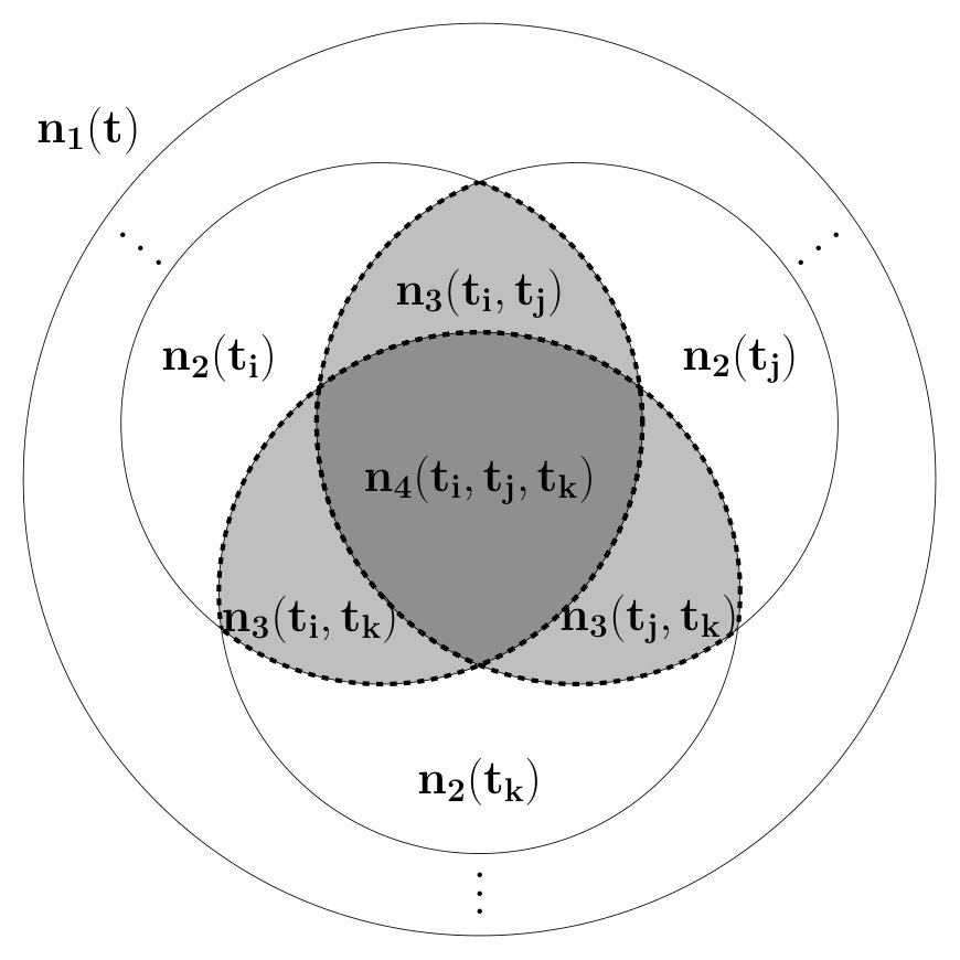 Figure 9
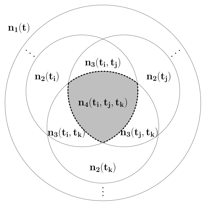 Figure 10
Peer Reviews
No public reviews on file for this paper yet. If you reviewed it on a platform where reviews are public (OpenReview, ICLR, NeurIPS, ICML), you can paste yours below so the community can read it here.
Videos
No videos yet. Explain this paper in a talk, walkthrough, or lecture? Add one.
Exact enumeration approach to first-passage time distribution of non-Markov random walks
Shant Baghram,1, Farnik Nikakhtar,1,2, M. Reza Rahimi Tabar,1,3,† Sohrab Rahvar,1,4 Ravi K. Sheth,2 Klaus Lehnertz,5,6,7 and Muhammad Sahimi8,‡
1*Department of Physics, Sharif University of Technology, Tehran 11155-9161, Iran
2Center for Particle Cosmology, University of Pennsylvania, 209 S. 33rd Street, Philadelphia, PA 19104, USA
3Institute of Physics, Carl von Ossietzky University of Oldenburg, Carl von Ossietzky Straße 9-11, 26111 Oldenburg, Germany
4 Department of Physics, College of Science, Sultan Qaboos University, P.O. Box 36, P.C. 123, Muscat, Sultanate of Oman
5Department of Epileptology, University of Bonn, Sigmund Freud Straße 25, 53105 Bonn, Germany
6Helmholtz Institute for Radiation and Nuclear Physics, University of Bonn, Nussallee 14-16, 53115 Bonn, Germany
7Interdisciplinary Center for Complex Systems, University of Bonn, Brühler Straße 7, 53175 Bonn, Germany
8Mork Family Department of Chemical Engineering and Materials Science, University of Southern California, Los Angeles, California 90089-1211, USA*
We propose an analytical approach to study non-Markov random walks by employing an exact enumeration method. Using the method, we derive an exact expansion for the first-passage time (FPT) distribution for any continuous, differentiable non-Markov random walk with Gaussian or non-Gaussian multivariate distribution. As an example, we study the FPT distribution of a fractional Brownian motion with a Hurst exponent that describes numerous non-Markov stochastic phenomena in physics, biology and geology, and for which the limit represents a Markov process.
I. INTRODUCTION
The concept of first passage refers to the crossing of a prespecified location, or some sort of a threshold, in a stochastic trajectory [1]. The distribution of the first-passage times (FPTs), which represents the probability of crossing the trajectory at a specific time or location [2,3] and depends on the nature of the stochastic process, plays a fundamental role in the theory of stochastic processes, as well as in their applications. The FPT distribution makes it possible to investigate quantitatively the uncertainty in the properties of a stochastic system within a finite time. Two important applications are the extinction time of a disease in the models of epidemic phenomena, and the time for a species to reach a critical threshold in population dynamics. In addition, the statistics of the FPT distribution have many applications to diffusion-limited processes in physics [1], chemistry [4], and biology [5], spreading of electrical blackouts [6], epidemiology [7], and even foraging animals [8,9], as well as to understanding transport processes in disordered materials [10], porous media [11,12], neuroscience [13-16], spreading of computer viruses [17], target search processes [18], economics [19], mathematical finance [20,21], psychology [22], cosmology [23,24], and the reliability theory [25]. Through a suitable boundary the FPT presents the first time that the error in the so-called clock model [26] becomes too large and uncontrollable. Rapid detection of anomalies is closely related to recognizing the optimal stopping time of a diffusion process [27] and, hence, the FPT distribution.
Due to their very large number of applications, the FPT properties have been studied extensively, and are well understood when the stochastic phenomena represent a Markov process. As a general rule, however, the dynamics of a given stochastic process in complex media is the result of its interactions with the environment around it, which may contain trapping sites, obstacles, moving parts, active pumps, etc. [28], and cannot be described as a Markov process. Indeed, although the evolution of the set of all microscopic degrees of freedom of a system is Markovian, the dynamics restricted only to the random walker is not [3,29,30]. Experimental realizations of non-Markov dynamics include diffusion of tracers in crowded narrow channels [31] and in complex fluids, such as nematics [32] and viscoelastic solutions [33,34], as well as the dark matter halo mass function [35]. Even in simple fluids, hydrodynamic memory influences various phenomena and, thus, non-Markov dynamics has been reported recently [36].
Using inclusion-exclusion principle and an exact enumeration method, we derive in this paper the FPT distribution of a non-Markov random walk by assuming that the trajectory of the walk is differentiable at every point. As an example, we derive the FPT distributions of fractional Brownian motion (FBM) with a given Hurst exponent . The analytical results are confirmed by extensive numerical simulation and the analysis of trajectories.
The rest of this paper is organized as follows. In the next section we describe the exact enumeration approach to derive the FPT probability density of a non-Markovian random walk. We then drive in Sec. III an analytical expression for the FPT distribution of FBM. The results of numerical simulations are presented in Sec. IV, while the paper is summarized in Sec. V. In the Appendix, we provide the details of the derivation of our results.
II. EXACT ENUMERATION METHOD FOR THE FPT PROBABILITY DENSITY
We define a general dynamical equation for a random walk, , driven by a correlated, nonstationary noise (velocity) ,
[TABLE]
is assumed to be continuous and its derivative (velocity) to be well-defined at any time [37]. The noise has a zero mean and an arbitrary -point joint distribution . The correlation function depends on both and . Because is a stochastic process, each of its realizations reaches a given barrier for the first time at a different time , giving rise to a FPT probability density . Consider the trajectories with the initial conditions and , crossing the barrier in the time interval and with . The crossing is equivalent to the conditions that and [16,38]. If is constant, will lie in the interval . Then, the probability that satisfies the passage condition is
[TABLE]
where we kept the terms up to the order of . Since at , we should integrate over all positive velocities. Therefore, the probability of crossing the barrier per unit time is given by [16],
[TABLE]
Equation (2) represents the rate of up-crossing, rather than a density function and, thus, it is not normalized. We generalize Eq. (2) to the joint probability of multiple up-crossings, i.e., crossing the barrier in each of the intervals , by integrating over all the crossing points ,
[TABLE]
Using Bayes’ theorem, one may substitute the conditional probability density in Eq. (3) with the joint probability density. In Fig. 1 typical trajectories, as well as the FPT distribution of the FBM for with are presented. The trajectories are constructed using the Cholesky decomposition (see below).
A trajectory can cross several times (see the lower panel of Fig. 1). We relate the FPT distribution to the statistical properties of the up-crossings, which are considered as point processes with rates , where refers to the number of up-crossing. To this end, we look for the fraction of all the trajectories that up-cross for the first time at time with the initial conditions at time , and enumerate them in terms of . To simplify the notation, we drop and the initial conditions.
The rate is over-counted through the trajectories that had an up-crossing at shorter times . Therefore, we subtract their fraction from the first term. This stems from the fact that is a local function in , but there is no guaranty that a trajectory has not up-crossed before . The over-counting implies that the main problem is a combinatorial counting. Thus, as an enumeration technique we use the inclusion-exclusion principle, one of the most useful principles of counting in combinatorics and probability. According to De Morgan’s laws, in the general and complementary form, the principle of inclusion-exclusion for finite sets is expressed by
[TABLE]
where is a finite universal set containing all the , and are the complement of in . That the trajectories cross for the first time at time implies that they should not have been crossed at at shorter times. We consider as the universal set, and define the next subset by , denoting the fraction of trajectories for which the up-crossing at time is not for the first time, and that they had a previous up-crossing at a shorter time . Then, the FPT distribution is given by, , because only the trajectories that have a first up-crossing at time and do not belong to the subsets are of interest. Using Eq. (4), we obtain the FPT distribution [16]:
[TABLE]
where are given by the conditional probabilities (3). The factor accounts for the number of permutations of the variables , with the signs explained in Table I. To calculate , we consider the trajectories in the absence of and let them return after an up-crossing and, then, up-cross the barrier times. The correct counting of such multiple crossings yields the distribution of the FPT. Equation (5) provides us with the exact expansion of the FPT distribution for any continuous, differentiable non-Markov random walk with Gaussian or non-Gaussian multivariate distribution [16]. We note that a naive truncation of the series would give rise to a non-normalized (diverging in the long-time limit) distribution [39].
Let us define as a point process the time scales at which the trajectories cross . The distributions of such a point process are the aforementioned rate functions. Since the trajectories have nonzero velocities, successive up-crossings cannot be too close, so that is zero if two of its arguments are equal. Such point processes represent systems of nonapproaching random points [40]. There are two types of decoupling approximations to deal with the infinite series in Eq. (5), which are based on approximating the higher-order terms by the lower-order ones and are known as the Hertz and Stratonovich approximations. The general expression for is given by
[TABLE]
The Hertz approximation is based on assuming that all the up-crossings are independent of each other, and that the correlations between them are negligible. This leads to the following FPT distribution with [24,39,41]:
[TABLE]
In the Hertz approximation factorizes to . In the Stratonovich approximation, we calculate exactly the first and the second terms of the expansion and approximate all the higher-order terms by the first two [35], with the corresponding FPT distribution being in the form of Eq. (6) with [39],
[TABLE]
where . For simplicity and in order to derive an expression for , we assume in the following that the velocity distribution is Gaussian.
III. ANALYTICAL DERIVATION OF THE FPT DISTRIBUTION OF THE FBM
We now derive the FPT distribution of the FBM with a Hurst exponent , which is defined in terms of its nonstationary correlation function [42]:
[TABLE]
which is positive semidefinite (see the Appendix) with its first derivative (velocity) being the fractional Gaussian noise (FGN) so that, . Using physical arguments [43,44], as well as rigorous analysis [45], it was shown that the scaling behavior of the FPT distribution of a FBM has the following long-time behavior
[TABLE]
Given that the FBM and FGN have Gaussian distributions for and , respectively, we determine and and, therefore, and the FPT distribution in the Hertz and Stratonovich approximations. It is straightforward to show that is given by the following expression,
[TABLE]
where is a Gaussian distribution with mean and variance , where and . For the FBM, and . In the Appendix, we present an expression for in terms of the Hurst exponent . We find that the explicit expression for is given by
[TABLE]
where . Using Eq. (7) we obtain the FPT distribution in the Hertz approximation, which, in general, is accurate for estimating the first peak of the FPT distribution, but it over- or underestimates its tail. Similarly, we find that,
[TABLE]
where all the distributions in Eq. (12) are Gaussian. For example, has the mean (see the Appendix for the variance)
[TABLE]
The correlation functions and are given by Eq. (A.9) in the Appendix, and . Having and enables one to determine and in the Hertz and Stratonovich approximations.
IV. NUMERICAL RESULTS
Figure 1 presents the trajectories of a FBM process using the Cholesky decomposition [46,47] (see the Appendix) and their FPT distribution for , , and . In Fig. 2 the FPT distributions of the FBM trajectories is plotted. The FPT is obtained from the Cholesky method. In these plots, we also show the FPT distributions in the Hertz approximation, which deviate from the FPT directly computed using trajectories. For comparison, the theoretically-predicted tails of the distributions, i.e., , are also plotted. Figure 2 indicates that the theoretical tails of the FPT in the long-time limit coincide with the FPT distributions computed using the trajectories. As already mentioned above the Hertz approximation predicts correctly the location of the peak of the FPT distribution, but underestimates the tails.
To derive the FTP distribution in the Stratonovich approximation with , one must calculate via Eq. (9), and then use Eq. (6). To avoid any error from the numerical differentiation of , we determine the integrated FPT distribution via the term . In Fig. 3 the cumulative FPT distribution is presented for and , indicating that the Hertz approximation deviates clearly from the results computed via the Cholesky decomposition. As shown in Fig. 2, the tail of in the Hertz approximation does not coincide completely with those obtained by the Cholesky decomposition. Higher-order approximations, e.g., the Stratonovich approximation, are therefore needed, implying that should not be factorized as . As shown in Fig. 3, the Stratonovich approximation provides better estimations for the FPT distributions.
One may define various measures to study the interdependence of the up-crossing events. The simplest measure is the Fano factor. Consider a time window and count the mean number (and its variance) of up-crossing events for trajectories in the window. The Fano factor is defined as the variance of the number of up-crossing events in , divided by its mean number, and is written in terms of and [48]. More specifically, the Fano factor is given by (with ), where and [48]. For independent point processes, i.e., , one has . Therefore, for a Poisson process . By definition, and refer, respectively, to over- and under-dispersion [49]. We plot in Fig. 4 the Fano factor versus the size of the time window , which indicates that, in the long-time limit, the up-crossing point processes are strongly over-dispersed. This means that in such time scales should not be factorized as , and that the Hertz approximation is not appropriate for estimating the tails of the FPT distribution. A very crucial point to indicate is that in the time span which the Hertz approximation works well and it is very near to the Cholesky-derived FPT distribution. On the other and if the Fano factor deviates from unity, it is certain that the Hertz approximation is not suitable for FPT, however this parameter can not quantify the accuracy of Stratonovich approximation.
V. SUMMARY
Except for the limiting case of Markov processes, no exact analytical expression for the FPT distribution of general non-Markov random walks had been derived. In principle, the FPT distribution of non-Markov processes may be obtained from the solution of the associated Fokker-Planck equation with absorbing boundaries in higher dimensions, resulting from the Markovian embedding of a non-Markov process [50]. Even the calculation of the mean FPT for a non-Markov process is, however, a rather difficult task, since the corresponding boundary problem cannot be treated in a straightforward manner [51-55]. We presented a general method for deriving such analytical expressions for the FPT distribution. This is done by using an exact enumeration method based on combinatorics and the inclusion-exclusion principle, which can be generalized to include the FTP distribution of non-Markov random walks in higher dimensions. As an example, analytical results were presented for the FBM with the Hurst exponent , which is a non-Markov process with infinite-range memory, and has wide applications in many disciplines [28]. The numerical results were also compared with two well-known approximations, namely, the Hertz and Stratonovich approximations, which revealed their shortcomings.
ACKNOWLEDGMENTS
S.B. acknowledges the partial support of Sharif University of Technology, Grant No. G960202 for this paper. F.N. acknowledges support from the National Science Foundation Graduate Research Fellowship under Grant No. DGE-1845298.
APPENDIX
We provide the details of the main results presented in the main text of the paper.
A. Variance of the velocity of fractional Brownian motion
The time derivative (increments) of the FBM is the FGN, and has the following correlation function
[TABLE]
where , and . Here, is used for smoothing the FBM to make it numerically differentiable [42]. We note that in the limit , the -dependence of drops out. In the literature [42], there is no unique expression for . Here, by generating the FBM trajectories and numerically differentiating them for , the best fit is found to be , where , , and .
B. Fractional Gaussian noise
The stochastic representation of the FBM is given by,
[TABLE]
where is a Wiener process that is written in terms of the Gaussian white noise as, . The FGN is then defined by, . Taking the time derivative of Eq. (A2) yields
[TABLE]
The second term on the r.h.s. of Eq. (A3) is not finite for . Therefore, the FBM has no well-defined ”velocity” for the Hurst exponent in the range of .
C. Proof for the variance of the FBM being positive semidefinite
A symmetric real matrix C is the covariance of some random (Gaussian) vector, if and only if it is positive semidefinite, which means that
[TABLE]
where here is the aforementioned random vector. The FBM has a vanishing mean (), while its covariance is given by Eq. (10) of the main text, for and . We show that
[TABLE]
is a covariance function. Consider the function
[TABLE]
defined for all and , where for all . Since , we can determine and
[TABLE]
where is a positive and finite constant that depends only on . Therefore, we find
[TABLE]
D. Analytical expressions for and with a Gaussian velocity
Due to the linearity of the system, all the joint probability densities are Gaussian and have the form
[TABLE]
Here, is an -dimensional vector whose th component is the coordinate or the velocity at time , and is the symmetric correlation matrix whose entries are the correlation functions between the corresponding components of the vector : . Then, is obtained in closed analytical form:
[TABLE]
where and . For the joint densities of multiple up-crossings no closed expression can be obtained. We evaluate the integral over in Eq. (3) analytically and then perform numerical integration of the resulting expression over to determine . The integrals over time in the expressions for are also evaluated numerically. For , we compute the mean and variance of the conditional distributions,
[TABLE]
Assuming that , the correlations are given by
[TABLE]
where, for example, . We also know that
[TABLE]
Note that all the conditional distributions are Gaussians and, therefore, they are specified by their mean and variance. For example, for we have
[TABLE]
[TABLE]
For , we should calculate the mean and variance of , which are given by
[TABLE]
[TABLE]
Now, for we obtain
[TABLE]
[TABLE]
E. The Cholesky decomposition
To compute the non-Markovian first up-crossing distribution for the FBM, we must generate trajectories with the correct ensemble properties. Here, we describe an algorithm to generate such trajectories. Equation (9) of the main text defined, , the correlation between the between times and . The matrix C is real, symmetric, and positive-definite and, therefore, it has a unique decomposition, , in which L is a lower triangular matrix, which is known as the Cholesky’s decomposition. We use L to generate the ensemble of the trajectories as follows.
First, consider a vector , which is Gaussian white noise with zero mean and unit variance (i.e. ). If we generate the desired trajectories as
[TABLE]
then will have the correlations of random walk given by
[TABLE]
Since L is triangular, only a sum over is needed in matrix calculations, so the method is fast. Next, we provide a proof of the Cholesky decomposition, and present it in terms of the correlation matrix. In a more general context, there is a sufficient condition for a square matrix to have a LU decomposition, , where L and U are, respectively, the lower and upper triangular matrices of C. If all the leading principal minors of the matrix C are nonsingular, then C has an LU decomposition. Let us recall that the th leading principle minor of C is given by
[TABLE]
where we have assumed that are nonsingular. Using induction, it is not difficult to show that there is a LU decomposition for the correlation matrix. Using the symmetry of C, we write
[TABLE]
which implies that
[TABLE]
The l.h.s of the equation is upper triangular, whereas the r.h.s. is a lower triangular matrix. Consequently, there is a diagonal matrix D such that . Then, , which for the correlation matrix implies that, , where D is a positive-definite matrix with its elements also being positive. Accordingly, we write C as , where , which is the Cholesky decomposition.
It is clear that the matrix is a lower triangular matrix as well, and can be used to transform independent normal variables into dependent multinormal variables, which is the main idea of the method we propose to construct the exact trajectories. The matrix is calculated by [40,41]
[TABLE]
where, is a positive-definite correlation matrix, is its inverse, and for , so that . We note that for a semi-positive definite matrix we should remove the first row and first column of the matrix in order to have a positive-definite matrix, and then apply the Cholesky decomposition.
Algorithmically, our Cholesky decomposition algorithm constructs L as follows:
input
for do
\qquad L_{kk}\leftarrow\Big{(}C_{kk}-\displaystyle\sum_{s=1}^{k-1}L_{ks}^{2}\Big{)}^{1/2}
for do
\qquad\qquad L_{ik}\leftarrow\Big{(}C_{ik}-\displaystyle\sum_{s=1}^{k-1}L_{is}L_{ks}\Big{)}\Big{/}L_{kk}
end
end
output
All the trajectories for FBM in this paper were constructed using this algorithm.
- [1]
S. Redner, A Guide to First-Passage Processes (Cambridge University Press, Cambridge, 2001).
- [2]
S. Condamin, O. Bénichou, V. Tejedor, R. Voituriez, and J. Klafter, First-passage times in complex scale-invariant media, Nature 450, 77 (2007).
- [3]
T. Guérin, N. Levernier, O. Bénichou, and R. Voituriez, Mean first-passage times of non-Markovian random walkers in confinement, Nature 534, 356 (2016).
- [4]
S.A. Rice, Diffusion-Limited Reactions, vol. 25 (Elsevier, Amsterdam, 1985).
- [5]
M.J. Saxton, A biological interpretation of transient anomalous subdiffusion. II. Reaction kinetics, Biophys. J. 94, 760 (2008).
- [6]
B.A. Carreras, V.E. Lynch, I. Dobson, and D.E. Newman, Critical points and transitions in an electric power transmission model for cascading failure blackouts, Chaos 12, 985 (2002).
- [7]
A.L. Lloyd and R.M. May, Epidemiology - how viruses spread among computers and people, Science 292, 1316 (2001).
- [8]
O. Benichou, C. Loverdo, M. Moreau, and R. Voituriez, Two-dimensional intermittent search processes: An alternative to Lévy flight strategies, Phys. Rev. E 74, 020102 (2006).
- [9]
G.M. Viswanathan, E.P. Raposo, and M.G.E. da Luz, Lévy flights and superdiffusion in the context of biological encounters and random searches, Phys. Life Rev. 5, 133 (2008).
- [10]
D. Ben-Avraham and S. Havlin, Diffusion and Reactions in Fractals and Disordered Systems (Cambridge University Press, London, 2000).
- [11]
M. Sahimi, H.T. Davis, and L.E. Scriven, Dispersion in disordered porous media, Chem. Eng. Commun. 23, 329 (1983).
- [12]
M. Sahimi, B.D. Hughes, L.E. Scriven, and H.T. Davis, Dispersion in flow through porous media: I. One-phase flow, Chem. Eng. Sci. 41, 2103 (1986).
- [13]
H.C. Tuckwell, Introduction to Theoretical Neurobiology (Cambridge University Press, London, 1988).
- [14]
A.N. Burkitt, A review of the integrate-and-fire neuron model: I. Homogeneous synaptic input, Biol. Cybern. 95, 1 (2006).
- [15]
L. Sacerdote and M.T. Giraudo, in, Stochastic Biomathematical Models, edited by M. Bachar, J. Batzel, and S. Ditlevsen (Springer, New York, 2013), p. 99.
- [16]
T. Verechtchaguina, I.M. Sokolov, and L. Schimansky-Geier, First passage time densities in non-Markovian models with subthreshold oscillations, Europhys. Lett. 73, 691 (2006).
- [17]
R. Pastor-Satorras and A. Vespignani, Epidemic spreading in scale-free networks, Phys. Rev. Lett. 86, 3200 (2001).
- [18]
O. Benichou, M. Coppey, M. Moreau, P.-H. Suet, and R. Voituriez, Optimal search strategies for hidden targets, Phys. Rev. Lett. 94, 198101 (2005).
- [19]
Q. Hu, Y. Wang, and X. Yang, The hitting time density for a reflected Brownian motion, Comput. Econ. 40, 1 (2012).
- [20]
J. Janssen, O. Manca, and R. Manca, Applied Diffusion Processes, from Engineering to Finance (Wiley, New York, 2013).
- [21]
V. Linetsky, Lookback options and diffusion hitting times: A spectral expansion approach, Finance Stoch. 8, 373398 (2004).
- [22]
D.J. Navarro and I.G. Fuss, Fast and accurate calculations for first-passage times in Wiener diffusion models, J. Math. Psych. 53, 222 (2009).
- [23]
M. Musso and R.K. Sheth, The importance of stepping up in the excursion set approach, Mon. Notices R. Astro. Soc. 438, 2683 (2014).
- [24]
M. Musso and R.K. Sheth, The excursion set approach in non-Gaussian random fields, Mon. Notices R. Astr. Soc. 439, 3051 (2014).
- [25]
V. Pieper, M. Domin, and P. Kurth, Level crossing problems and drift reliability, Math. Methods Oper. Res. 45, 347 (1997).
- [26]
C. Zucca and P. Tavella, The clock model and its relationship with the Allan and related variances, IEEE Trans. Ultras. Ferroelectrics and Frequency Control 52, 289 (2005).
- [27]
C. Zucca, P. Tavella, and G. Peskir, Detecting atomic clock frequency trends using an optimal stopping method, Metrologia 53, S89 (2016).
- [28]
I.M. Sokolov, Models of anomalous diffusion in crowded environments, Soft Matter 8, 9043 (2012).
- [29]
R. Friedrich, J. Peinke, M. Sahimi, and M.R. Rahimi Tabar, Approaching complexity by stochastic methods: from biological systems to turbulence, Phys. Rep. 506 87 (2011).
- [30]
M. Anvari, M.R. Rahimi Tabar, J. Peinke, and K. Lehnertz, Disentangling the stochastic behavior of complex time series, Sci. Rep. 6, 35435 (2016).
- [31]
Q.-H. Wei, C. Bechinger, and P. Leiderer, Single-file diffusion of colloids in one-dimensional channels, Science 287, 625 (2000).
- [32]
T. Turiv, I. Lazo, A. Brodin1, B.I. Lev, V. Reiffenrath, V.G. Nazarenko, and O.D. Lavrentovich, Effect of collective molecular reorientations on Brownian motion of colloids in nematic liquid crystals, Science 342, 1351 (2013).
- [33]
D. Ernst, M. Hellmann, J. Köhler, and M. Weiss, Fractional Brownian motion in crowded fluids, Soft Matter 8, 4886 (2012).
- [34]
T.G. Mason and D.A. Weitz, Optical measurements of frequency-dependent linear viscoelastic moduli of complex fluids, Phys. Rev. Lett. 74, 1250 (1995).
- [35]
F. Nikakhtar, M. Ayromlou, S. Baghram, S. Rahvar, M.R. Rahimi Tabar, and R.K. Sheth, The excursion set approach: Stratonovich approximation and Cholesky decomposition, Mon. Notices R. Astro. Soc. 478, 4, 5296 (2018).
- [36]
T. Franosch, M. Grimm, M. Belushkin, F.M. Mor, G. Foffi, L. Forró, and S. Jeney, Resonances arising from hydrodynamic memory in Brownian motion, Nature 478, 85 (2011).
- [37]
M. Scott, Applied Stochastic Processes in Science and Engineering (Springer, Berlin, 2013).
- [38]
G.R. Jafari, M.S. Movahed, S.M. Fazeli, M.R. Rahimi Tabar, and S.F. Masoudi, Level crossing analysis of the stock markets, J. Stat. Mech. 06, P06008 (2006).
- [39]
T. Verechtchaguina, I.M. Sokolov, and L. Schimansky-Geier, First passage time densities in resonate-and-fire models, Phys. Rev. E 73, 031108 (2006).
- [40]
R. Stratonovich, Topics in the Theory of Random Noise, Vol. 2 (Taylor & Francis, London, 1967).
- [41]
P. Hertz, Uber den gegenseitigen durchschnittlichen Abstand von Punkten, die mit bekannter mittlerer Dichte im Raume angeordnet sind, Mathematische Annalen 67, 387 (1909).
- [42]
B.B. Mandelbrot and J.W. van Ness, Fractional Brownian motions, fractional Gaussian noises and applications, SIAM Rev. 10, 422 (1968).
- [43]
M. Ding and W. Yang, Distribution of the first return time in fractional Brownian motion and its application to the study of on-off intermittency, Phys. Rev. E 5, 207 (1995).
- [44]
J. Krug, H. Kallabis, S.N. Majumdar, S. Cornell, A.J. Bray, and C. Sire, Persistence exponents for fluctuating interfaces, Phys. Rev. E 56, 2702 (1997).
- [45]
G. M. Molchan, Maximum of a fractional Brownian motion: probabilities of small values, Commun. Math. Phys. 205, 97 (1999).
- [46]
J.E. Gentle, Numerical Linear Algebra for Applications in Statistics (Springer, Berlin, 1998), p. 93.
- [47]
V. Madar, Direct formulation to Cholesky decomposition of a general nonsingular correlation matrix, Stat. Probab. Lett. 103, 142 (2015).
- [48]
T. Engel, Firing Statistics in Neurons as Non-Markovian First Passage Time Problem, Ph.D. Thesis, Humboldt-Universität zu Berlin (2006).
- [49]
D.R. Cox and V. Isham, Point Processes (Chapman & Hall, London, 1980).
- [50]
P. Hänggi, P. Talkner, and M. Borkovec, Reaction-rate theory: fifty years after Kramers, Rev. Mod. Phys. 62, 251 (1990).
- [51]
C.R. Doering, P.S. Hagan, and C.D. Levermore, Bistability driven by weakly colored Gaussian noise: The Fokker-Planck boundary layer and mean first-passage times, Phys. Rev. Lett. 59, 2129 (1987).
- [52]
P. Hänggi, P. Jung, and P. Talkner, Comment on “Bistability driven by weakly colored Gaussian noise: The Fokker-Planck boundary layer and mean first-passage times,” Phys. Rev. Lett. 60, 2804 (1988).
- [53]
R. Graham and T. Tél, Nonequilibrium potential for coexisting attractors, Phys. Rev. A 33, 1322 (1986).
- [54]
M.I. Dykman, P.V.E. McClintock, V.N. Smelyanski, N.D. Stein, and N.G. Stocks, Optimal paths and the prehistory problem for large fluctuations in noise-driven systems, Phys. Rev. Lett. 68, 2718 (1992).
- [55]
S.M. Soskin, Large fluctuations in multiattractor systems and the generalized Kramers problem, J. Stat. Phys. 97, 609 (1999).
Table I: The exact enumeration method. The th column corresponds to the th term of the sum in Eq. (5).
[TABLE]