Combination of searches for Higgs boson pairs in $pp$ collisions at $\sqrt{s} = $13 TeV with the ATLAS detector
ATLAS Collaboration

TL;DR
This paper combines multiple searches for Higgs boson pair production at 13 TeV with the ATLAS detector, setting limits on production cross-sections, Higgs self-coupling, and new physics models, with no significant excess observed.
Contribution
It provides the first combined analysis of various Higgs pair decay channels at 13 TeV, improving constraints on Higgs self-coupling and new physics scenarios.
Findings
No significant excess above Standard Model predictions.
Limits set on Higgs pair production cross-section and self-coupling.
Constraints on new physics models like resonances and extra dimensions.
Abstract
This letter presents a combination of searches for Higgs boson pair production using up to 36.1 fb of proton-proton collision data at a centre-of-mass energy TeV recorded with the ATLAS detector at the LHC. The combination is performed using six analyses searching for Higgs boson pairs decaying into the bbbb, bbWW, bb, WWWW, bb and WW final states. Results are presented for non-resonant and resonant Higgs boson pair production modes. No statistically significant excess in data above the Standard Model predictions is found. The combined observed (expected) limit at 95% confidence level on the non-resonant Higgs boson pair production cross-section is 6.9 (10) times the predicted Standard Model cross-section. Limits are also set on the ratio () of the Higgs boson self-coupling to its Standard Model value.…
Click any figure to enlarge with its caption.
 Figure 1
 Figure 2
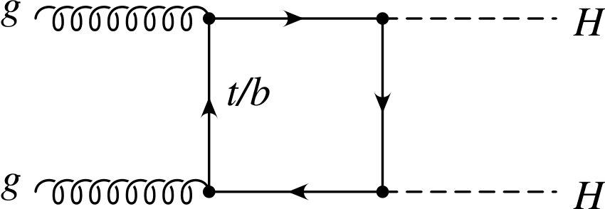 Figure 1
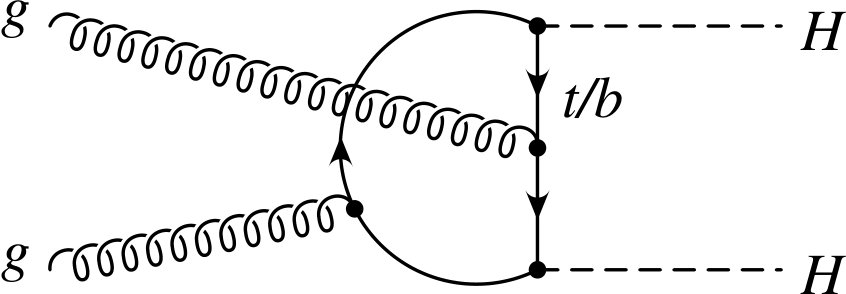 Figure 1
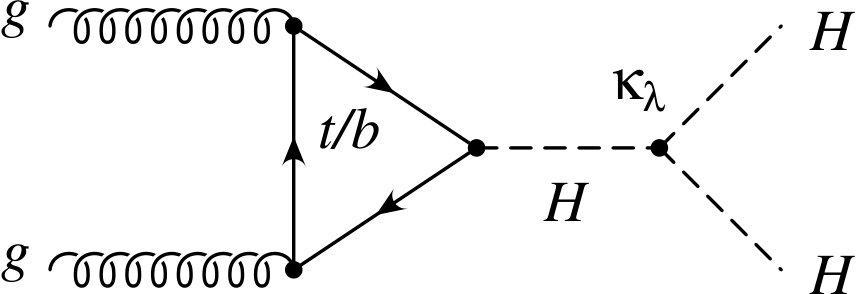 Figure 1
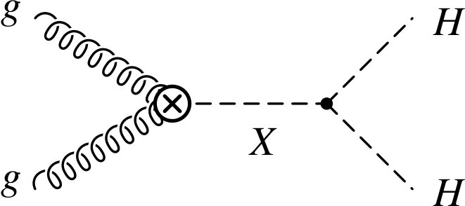 Figure 1
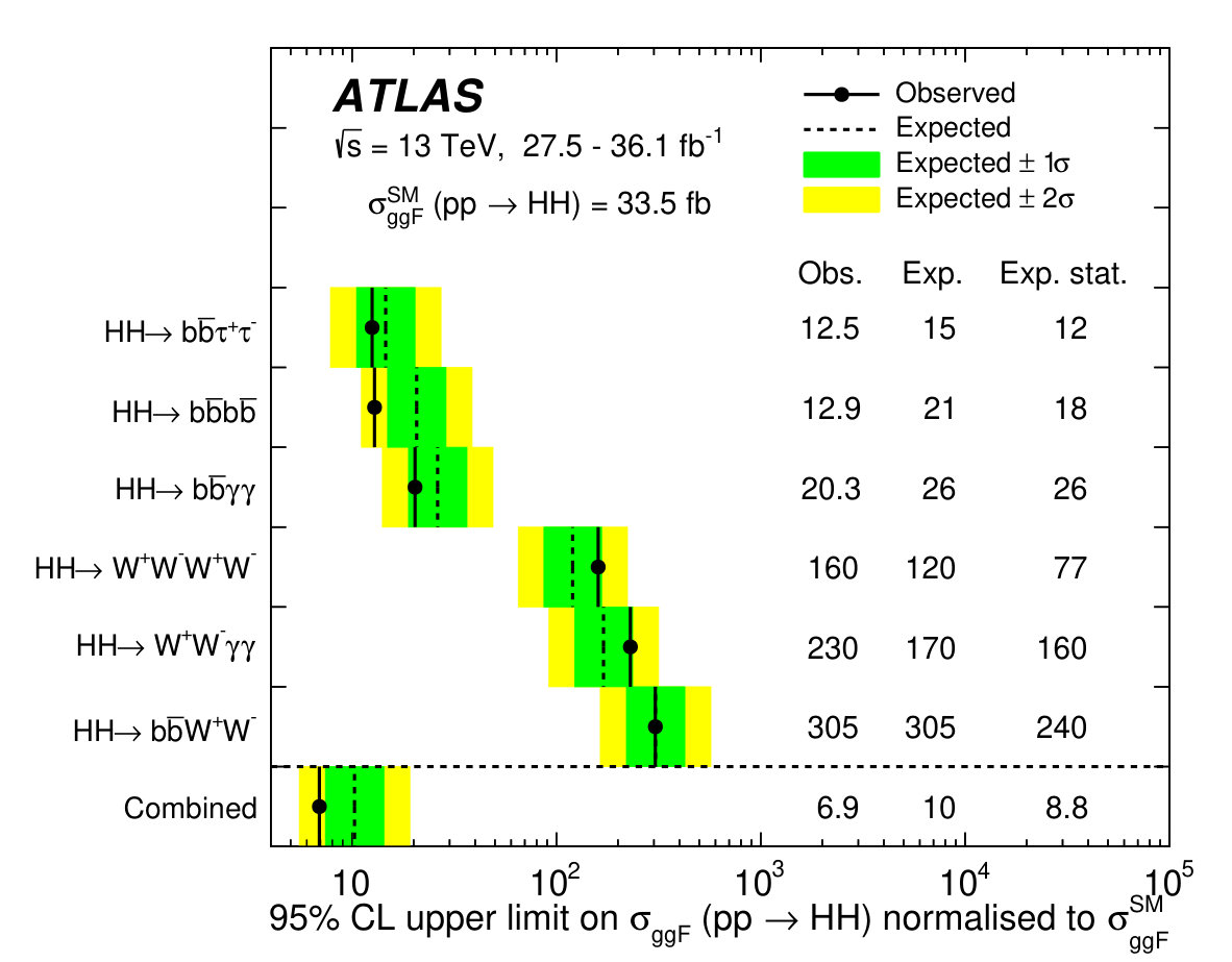 Figure 2
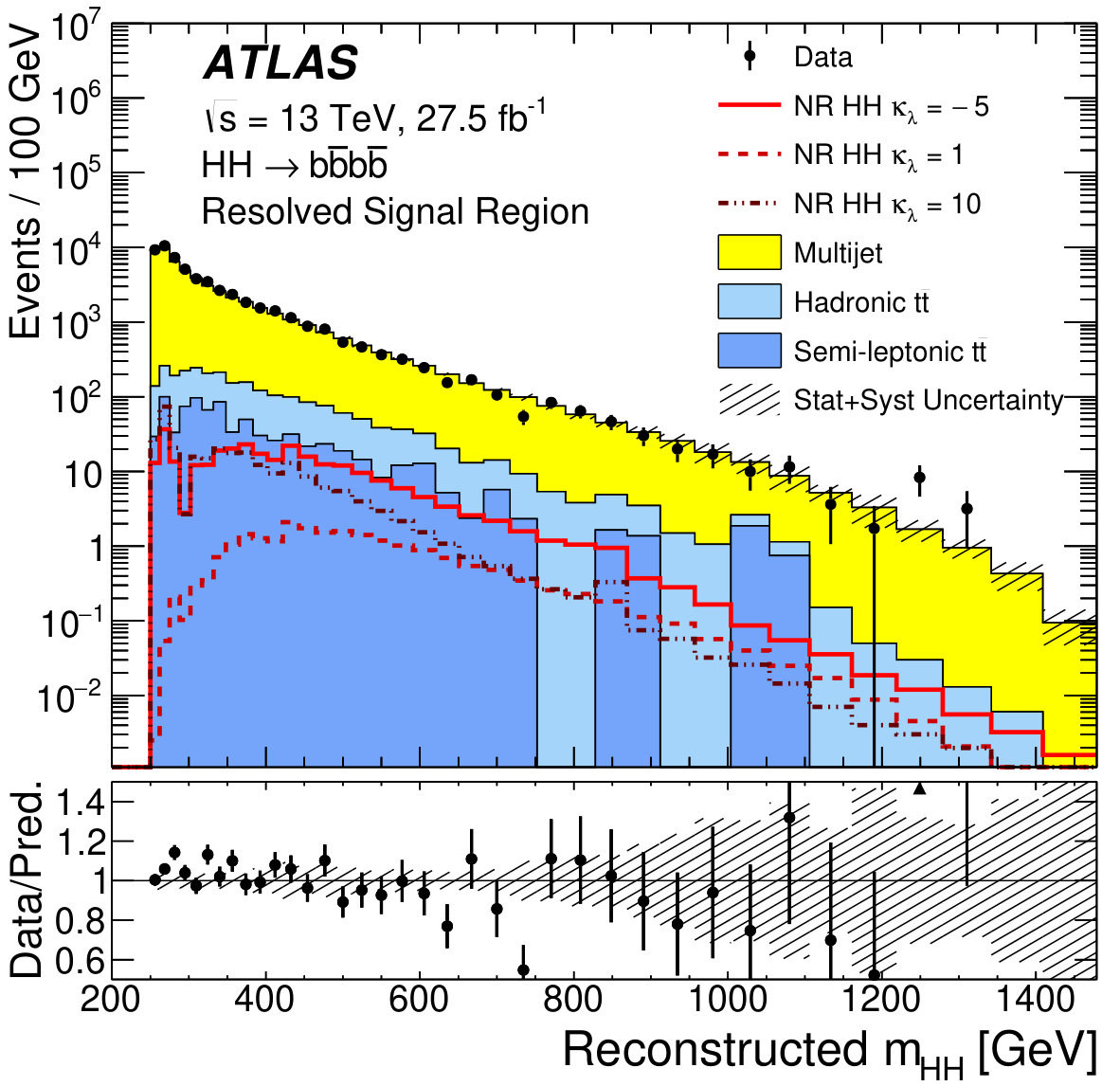 Figure 3
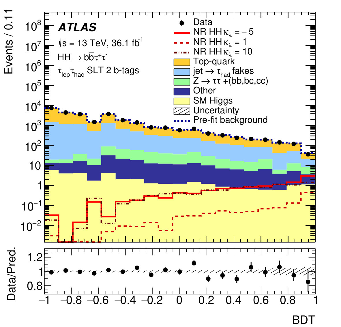 Figure 3
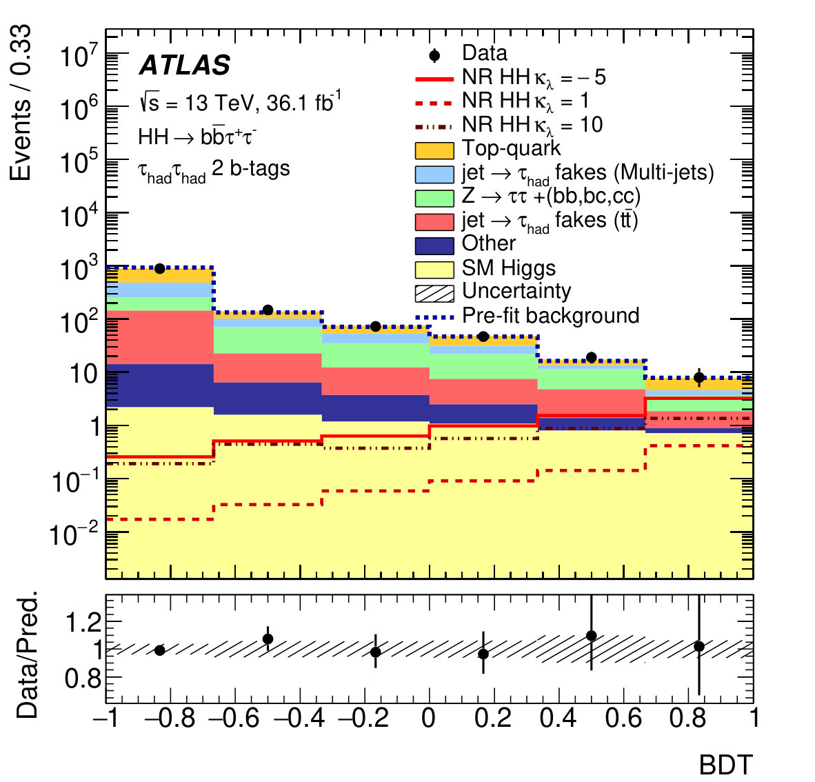 Figure 3
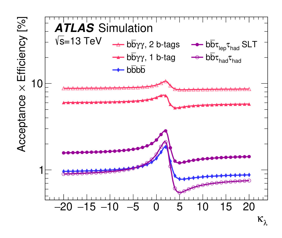 Figure 4
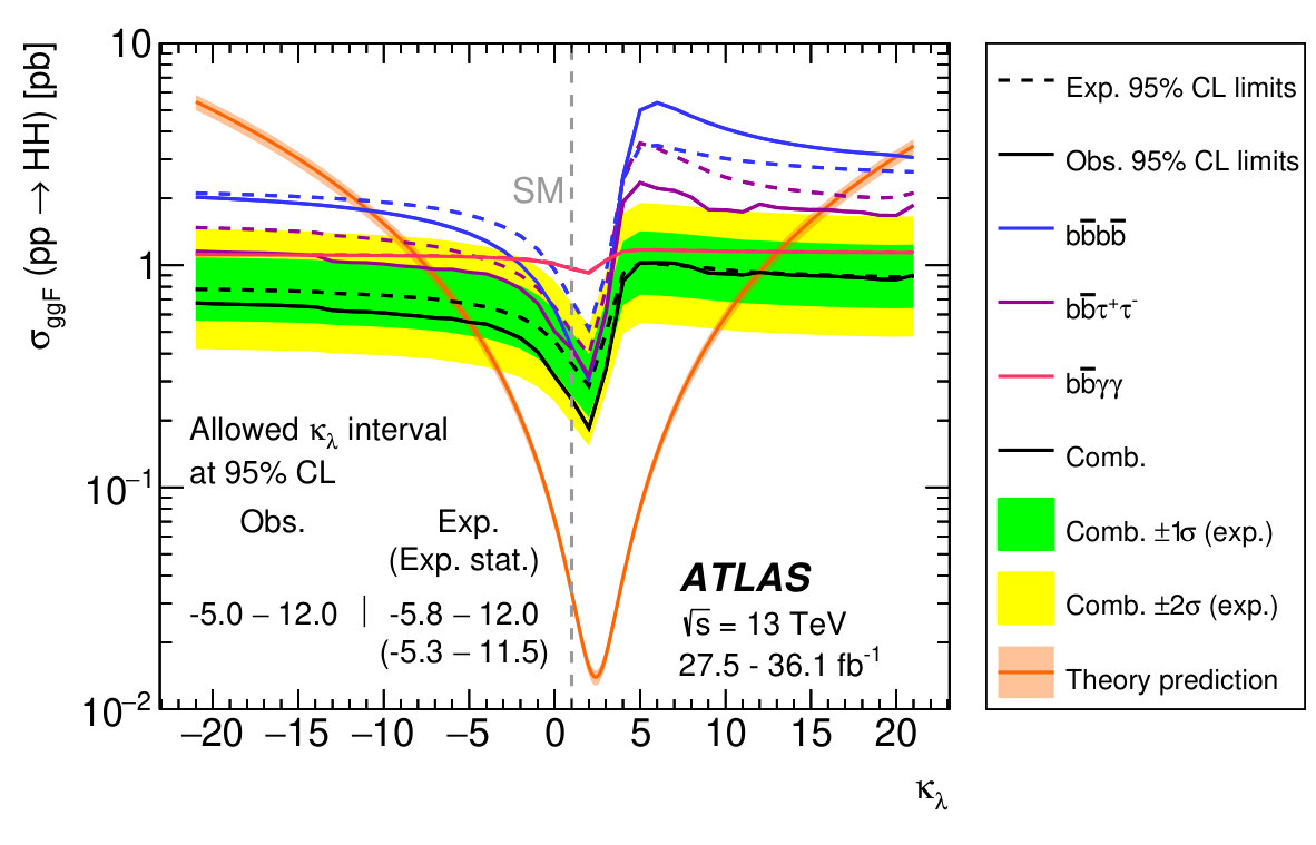 Figure 4
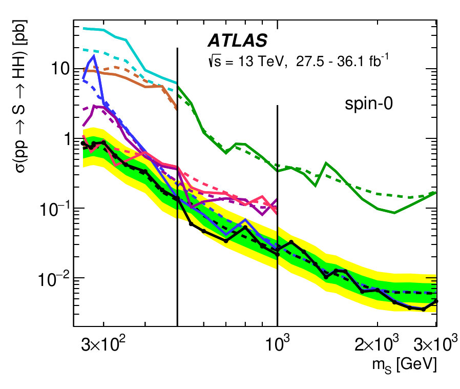 Figure 5
 Figure 5
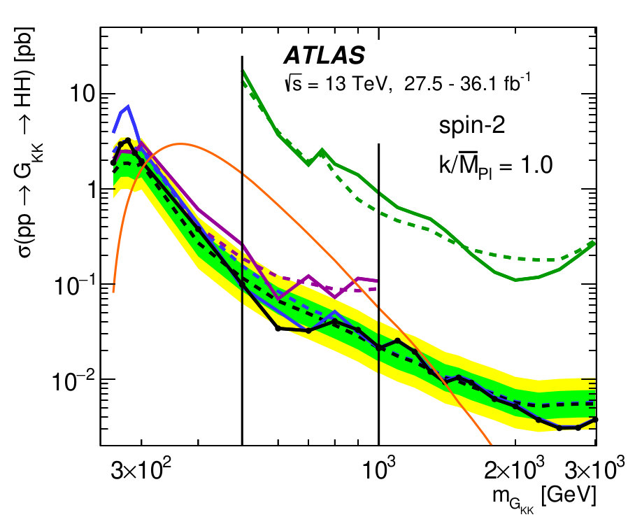 Figure 5
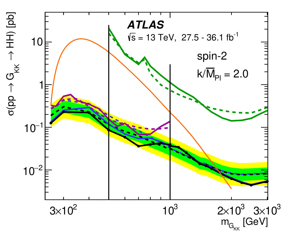 Figure 5
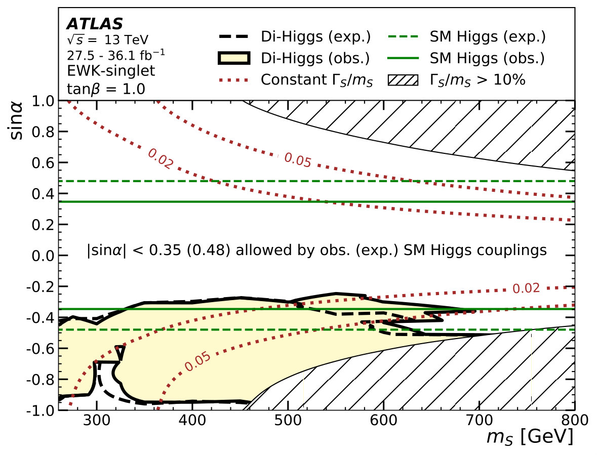 Figure 6
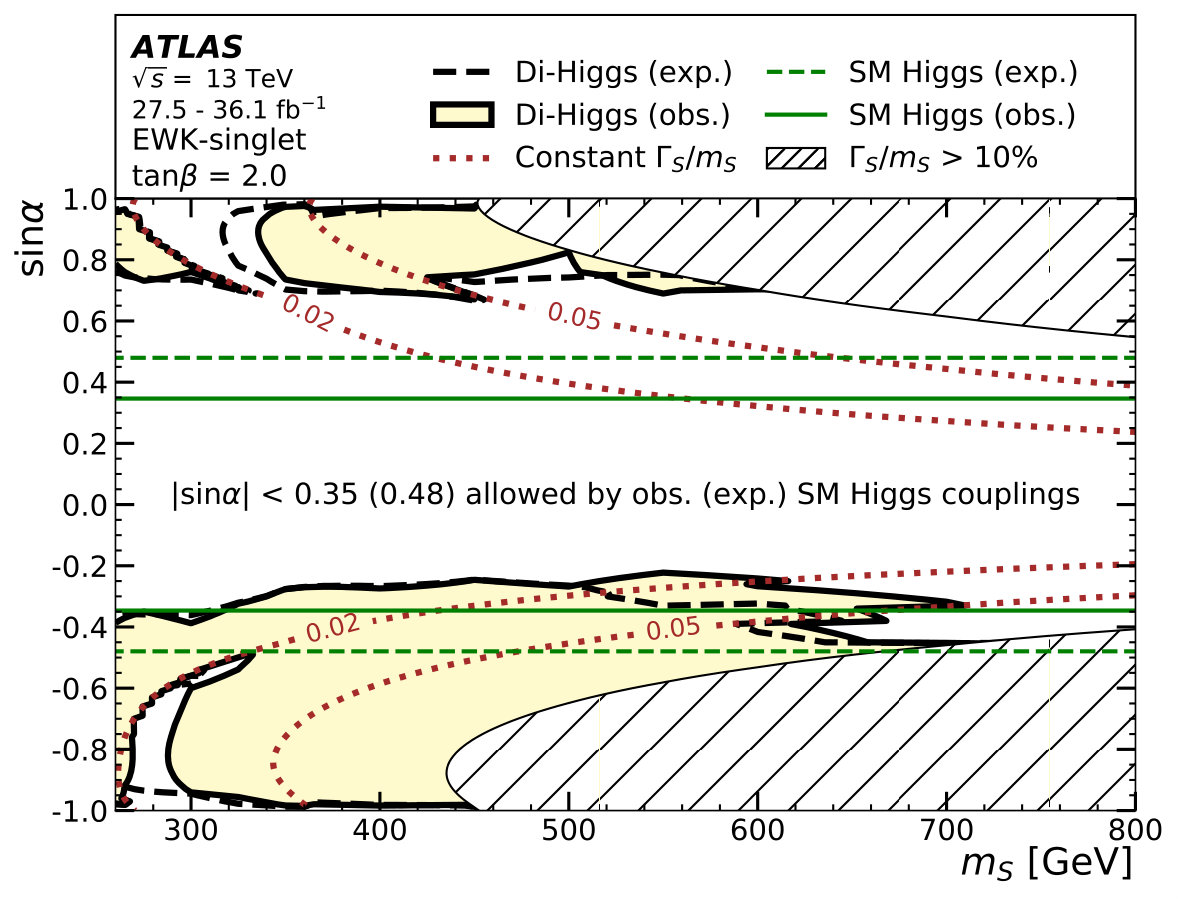 Figure 6
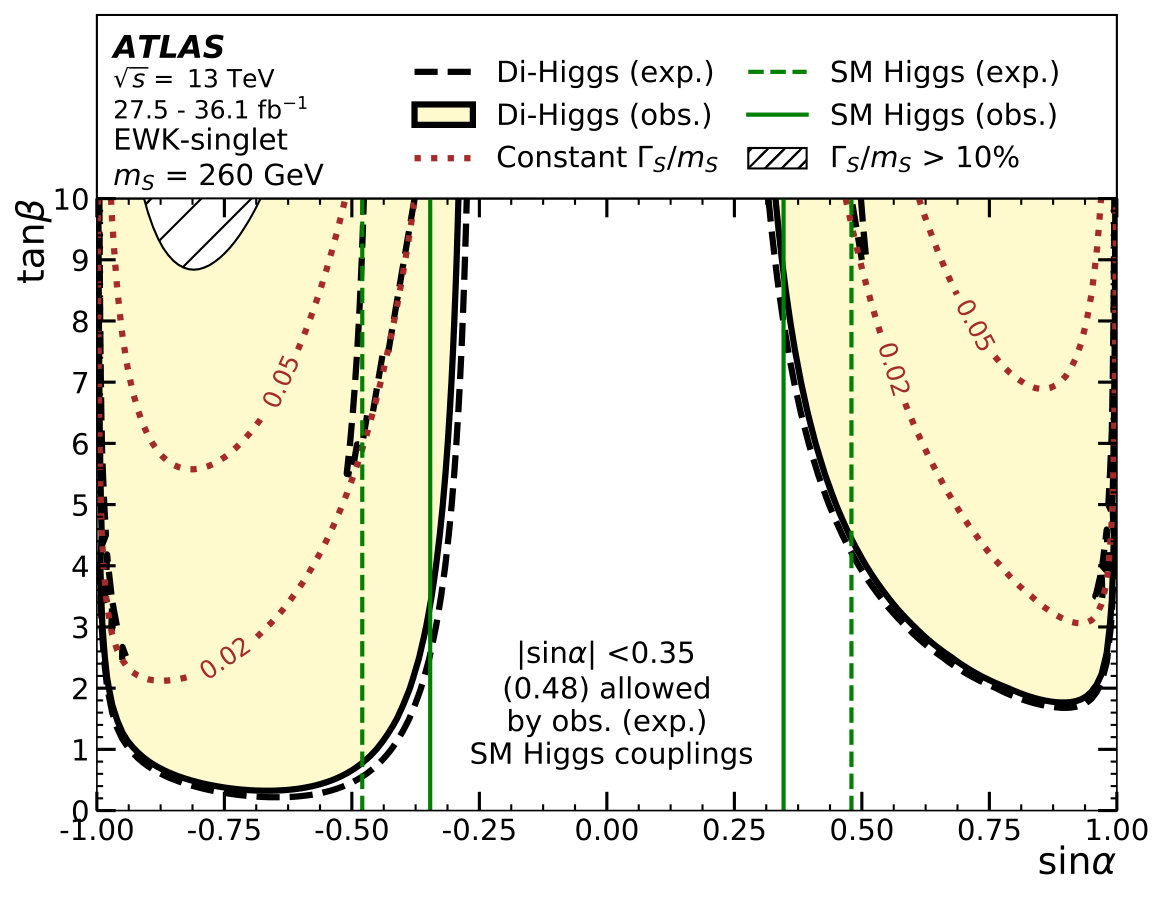 Figure 7
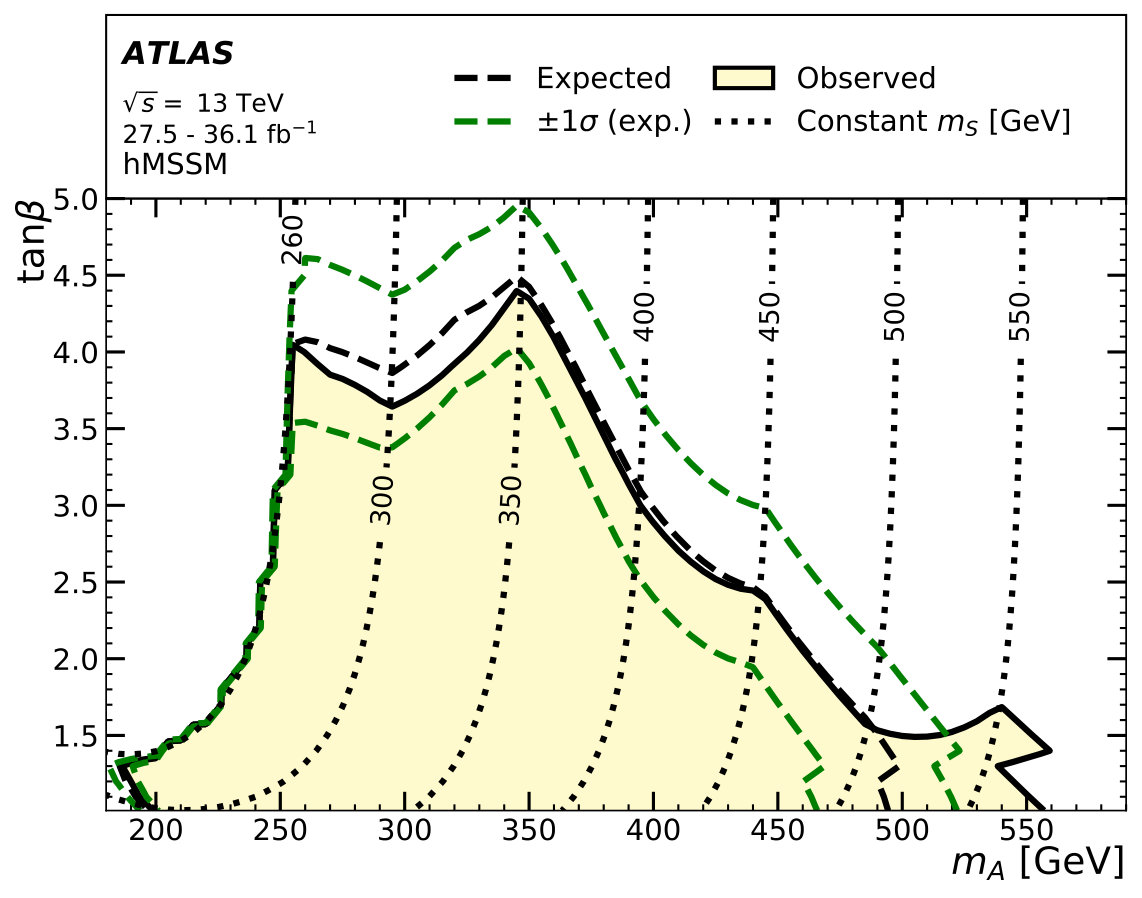 Figure 7
| 0.34 | 0.25 | 0.073 | 0.046 | |||
| [fb-1] | 27.5 [36.1] | 36.1 | 36.1 | 36.1 | 36.1 | 36.1 |
| Categories | 2 [2–5] | 1 [1] | 3 [2–3] | 9 [9] | 2 [2] | 1 [1] |
| Discriminant | [] | c.e. [] | BDT [BDT] | c.e. [c.e.] | [] | [] |
| Model | NR [] | NR [] | NR [] | NR [] | NR [] | NR [] |
| [TeV] | [0.26–3.00] | [0.50–3.00] | [0.26–1.00] | [0.26–0.50] | [0.26–1.00] | [0.26–0.50] |
| Ref. | [36] | [37] | [38] | [39] | [40] | [41] |
| Allowed interval at 95% CL | |||||||||
| Final state | Obs. | Exp. | Exp. stat. | ||||||
| — | — | — | |||||||
| — | — | — | |||||||
| — | — | — | |||||||
| Combination | — | — | — | ||||||
Peer Reviews
No public reviews on file for this paper yet. If you reviewed it on a platform where reviews are public (OpenReview, ICLR, NeurIPS, ICML), you can paste yours below so the community can read it here.
Videos
No videos yet. Explain this paper in a talk, walkthrough, or lecture? Add one.
\AtlasTitle
Combination of searches for Higgs boson pairs in collisions at 13 TeV with the ATLAS detector \AtlasAbstract This letter presents a combination of searches for Higgs boson pair production using up to 36.1 of proton–proton collision data at a centre-of-mass energy TeV recorded with the ATLAS detector at the LHC. The combination is performed using six analyses searching for Higgs boson pairs decaying into the , , , , and final states. Results are presented for non-resonant and resonant Higgs boson pair production modes. No statistically significant excess in data above the Standard Model predictions is found. The combined observed (expected) limit at 95% confidence level on the non-resonant Higgs boson pair production cross-section is () times the predicted Standard Model cross-section. Limits are also set on the ratio () of the Higgs boson self-coupling to its Standard Model value. This ratio is constrained at 95% confidence level in observation (expectation) to -4.97183$<\kappa_{\lambda}<$12.0122 (-5.81589$<\kappa_{\lambda}<$12.0083). In addition, limits are set on the production of narrow scalar resonances and spin-2 Kaluza–Klein Randall–Sundrum gravitons. Exclusion regions are also provided in the parameter space of the habemus Minimal Supersymmetric Standard Model and the Electroweak Singlet Model.
\AtlasRefCodeHDBS-2018-58 \AtlasJournalPhys. Lett. B \PreprintIdNumberCERN-EP-2019-099 \AtlasCoverSupportingNoteThe combination and interpretation of searches in collisions at TeV with the ATLAS detectorhttps://cds.cern.ch/record/2653800/ \AtlasCoverCommentsDeadline \AtlasCoverAnalysisTeam John Alison, Nansi Andari, Florian Beisiegel, Alessandra Betti, Petar Bokan, Elizabeth Brost, Patrick Bryant, Tyler Burch, Leo Cerda, David Delgove, Biagio Di Micco, Jochen Dingfelder, David Englert, Yaquan Fang, Arnaud Ferrari, Douglas Gingrich, Kathryn Grimm, Carl Gwilliam, Jonathan Hays, Tatjana Lenz, Qi Li, Gabriel Palacino, James Robinson, Nikolaos Rompotis, Eleonora Rossi, Jana Schaarschmidt, Chase Shimmin, Magdalena Slawinska, Xiaohu Sun, Alan Taylor, Tulin Varol, David Wardrope, Yu Zhang
\AtlasCoverEdBoardMemberKathrin Becker, John Hobbs, Jianming Qian (chair) \[email protected] \AtlasCoverEgroupEdBoardatlas-hdbs-2018-58-editorial-board@cern.ch \AtlasJournalRefPhys. Lett. B 800 (2020) 135103 \AtlasDOI10.1016/j.physletb.2019.135103
1 Introduction
The discovery of the Higgs boson () [1, 2] at the Large Hadron Collider (LHC) [3] in 2012 has experimentally confirmed the Brout–Englert–Higgs (BEH) mechanism of electroweak symmetry breaking and mass generation [4, 5, 6]. The BEH mechanism not only predicts the existence of a massive scalar particle, but also requires this scalar particle to couple to itself. Therefore, observing the production of Higgs boson pairs () and measuring the Higgs boson self-coupling is a crucial validation of the BEH mechanism. Any deviation from the Standard Model (SM) predictions would open a window to new physics. Moreover, the form of the Higgs field potential, which generates the Higgs boson self-coupling after electroweak symmetry breaking, can have important cosmological implications, involving, for example, predictions for vacuum stability or models in which the Higgs boson acts as the inflation field [7, 8, 9, 10].
In the SM, the gluon–gluon fusion process (ggF) accounts for more than 90% of the Higgs boson pair production cross-section, and only this production mode is considered here. It proceeds via two amplitudes: the first () represented by the diagrams (a) and (b), and the second () represented by the diagram (c) in Figure 1.
The interference between these two amplitudes is destructive and yields an overall cross-section of fb at TeV [11], calculated first at next-to-leading order (NLO) in QCD with the heavy top-quark approximation [12], then numerically with full top-quark mass dependence [13] (confirmed later in Ref. [14] and analytically computed with some approximation in Ref. [15]) corrected at next-to-next-to-leading order (NNLO) [16] in QCD matched with next-to-next-to-leading logarithmic (NNLL) resummation in the heavy top-quark limit [17, 18]. The Higgs boson mass used in these calculations and for all results in this paper is 125.09 GeV [19]. Beyond-the-Standard-Model (BSM) scenarios can bring substantial enhancement of this cross-section by modifying the relative sign of and , and by increasing . The amplitude is proportional to the Higgs self-coupling . The Higgs boson self-coupling modifier due to BSM scenarios is defined as . In this analysis, all other Higgs boson couplings are assumed to have SM values. Indirect limits on have been obtained using the measurements of single Higgs boson production and decay [20] and electroweak precision observables [21, 22], constraining to the range at 95% confidence level (CL). The Higgs boson self-coupling is discussed in the context of BSM models in Refs. [22, 23].
Several BSM models also predict the existence of heavy particles decaying into a pair of Higgs bosons. Two-Higgs-Doublet Models [24], models inspired by the Minimal Supersymmetric Standard Model (MSSM) like habemus MSSM (hMSSM) [25, 26, 27, 28], and Electroweak Singlet Models (EWK-singlet) [29, 30, 31, 11] predict, in addition to the Higgs boson, a second, heavier, CP-even scalar that can decay into two SM Higgs bosons. In the EWK-singlet model, the scalar states are mixed, with a mixing angle . The ratio of the vacuum expectation value of the additional singlet to that of the SM Higgs doublet, , is a free parameter. In the hMSSM, the CP-even states also mix, and the model’s phenomenology can be described by the mass () of a third, CP-odd, resonance and the ratio of the vacuum expectation values of the two Higgs doublets, . Alternatively, the Higgs boson pair can be produced resonantly through the decay of a spin-2 Kaluza–Klein (KK) graviton, as predicted in the Randall–Sundrum (RS) model of warped extra dimensions [32]. A schematic diagram for production of a heavy resonance followed by its decay into a Higgs boson pair is shown in Figure 1(d).
This letter presents a combination of results from searches for both non-resonant and resonant Higgs boson pair production in proton–proton () collisions at TeV. The data were collected with the ATLAS detector [33, 34, 35] and correspond to an integrated luminosity of up to 36.1 . The combination includes all published ATLAS search analyses using TeV data, namely those studying the final states [36], [37], [38], [39], [40] and [41].
Previous combinations of searches for pair production were performed at TeV by the ATLAS experiment [42] and at TeV by the CMS experiment [43] combining the final states [44, 45, 46, 47], VV [48], [49] and [50].
2 Analysis description
The analysis strategies for each of the final states considered in this letter are summarised below.
- •
The analysis is performed using four anti- jets reconstructed with a radius parameter [51, 52] (resolved analysis) or two large- jets with (boosted analysis). The dataset of the resolved analysis is split according to the years 2015 and 2016, and then statistically combined taking into account the different trigger algorithms used in 2015 and 2016. In part of the 2016 data period, inefficiencies in the online vertex reconstruction affected -jet triggers that were used in the resolved analysis, reducing the total available integrated luminosity to 27.5 fb*-1*. The boosted analysis searches for two large- jets containing the -quark pairs from the decays of the two Higgs bosons. The large- jets are identified as originating from -quarks using a -tagging algorithm applied to track-jets [53] associated with the large- jet [54]. The analysis is divided into three categories: the first category selects events in which each of the two large- jets has one -tagged track-jet; the second category requires that one large- jet contains two -tagged track-jets and the other large- jet contains one -tagged track-jet; the third category requires that both large- jets contain two -tagged track-jets. For the SM search, only the resolved analysis is used, with two categories, one for the 2015 and another for the 2016 dataset. The resonant search is instead performed with the resolved analysis for masses in the range 260–1400 GeV, with the boosted analysis for masses in the range 800–3000 GeV, and with the combination of the two for masses in the overlapping range 800–1400 GeV.
- •
The analysis looks for the decay channel, where is an electron or muon, and is a quark or anti-quark. The pair is selected from two jets (resolved analysis) or one large- jet (boosted analysis), while the jets from the decay are reconstructed with jets. The resolved analysis is used in the SM search, in the search for a scalar resonance with a mass between 500 and 1400 GeV, and in the search for a KK graviton in the mass range 500 to 800 GeV. The boosted analysis looks for scalar resonances in the mass range 1400 to 3000 GeV and for KK gravitons between 800 and 3000 GeV. The resolved and boosted analyses each use one category. The two analyses are not statistically combined due to a significant overlap between the two signal regions.
- •
The analysis looks for final states with two -tagged jets and two -leptons. One of the two -leptons of the pair is required to decay hadronically, while the other decays either hadronically () or leptonically (). In the channel, events are triggered by single lepton triggers (SLT), requiring an electron or a muon in the final state, or by the coincidence of a lepton trigger with a hadronic trigger (LTT). In the channel, events are triggered by single hadronic triggers (STT) or double hadronic triggers (DTT). The analysis is divided into three categories: one selects events, a second selects events triggered by the SLT, and a third selects events triggered by the LTT. The and the SLT categories are used for all model interpretations, while the LTT category is used in the SM search (excluding the analysis) and in resonant searches up to a mass of 800 GeV.
- •
The analysis looks for channels with leptonic and/or hadronic decays. Three channels are identified: , , and , with being an electron or muon, a quark, and a neutrino. The momentum is reconstructed from jets. In order to suppress jets and background, dilepton events are required to have two leptons of the same charge. Events are categorised according to the lepton flavour (, and ). Three-lepton events are selected if the sum of the lepton charges is 1. They are divided into two categories according to the number of same-flavour, opposite-charge (SFOS) lepton pairs; one category selects zero SFOS lepton pairs and a second category selects one or two SFOS lepton pairs. Four-lepton events are categorised according to the number of SFOS lepton pairs and the invariant mass () of the four-lepton system. Four categories are defined, requiring that the number of SFOS lepton pairs is less than two or equal to two, and is smaller or larger than 180 GeV. A total of nine categories are fit simultaneously in the searches for both non-resonant and resonant production.
- •
The analysis searches for a pair decaying into and . Two high- isolated photons are required to have 0.35 and 0.25 respectively. The events are then analysed using two selections: a ‘loose selection’ requiring a jet with GeV and a second jet with GeV, and a ‘tight selection’ where the two jets are required to have larger than 100 and 30 GeV. All jets have a radius parameter . Both selections are subdivided into two categories requiring one -tagged jet or two -tagged jets. The tight selection is used in the SM search and in the search for resonances with masses higher than 500 GeV, while the loose selection is used in the analysis and in the search for resonances with masses smaller than 500 GeV. The analysis is therefore divided into four categories, but only two of them are simultaneously fit to extract each result.
- •
The analysis searches for a pair decaying into and . The analysis uses the same photon selection as the channel and looks for one decaying leptonically and a second decaying hadronically (). The hadronic decay is reconstructed from jets. Only one category is used in the searches for both non-resonant and resonant production.
A summary of the main analysis characteristics is given in Table 1. All analyses impose a series of sequential requirements on kinematic variables to select signal events and suppress backgrounds. The analysis uses a boosted decision tree (BDT) [55] distribution as the final discriminant for both the non-resonant and resonant searches. For the resonant searches, the , and analyses use the invariant mass () as the final discriminant, the analysis uses the invariant mass (), while uses simple event counting. For the SM search, the analysis uses the distribution as a discriminant, profiting from the difference between the shapes of the signal and the dominant multi-jet background. The and analyses fit the distribution to extract both the signal yield and the background expectation, while the and analyses use event counting.
3 Statistical treatment
The statistical interpretation of the combined search results is based on a simultaneous fit to the data for the cross-section of the signal process and nuisance parameters that encode statistical and systematic uncertainties, using the CLS approach [56]. The asymptotic approximation [57] is used in the analysis of all final states and their combination.
All signal regions considered in the simultaneous fit are either orthogonal by construction or have negligible overlap. The overlap due to object misidentification between and , and between and , which are not orthogonal by construction, is evaluated by running the signal and data samples from each channel through the analysis selection of each other channel. Less than 0.1% of simulated signal events overlap between analyses, and no overlap is found in data. There is some irreducible contamination from and events with ’s in the final state passing the selection. This contamination is less than 8% of the selected events, and it is not taken into account in the analysis, note that including this contribution would increase the analysis sensitivity therefore the results obtained here are slightly conservative. The detector systematic uncertainties, such as those in jet reconstruction, -jet tagging, electron, muon and photon reconstruction and identification, as well as the uncertainty on the integrated luminosity [58], are correlated across all final states. Uncertainties on the signal acceptance derived by varying the renormalisation and factorisation scales, the parton distribution functions and the parton shower are correlated too. Theoretical and modelling systematic uncertainties of the backgrounds derived using simulated events are not correlated across different analyses because the overlap among their contributions to the different analyses is negligible.
4 Combination of results on non-resonant Higgs boson pair production
The SM analyses use signal samples generated at next-to-leading order (NLO) in QCD with Madgraph5_aMC@NLO [59] using the CT10 NLO parton distribution function (PDF) set [60]. Parton showers and hadronisation were simulated with Herwig++ [61] using parameter values from the UE-EE-5-CTEQ6L1 tune [62]. The so-called FTApprox method [63] is applied in the event generation to include finite top-quark mass effects in the real-radiation NLO corrections. The virtual-loop corrections are realised with Higgs effective field theory (HEFT) assuming infinite top-quark mass. The generated events are then corrected with a generator level bin-by-bin reweighting of the distribution, which is calculated with finite top-quark mass in full NLO corrections [13]. The branching fractions of the Higgs boson are assumed to be equal to the SM predictions [11]. For the SM search, upper limits are extracted for the cross-section of production and are normalised by the SM cross-section . The limits are determined assuming that all kinematic properties of the pair are those predicted by the SM, particularly the distribution, and only the total ggF production cross-section, , is allowed to deviate from its SM value. The theoretical uncertainties of are less than 10% [11] and are not included in the fit results.
The upper limits at 95% CL on the cross-section of the ggF Higgs boson pair production normalised to are shown in Figure 2 for the individual final states and their combination. The upper limit for each final state is obtained from a fit with minimal changes from previously published results. The changes include an update of the ggF Higgs boson pair production cross-section from 33.4 fb to 33.5 fb for all final states. Additionally, the final state included theoretical uncertainties on the ggF inclusive cross-section, , which are not considered in the present treatment, and the final state is updated to use an asymptotic approximation to calculate the observed limit instead of the pseudo-experiment method used for its publication. This results in a 10% change in the observed limit of . Moreover, the impact of the asymptotic approximation on all final states combined is found to be 5%.
The combined observed (expected) upper limit on the SM production is () . The expected limit is similar to the CMS result of 12.8 . The observed limit is more stringent for the ATLAS result than the CMS result of 22.2 because the three leading channels (, and ) have a data deficit in ATLAS and an excess in CMS [43], remaining however within the two 2 uncertainty interval. Detailed comparisons can be found in Ref. [64].
The impact of the systematic uncertainties has been evaluated by recomputing the limit without their inclusion. The limit is then reduced by 13% when removing all of them. The main sources of systematic uncertainty are the modelling of the backgrounds, the statistical uncertainty of simulated events and the -lepton reconstruction and identification. When removed the limit reduces by 5%, 3% and 2%, respectively.
5 Constraints on the Higgs boson self-coupling
The results in Figure 2 show that the sensitivity of the SM search is driven by the final states , and . These final states are used to set constraints on the Higgs boson self-coupling modifier . After setting all couplings to fermions and bosons to their SM values, a scan of the self-coupling modifier is performed. The factor affects both the production cross-section and the kinematic distributions of the Higgs boson pairs, by modifying the production amplitude. It can also affect the Higgs boson branching fractions due to NLO electroweak corrections [20], but this dependence is neglected in the following.
The signal used in the fit was simulated according to the following procedure. For each value of the spectrum is computed at the generator-level, using the leading-order (LO) version of MadGraph5_aMC@NLO [59] with the NNPDF 2.3 LO [65] PDF set, together with Pythia 8.2 [66] for the showering model using the A14 tune [67]. Because only one amplitude of Higgs boson pair production depends on , linear combinations of three LO samples generated with different values of are sufficient to make predictions for any value of . Binned ratios of the distributions to the SM distribution are computed for all values and then used to reweight the events of NLO SM signal samples, generated using the full detector simulation. This procedure is validated by comparing kinematic distributions obtained with the reweighting procedure applied to the LO SM sample and LO samples generated with the actual values set in the event generator. The two sets of distributions are found to be in agreement. This procedure assumes that higher order QCD corrections on the differential cross-section as a function of are independent of . The reweighted NLO signal sample is used to compute the signal acceptance and the kinematic distributions for different values of .
This letter presents results for the first time in the ATLAS and final states and incorporates the previously published result for the final state. The analyses closely follow the SM search, with some exceptions which are discussed below for each final state.
- •
In the final state, the same analysis selection and final discriminant are used in the -scan analysis and in the SM search. The distribution of the final discriminant is shown in Figure 3(a), where, with the exception of a small excess in the region below 300 GeV [36] and a small deficit in the 500-600 GeVregion, good agreement between data and the expected background is observed. The shape of the distribution has a strong dependence on , and the signal acceptance varies by a factor 2.5 over the probed range of -values () shown in Figure 4(a). The two effects together determine how the exclusion limits on the cross-section of the production vary as a function of .
- •
In the final state, as in the SM search, both and events are used. In contrast with the SM search, LTT events (see Section 2) are not used given their negligible contribution. The SM search and the -scan analysis use the same sets of variables to build BDT discriminants. For the -scan the BDTs are retrained using the NLO SM signal sample reweighted with , ensuring good sensitivity over the whole range of probed -values. The BDT score distributions are used in the fit to compute the final results. The shape of the BDT distributions does not show a dependence as strong as in the final state, as can be seen in Figure 3. The sensitivity of this analysis is instead affected by a variation in the signal acceptance by up to a factor of three over the probed range of -values, as shown in Figure 4(a).
- •
In the final state, the loose selection is used in the -scan analysis because the average transverse momentum of the Higgs bosons is lower at large values of , where dominates the production cross-section. As in the SM search, the statistical analysis is performed using the distribution, which does not depend on . The signal acceptance varies by about 30% over the probed range of -values, as shown in Figure 4(a). In the previously published analysis [40], LO samples were used for the computation of the signal acceptance, while in this paper the NLO reweighted samples are used, as described above.
\floatsetup
[figure]style=plain,subcapbesideposition=center
The signal acceptance times efficiency as a function of is shown in Figure 4(a). Given that, for each final state, the same selection was applied over the full scanned range, the shape of the acceptance times efficiency curve is determined by the variation of the event kinematics as a function of . For high values of the term dominates the total amplitude, causing a softer spectrum, and thus a lower acceptance times efficiency. Around = 2.4 the interference between and amplitudes is maximal, producing the hardest spectrum and, consequently, the highest signal acceptance times efficiency.
In each analysis, and in their combination, the 95% CL upper limit on the cross-section is computed for different values of . The results are shown in Figure 4(b). The theoretical cross-section as a function of is overlaid in the figure. It is computed by multiplying the SM cross-section by the ratio of the cross-section computed at , to the same quantity computed at . The factor is computed at NNLO+NNLL with the infinite top-quark mass approximation [68]. The resulting observed (expected) confidence interval at 95% CL for is: ( ) .
In Figure 4(b) the shape of the upper-limit curves approximately follows the inverse of the signal acceptance shown in Figure 4(a). In the analysis, the observed limits are more stringent than the expected limits at low values of . For these values the signal distributions have significant populations in the region 500-600 GeV, where the data deficit sits, as explained above. For larger values of the distribution is shifted to lower values, and thus the excess in data below 300 GeV leads to the observed limits being less stringent than expected. In the final state the observed limits are more stringent than the expected limits over the whole range of , due to a deficit of data relative to the background predictions at high values of the BDT score. The limit shows a weaker dependence on than the and limits because the acceptance varies less as function of .
The 95% CL allowed intervals are given in Table 2. The systematic uncertainties weaken the limits by less than 10% relative to those obtained with only statistical uncertainties. The final state least (most) affected by systematic uncertainties is (). The Higgs boson branching fraction depends on due to NLO electroweak corrections [20]. This dependence is neglected in the present treatment, but its overall impact on the allowed interval is evaluated to be no more than 7%. Theory uncertainties on the signal cross section shown in Fgure 4(b) are not taken into account when computing the limits in Table 2, they affect the limit by less than 8%.
6 Combination of results for resonant Higgs boson pair production
The resonance decaying into a pair of Higgs bosons is assumed to be either a heavy spin-0 scalar particle, , with a narrow width or a spin-2 KK graviton, .
The search for the heavy scalar particle is performed with all six final states included in this combination. With the exception of and , all signal samples were simulated at NLO with MadGraph5_aMC@NLO using the CT10 PDF set. The matrix-element generator was interfaced to Herwig++ with the UE-EE-5-CTEQ6L1 tune. The final state uses an LO model generated with MadGraph5_aMC@NLO using the NNPDF 2.3 LO PDF set interfaced to Pythia 8.2 with the A14 tune, while the final state uses the same LO event generator but interfaced to Herwig++ with the UE-EE-5-CTEQ6L1 tune.
The scalar resonance search is performed in the mass range 260–3000 GeV, and within this range no statistically significant excess is observed. In the combination, the largest observed deviation from the background expectation is 1 for the search mass range. The combined upper limit on the cross-section is shown as a function of the resonance mass in Figure 5(a). Systematic uncertainties have a sizeable effect on the upper limits depending on the probed resonance mass. The total impact of systematics or the impact of a single systematic uncertainty has been evaluated by computing the percentage reduction of the upper limit obtained by removing all systematic uncertainties or a particular source. Overall the systematic uncertaintes affect the limit by 12% (11%) for a resonance mass of 1 (3) TeV. Among them, the largest systematic uncertainties are due to the modelling of the backgrounds, impacting the upper limit by 7% (9%) at 1 (3) TeV. The second leading systematic uncertainty comes from -tagging, that affects the upper limit by 2% at 1 TeV, but its impact is negligible at 3 TeV where relative background and statistical uncertainties increase significantly. At 3 TeV the second leading systematic uncertainty is related to the jet energy scale and resolution, changing the limit by 2%. Interpretations in specific spin-0 BSM models are provided in Section 7.
The search for a spin-2 KK graviton is performed with the , and final states only. Gravitons were simulated using an LO model in MadGraph5_aMC@NLO with the NNPDF 2.3 LO PDF set interfaced to Pythia 8.2 with the A14 tune. The resonance width changes with the graviton mass and depends on the parameter , where is the curvature of the warped extra dimension in the bulk RS model and is the effective four-dimensional Planck mass. The search is performed for models with equal to 1 and 2. For = 1 (2), the width ranges from 3% (11%) for a 0.3 TeV graviton mass to 6% (25%) for a 3 TeV graviton mass.
The upper limits in the search are shown as a function of the resonance mass in Figures 5(b) and 5(c) for equal to 1 and 2, respectively. In the combination, the largest observed deviation from the background expectation is 1.5 (0.7) for the search mass range with 1 (2). Exclusion ranges on the graviton mass are obtained by comparing the upper limit with the production cross section calculated at LO. In the case of , the bulk RS model is excluded at 95% CL in the graviton mass range from GeV to GeV. In the case of , the model is excluded at 95% CL for graviton masses from 260 GeV, where the scan starts, to GeV.
The impact of the systematic uncertainties on the upper limits on has a small dependence on the resonance mass. It is 20% over the whole mass range for , and 29% (25%) at a mass of 1 TeV (3 TeV) for . The largest systematic uncertainties are from the modelling of the backgrounds, affecting the limit by 11% (15%) at 1 TeV (3 TeV) for and 16% (21%) at 1 TeV (3 TeV) for . For , the subleading systematic uncertainties come from -tagging at low mass, that affect the limit by 3%, and from jet energy scale and resolution at high mass, that affect the upper limit by 2% (3%) at 1 TeV (3 TeV). For , subleading systematic uncertainties are from jet energy scale and resolution, impacting the upper limits by 5% at 1 TeV and 4% at 3 TeV. The systematic uncertainties affect upper limits more for than for , because the natural width of the signal graviton is four times larger with .
7 Constraints on the hMSSM and EWK-singlet models
Exclusion limits are also presented for two specific models, namely the EWK-singlet model [29, 30, 31, 11] and the hMSSM model [26, 69, 27, 28, 11]. The sensitivity of the , and final states to these models is negligible, so the presented results combine only the , and final states.
For the EWK-singlet model, the experimental limits on the spin-0 resonance (as reported in Section 6) are interpreted as constraints in the – plane (where is the resonance mass) for and , shown in Figure 6(a) and Figure 6(b) respectively. The expected cross-section for each point in the parameter space is obtained by scaling the heavy Higgs cross-section calculated at NNLO+NNLL [11] with singlet coupling modifiers. The branching fractions are computed with sHDECAY [70]. In this model, the width of the heavy scalar can be large in some regions of the parameter space. Due to the use of narrow-width signal models in the event generation, results presented here are valid only in regions of the model parameter-space where the resonance width () is smaller than the experimental resolution at the resonance mass. This holds when % for , % for and % for . Therefore, the excluded region in the plot is obtained by combining the three final states for %, by combining the and final states for 2% %, and using only for 5% %. The hatched region shows points where %, where no exclusion can be provided. Figure 7(a) shows limits for the (sin , tan ) parameter space for GeV where, due to the limited decay phase space, the resonance width is narrow in a wide region of the parameter space.
The experimental limits on a spin-0 resonance are also interpreted as constraints in the – plane of the hMSSM model in Figure 7(b). The expected cross-section for each point in the parameter space is obtained using the gluon-gluon fusion cross-section from SUSHI 1.5.0 [71, 72] and the branching fractions computed with HDECAY 6.4.2 [73].
The excluded region is more than doubled along relative to the previous combined results in Ref. [42] at 8 TeV, and excludes values of from 190 GeV to 560 GeV depending on . The kink at low and high values is caused by removing the final state from the combination in the region where the predicted width of the heavy CP-even Higgs boson is larger than the experimental resolution on in the analysis.
8 Conclusion
A statistical combination of six final states , , , , and , is presented for the search for non-resonant and resonant production of Higgs boson pairs. These searches use up to 36.1 of proton–proton collision data at 13 TeV recorded with the ATLAS detector at the LHC111All results are available in digital format on HEPDATA at the following link: https://www.hepdata.net/record/90521.
In both resonant and non-resonant searches, no statistically significant excess of events above the Standard Model predictions is found. For the Standard Model production mode, the observed (expected) 95% confidence level upper limit on the gluon–gluon fusion cross-section is () times the Standard Model prediction. The expected limit is comparable to the CMS result, while the observed limit is significantly stronger than CMS’s due to a data deficit compared to expected background in ATLAS and an excess in CMS. For the resonant case, upper limits are set on the production cross-section of heavy spin-0 and spin-2 resonances decaying into pairs of Higgs bosons in the mass range 260–3000 GeV.
Upper limits on the cross-section are also computed as a function of the Higgs boson self-coupling modifier , by combining the , and final states. The combination excludes values outside the range -4.97183$<\kappa_{\lambda}<$12.0122 (-5.81589$<\kappa_{\lambda}<$12.0083) at 95% confidence level in observation (expectation). The three final states are also combined to constrain the Electroweak Singlet Model in the (, sin ) and the (sin , tan ) parameter spaces and the habemus Minimal Supersymmetric Standard Model in the (, tan ) parameter space.
Acknowledgements
We thank CERN for the very successful operation of the LHC, as well as the support staff from our institutions without whom ATLAS could not be operated efficiently.
We acknowledge the support of ANPCyT, Argentina; YerPhI, Armenia; ARC, Australia; BMWFW and FWF, Austria; ANAS, Azerbaijan; SSTC, Belarus; CNPq and FAPESP, Brazil; NSERC, NRC and CFI, Canada; CERN; CONICYT, Chile; CAS, MOST and NSFC, China; COLCIENCIAS, Colombia; MSMT CR, MPO CR and VSC CR, Czech Republic; DNRF and DNSRC, Denmark; IN2P3-CNRS, CEA-DRF/IRFU, France; SRNSFG, Georgia; BMBF, HGF, and MPG, Germany; GSRT, Greece; RGC, Hong Kong SAR, China; ISF and Benoziyo Center, Israel; INFN, Italy; MEXT and JSPS, Japan; CNRST, Morocco; NWO, Netherlands; RCN, Norway; MNiSW and NCN, Poland; FCT, Portugal; MNE/IFA, Romania; MES of Russia and NRC KI, Russian Federation; JINR; MESTD, Serbia; MSSR, Slovakia; ARRS and MIZŠ, Slovenia; DST/NRF, South Africa; MINECO, Spain; SRC and Wallenberg Foundation, Sweden; SERI, SNSF and Cantons of Bern and Geneva, Switzerland; MOST, Taiwan; TAEK, Turkey; STFC, United Kingdom; DOE and NSF, United States of America. In addition, individual groups and members have received support from BCKDF, CANARIE, CRC and Compute Canada, Canada; COST, ERC, ERDF, Horizon 2020, and Marie Skłodowska-Curie Actions, European Union; Investissements d’ Avenir Labex and Idex, ANR, France; DFG and AvH Foundation, Germany; Herakleitos, Thales and Aristeia programmes co-financed by EU-ESF and the Greek NSRF, Greece; BSF-NSF and GIF, Israel; CERCA Programme Generalitat de Catalunya, Spain; The Royal Society and Leverhulme Trust, United Kingdom.
The crucial computing support from all WLCG partners is acknowledged gratefully, in particular from CERN, the ATLAS Tier-1 facilities at TRIUMF (Canada), NDGF (Denmark, Norway, Sweden), CC-IN2P3 (France), KIT/GridKA (Germany), INFN-CNAF (Italy), NL-T1 (Netherlands), PIC (Spain), ASGC (Taiwan), RAL (UK) and BNL (USA), the Tier-2 facilities worldwide and large non-WLCG resource providers. Major contributors of computing resources are listed in Ref. [75].
The reference list from the paper itself. Each links out to its DOI / PubMed record.
- 1[1] ATLAS Collaboration “Observation of a new particle in the search for the Standard Model Higgs boson with the ATLAS detector at the LHC” In Phys. Lett. B 716 , 2012, pp. 1–29 DOI: 10.1016/j.physletb.2012.08.020 · doi ↗
- 2[2] CMS Collaboration “Observation of a new boson at a mass of 125 Ge V with the CMS experiment at the LHC” In Phys. Lett. B 716 , 2012, pp. 30–61 DOI: 10.1016/j.physletb.2012.08.021 · doi ↗
- 3[3] L. Evans and P. Bryant “LHC Machine” In J. Instrum. 3 , 2008, pp. S 08001 DOI: 10.1088/1748-0221/3/08/S 08001 · doi ↗
- 4[4] F. Englert and R. Brout “Broken Symmetry and the Mass of Gauge Vector Mesons” In Phys. Rev. Lett. 13 , 1964, pp. 321–323 DOI: 10.1103/Phys Rev Lett.13.321 · doi ↗
- 5[5] Peter W. Higgs “Broken Symmetries and the Masses of Gauge Bosons” In Phys. Rev. Lett. 13 , 1964, pp. 508–509 DOI: 10.1103/Phys Rev Lett.13.508 · doi ↗
- 6[6] G.. Guralnik, C.. Hagen and T… Kibble “Global Conservation Laws and Massless Particles” In Phys. Rev. Lett. 13 , 1964, pp. 585 DOI: 10.1103/Phys Rev Lett.13.585 · doi ↗
- 7[7] Fedor L. Bezrukov and Mikhail Shaposhnikov “The Standard Model Higgs boson as the inflaton” In Phys. Lett. B 659 , 2008, pp. 703–706 DOI: 10.1016/j.physletb.2007.11.072 · doi ↗
- 8[8] Isabella Masina and Alessio Notari “Higgs mass range from Standard Model false vacuum inflation in scalar-tensor gravity” In Phys. Rev. D 85 , 2012, pp. 123506 DOI: 10.1103/Phys Rev D.85.123506 · doi ↗