TL;DR
This paper introduces the Heterogeneous Gaussian Mechanism (HGM), a new method for preserving differential privacy in deep neural networks that also enhances robustness against adversarial attacks through innovative noise redistribution and theoretical guarantees.
Contribution
The paper proposes HGM, relaxing privacy constraints and enabling noise redistribution, which improves the robustness and utility of differentially private deep learning models.
Findings
HGM provides stronger robustness bounds against adversarial attacks.
HGM outperforms baseline methods in robustness evaluations.
Theoretical analysis confirms improved privacy-utility trade-off.
Abstract
In this paper, we propose a novel Heterogeneous Gaussian Mechanism (HGM) to preserve differential privacy in deep neural networks, with provable robustness against adversarial examples. We first relax the constraint of the privacy budget in the traditional Gaussian Mechanism from (0, 1] to (0, \infty), with a new bound of the noise scale to preserve differential privacy. The noise in our mechanism can be arbitrarily redistributed, offering a distinctive ability to address the trade-off between model utility and privacy loss. To derive provable robustness, our HGM is applied to inject Gaussian noise into the first hidden layer. Then, a tighter robustness bound is proposed. Theoretical analysis and thorough evaluations show that our mechanism notably improves the robustness of differentially private deep neural networks, compared with baseline approaches, under a variety of model attacks.
Click any figure to enlarge with its caption.
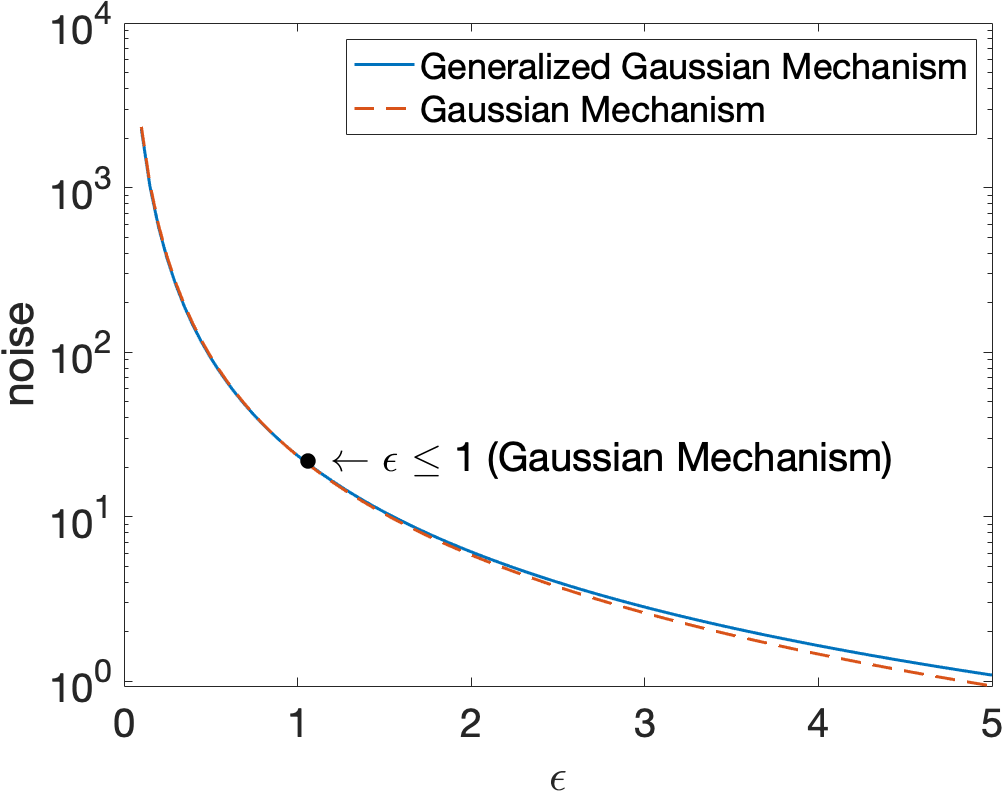 Figure 9
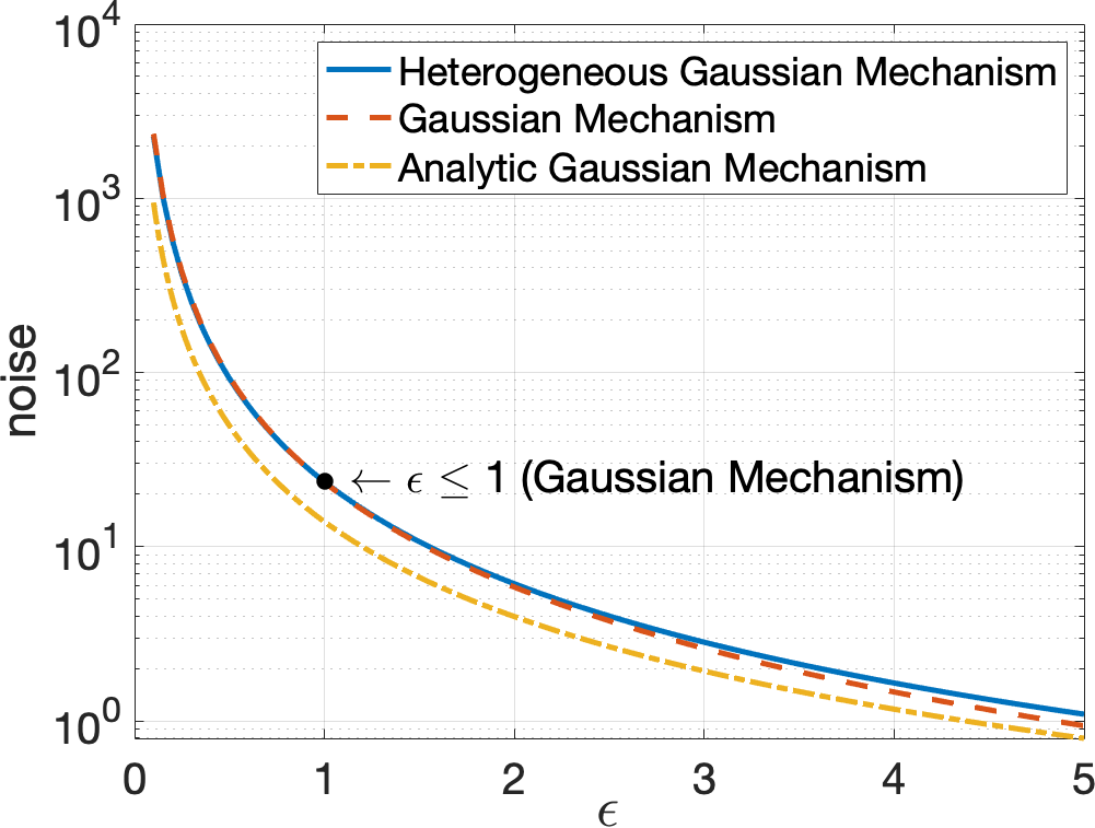 Figure 10
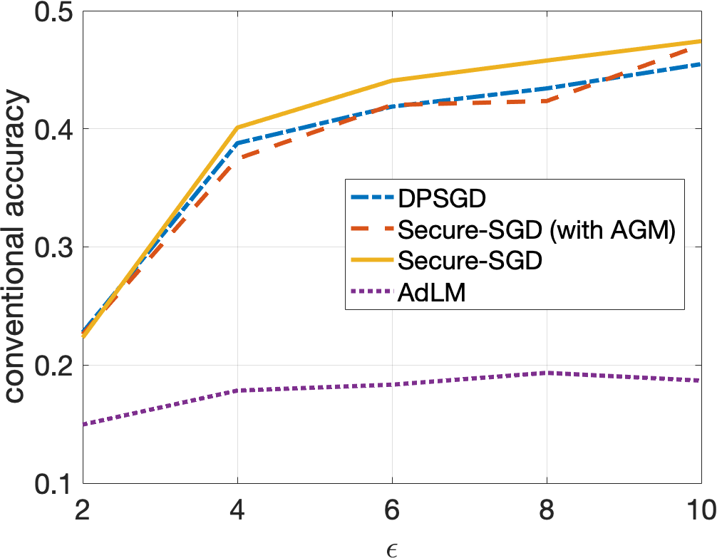 Figure 11
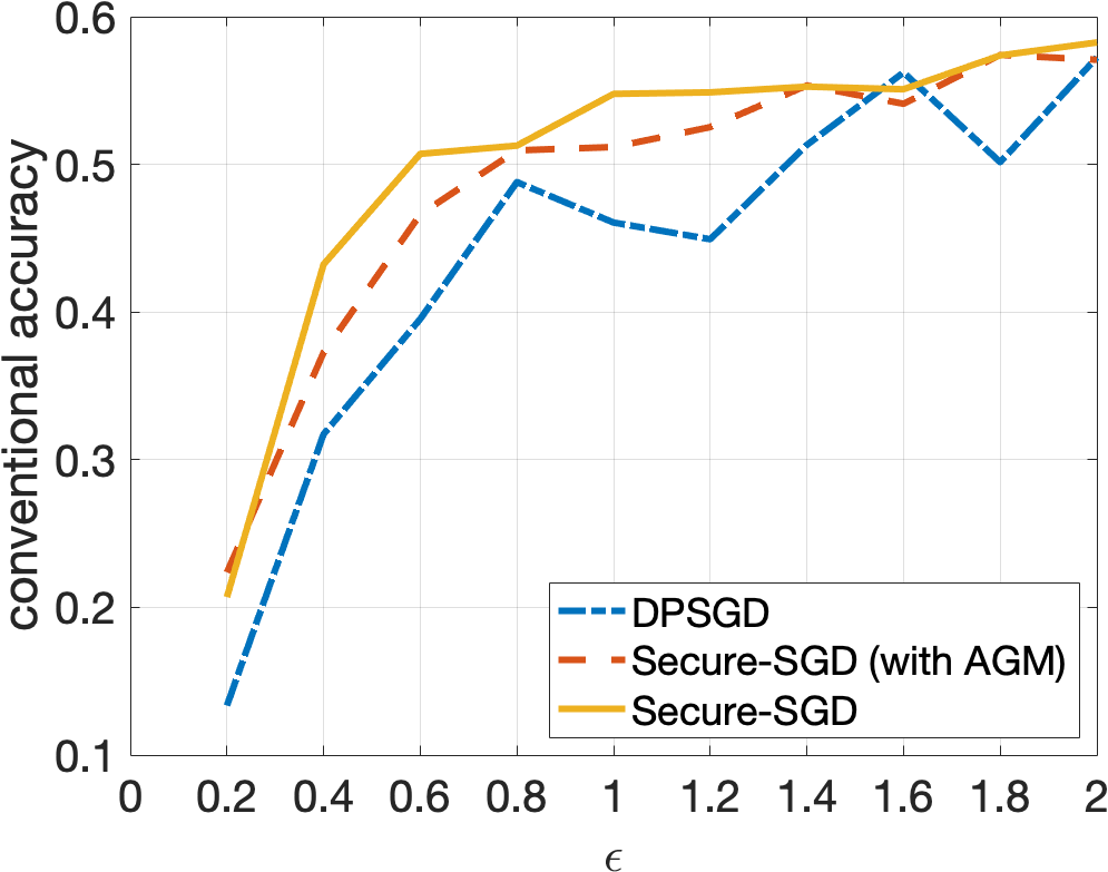 Figure 12
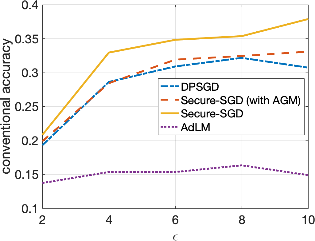 Figure 13
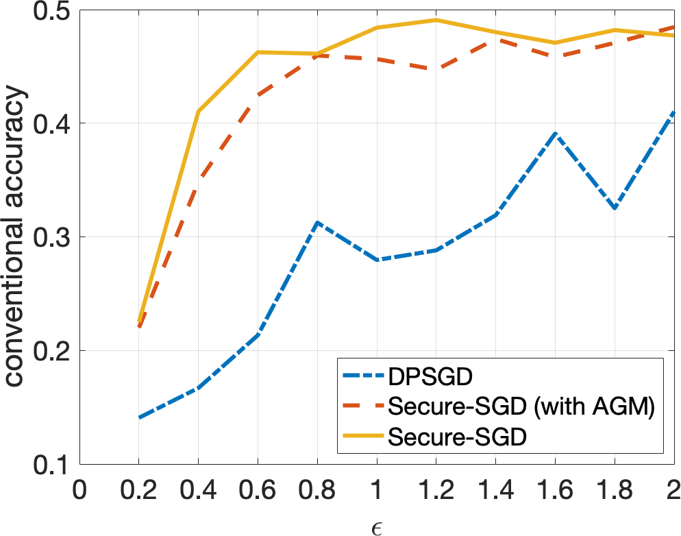 Figure 14
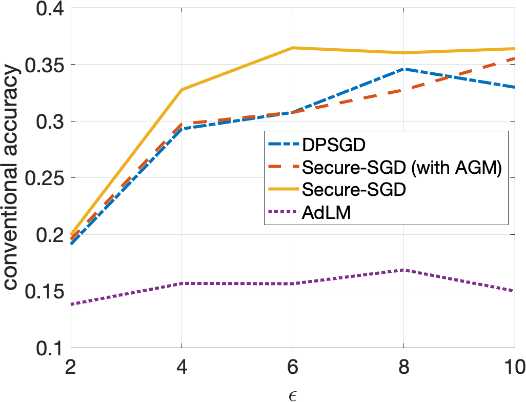 Figure 15
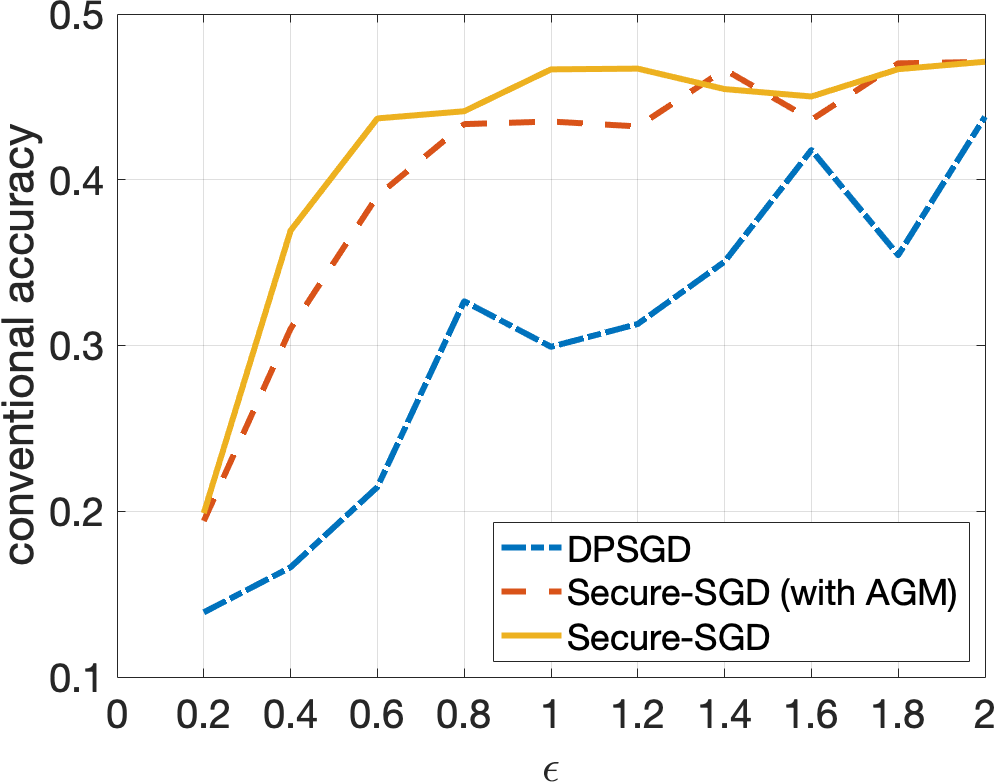 Figure 16
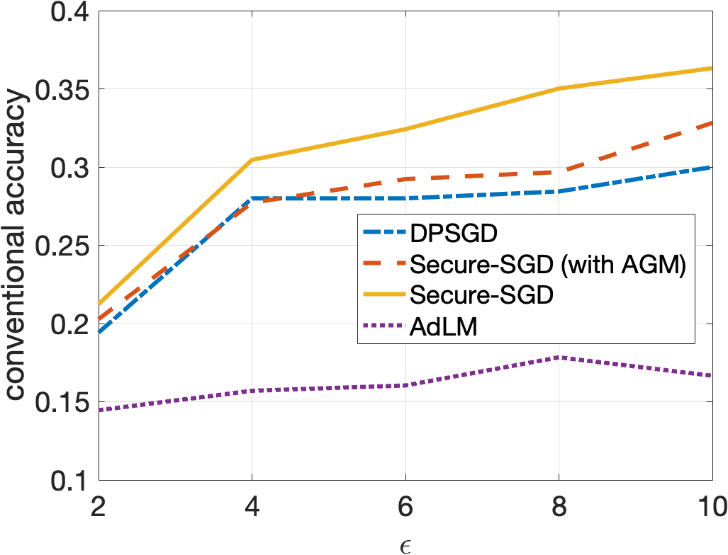 Figure 17
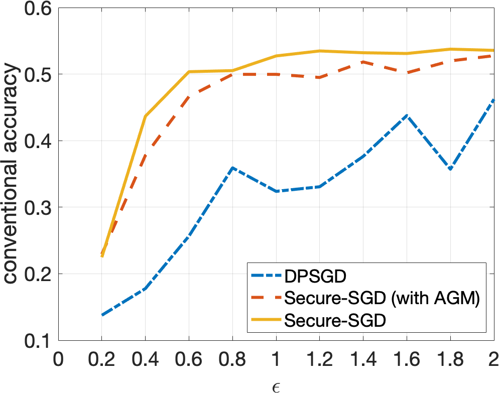 Figure 18
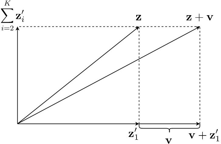 Figure 19
Peer Reviews
No public reviews on file for this paper yet. If you reviewed it on a platform where reviews are public (OpenReview, ICLR, NeurIPS, ICML), you can paste yours below so the community can read it here.
Code & Models
Videos
No videos yet. Explain this paper in a talk, walkthrough, or lecture? Add one.
Heterogeneous Gaussian Mechanism:
Preserving Differential Privacy in Deep Learning with Provable Robustness
NhatHai Phan1111Co-first authors.
Minh Vu5∗
Yang Liu1∗
Ruoming Jin2
Dejing Dou3
Xintao Wu4
My T. Thai5
1New Jersey Institute of Technology, USA; 2Kent State University, USA; 3University of Oregon, USA; 4University of Arkansas, USA; 5University of Florida, USA
{phan,yl558}@njit.edu, {minhvu,mythai}@ufl.edu, [email protected], [email protected], [email protected]
Abstract
In this paper, we propose a novel Heterogeneous Gaussian Mechanism (HGM) to preserve differential privacy in deep neural networks, with provable robustness against adversarial examples. We first relax the constraint of the privacy budget in the traditional Gaussian Mechanism from to , with a new bound of the noise scale to preserve differential privacy. The noise in our mechanism can be arbitrarily redistributed, offering a distinctive ability to address the trade-off between model utility and privacy loss. To derive provable robustness, our HGM is applied to inject Gaussian noise into the first hidden layer. Then, a tighter robustness bound is proposed. Theoretical analysis and thorough evaluations show that our mechanism notably improves the robustness of differentially private deep neural networks, compared with baseline approaches, under a variety of model attacks.
1 Introduction
Recent developments of machine learning (ML) significantly enhance sharing and deploying of ML models in practical applications more than ever before. This presents critical privacy and security issues, when ML models are built on personal data, e.g., clinical records, images, user profiles, etc. In fact, adversaries can conduct: 1) privacy model attacks, in which deployed ML models can be used to reveal sensitive information in the private training data Fredrikson et al. (2015); Wang et al. (2015); Shokri et al. (2017); Papernot et al. (2016); and 2) adversarial example attacks Goodfellow et al. (2014) to cause the models to misclassify. Note that adversarial examples are maliciously perturbed inputs designed to mislead a model at test time Liu et al. (2016); Carlini and Wagner (2017). That poses serious risks to deploy machine learning models in practice. Therefore, it is of paramount significance to simultaneously preserve privacy in the private training data and guarantee the robustness of the model under adversarial examples.
To preserve privacy in the training set, recent efforts have focused on applying Gaussian Mechanism (GM) Dwork and Roth (2014) to preserve differential privacy (DP) in deep learning Abadi et al. (2016); Hamm et al. (2017); Yu et al. (2019); Lee and Kifer (2018). The concept of DP is an elegant formulation of privacy in probabilistic terms, and provides a rigorous protection for an algorithm to avoid leaking personal information contained in its inputs. It is becoming mainstream in many research communities and has been deployed in practice in the private sector and government agencies. DP ensures that the adversary cannot infer any information with high confidence (controlled by a privacy budget and a broken probability ) about any specific tuple from the released results. GM is also applied to derive provable robustness against adversarial examples Lecuyer et al. (2018). However, existing efforts only focus on either preserving DP or deriving provable robustness Kolter and Wong (2017); Raghunathan et al. (2018), but not both DP and robustness!
With the current form of GM Dwork and Roth (2014) applied in existing works Abadi et al. (2016); Hamm et al. (2017); Lecuyer et al. (2018), it is challenging to preserve DP in order to protect the training data, with provable robustness. In GM, random noise scaled to is injected into each of the components of an algorithm output, where the noise scale is a function of , , and the mechanism sensitivity . In fact, there are three major limitations in these works when applying GM: (1) The privacy budget in GM is restricted to , resulting in a limited search space to optimize the model utility and robustness bounds; (2) All the features (components) are treated the same in terms of the amount of noise injected. That may not be optimal in real-world scenarios Bach et al. (2015); Phan et al. (2017); and (3) Existing works have not been designed to defend against adversarial examples, while preserving differential privacy in order to protect the training data. These limitations do narrow the applicability of GM, DP, deep learning, and provable robustness, by affecting the model utility, flexibility, reliability, and resilience to model attacks in practice.
Our Contributions. To address these issues, we first propose a novel Heterogeneous Gaussian Mechanism (HGM), in which (1) the constraint of is extended from to ; (2) a new lower bound of the noise scale will be presented; and more importantly, (3) the magnitude of noise can be heterogeneously injected into each of the features or components. These significant extensions offer a distinctive ability to address the trade-off among model utility, privacy loss, and robustness by redistributing the noise and enlarging the search space for better defensive solutions.
Second, we develop a novel approach, called Secure-SGD, to achieve both DP and robustness in the general scenario, i.e., any value of the privacy budget . In Secure-SGD, our HGM is applied to inject Gaussian noise into the first hidden layer of a deep neural network. This noise is used to derive a tighter and provable robustness bound. Then, DP stochastic gradient descent (DPSGD) algorithm Abadi et al. (2016) is applied to learn differentially private model parameters. The training process of our mechanism preserves DP in deep neural networks to protect the training data with provable robustness. To our knowledge, Secure-SGD is the first approach to learn such a secure model with a high utility. Rigorous experiments conducted on MNIST and CIFAR-10 datasets Lecun et al. (1998); Krizhevsky and Hinton (2009) show that our approach significantly improves the robustness of DP deep neural networks, compared with baseline approaches.
2 Preliminaries and Related Work
In this section, we revisit differential privacy, PixelDP Lecuyer et al. (2018), and introduce our problem definition. Let be a database that contains tuples, each of which contains data and a ground-truth label . Let us consider a classification task with possible categorical outcomes; i.e., the data label given is assigned to only one of the categories. Each can be considered as a one-hot vector of categories . On input and parameters , a model outputs class scores that maps -dimentional inputs to a vector of scores s.t. and . The class with the highest score value is selected as the predicted label for the data tuple, denoted as . We specify a loss function that represents the penalty for mismatching between the predicted values and original values .
Differential Privacy. The definitions of differential privacy and Gaussian Mechanism are as follows:
Definition 1
-Differential Privacy Dwork et al. (2006). A randomized algorithm fulfills -differential privacy, if for any two databases and differing at most one tuple, and for all , we have:
[TABLE]
Smaller and enforce a stronger privacy guarantee.
Here, controls the amount by which the distributions induced by and may differ, and is a broken probability. DP also applies to general metrics , including Hamming metric as in Definition 1 and -norms Chatzikokolakis et al. (2013). Gaussian Mechanism is applied to achieve DP given a random algorithm as follows:
Theorem 1
Gaussian Mechanism Dwork and Roth (2014). Let be an arbitrary -dimensional function, and define its sensitivity to be . The Gaussian Mechanism with parameter adds noise scaled to to each of the components of the output. Given , the Gaussian Mechanism with is -DP.
Adversarial Examples. For some target model and inputs , i.e., is the true label of , one of the adversary’s goals is to find an adversarial example , where is the perturbation introduced by the attacker, such that: (1) and are close, and (2) the model misclassifies , i.e., . In this paper, we consider well-known classes of -norm bounded attacks Goodfellow et al. (2014). Let be the -norm ball of radius . One of the goals in adversarial learning is to minimize the risk over adversarial examples:
[TABLE]
where a specific attack is used to approximate solutions to the inner maximization problem, and the outer minimization problem corresponds to training the model with parameters over these adversarial examples .
We revisit two basic attacks in this paper. The first one is a single-step algorithm, in which only a single gradient computation is required. For instance, Fast Gradient Sign Method (FGSM) algorithm Goodfellow et al. (2014) finds an adversarial example by maximizing the loss function . The second one is an iterative algorithm, in which multiple gradients are computed and updated. For instance, in Kurakin et al. (2016), FGSM is applied multiple times with small steps, each of which has a size of , where is the number of steps.
Provable Robustness and PixelDP. In this paper, we consider the following robustness definition. Given a benign example , we focus on achieving a robustness condition to attacks of -norm, as follows:
[TABLE]
where = , indicating that a small perturbation in the input does not change the predicted label .
To achieve the robustness condition in Eq. 2, Lecuyer et al. (2018) introduce an algorithm, called PixelDP. By considering an input (e.g., images) as databases in DP parlance, and individual features (e.g., pixels) as tuples in DP, PixelDP shows that randomizing the scoring function to enforce DP on a small number of pixels in an image guarantees robustness of predictions against adversarial examples that can change up to that number of pixels. To achieve the goal, noise is injected into either input or some hidden layer of a deep neural network. That results in the following -PixelDP condition, with a budget and a broken brobability of robustness, as follows:
Lemma 1
-PixelDP Lecuyer et al. (2018). Given a randomized scoring function satisfying -PixelDP w.r.t. a -norm metric, we have:
[TABLE]
where is the expected value of .
The network is trained by applying typical optimizers, such as SGD. At the prediction time, a certified robustness check is implemented for each prediction. A generalized robustness condition is proposed as follows:
[TABLE]
where and are the lower bound and upper bound of the expected value , derived from the Monte Carlo estimation with an -confidence, given is the number of invocations of with independent draws in the noise . Passing the check for a given input guarantees that no perturbation exists up to -norm that causes the model to change its prediction result. In other words, the classification model, based on , i.e., , is consistent to attacks of -norm on with probability . Group privacy Dwork et al. (2006) can be applied to achieve the same robustness condition, given a particular size of perturbation . For a given , , and sensitivity used at prediction time, PixelDP solves for the maximum for which the robustness condition in Eq. 4 checks out:
[TABLE]
3 Heterogeneous Gaussian Mechanism
We now formally present our Heterogeneous Gaussian Mechanism (HGM) and the Secure-SGD algorithm. In Eq. 5, it is clear that is restricted to be , following the Gaussian Mechanism (Theorem 1). That affects the robustness bound in terms of flexibility, reliability, and utility. In fact, adversaries only need to guarantee that is larger than at most , i.e., , in order to assault the robustness condition: thus, softening the robustness bound. In addition, the search space for the robustness bound is limited, given . These issues increase the number of robustness violations, potentially degrading the utility and reliability of the robustness bound. In real-world applications, such as healthcare, autonomous driving, object recognition, etc., a flexible value of is needed to implement stronger and more practical robustness bounds. This is also true for many other algorithms applying Gaussian Mechanism Dwork and Roth (2014).
To relax this constraint, we introduce an Extended Gaussian Mechanism as follows:
Theorem 2
Extended Gaussian Mechanism. Let be an arbitrary -dimensional function, and define its sensitivity to be . An Extended Gaussian Mechanism with parameter adds noise scaled to to each of the components of the output. The mechanism is -DP, with
[TABLE]
Detailed proof of Theorem 2 is in Appendix A222https://www.dropbox.com/s/mjkq4zqqh6ifqir/HGM_Appendix.pdf?dl=0. The Extended Gaussian Mechanism enables us to relax the constraint of . However, the noise scale is used to inject Gaussian noise into each component. This may not be optimal, since different components usually have different impacts to the model outcomes Bach et al. (2015). To address this, we further propose a Heterogeneous Gaussian Mechanism (HGM), in which the noise scale in Theorem 2 can be arbitrarily redistributed. Different strategies can be applied to improve the model utility and to enrich the search space for better robustness bounds. For instance, more noise will be injected into less important components, or vice-versa, or even randomly redistributed. In order to achieve our goal, we introduce a noise redistribution vector , where that satisfies and . We show that by injecting Gaussian noise \mathcal{N}\big{(}0,\sigma^{2}K\mathbf{r}\big{)}, where \Delta_{A}=\max_{D,D^{\prime}}\sqrt{\sum_{k=1}^{K}\frac{1}{Kr_{k}}\big{(}A(D)_{k}-A(D^{\prime})_{k}\big{)}^{2}} and , we achieve -DP.
Theorem 3
Heterogeneous Gaussian Mechanism. Let be an arbitrary -dimensional function, and define its sensitivity to be \Delta_{A}=\max_{D,D^{\prime}}\lVert\frac{A(D)-A(D^{\prime})}{\sqrt{K\mathbf{r}}}\rVert_{2}=\max_{D,D^{\prime}}\sqrt{\sum_{k=1}^{K}\frac{1}{Kr_{k}}\big{(}A(D)_{k}-A(D^{\prime})_{k}\big{)}^{2}}. A Heterogeneous Gaussian Mechanism with parameter adds noise scaled to to each of the components of the output. The mechanism is -DP, with
[TABLE]
where s.t. and .
Detailed proof of Theorem 3 is in Appendix B1. It is clear that the Extended Gaussian Mechanism is a special case of the HGM, when . Figure 1 illustrates the magnitude of noise injected by the traditional Gaussian Mechanism, the state-of-the-art Analytic Gaussian Mechanism Balle and Wang (2018), and our Heterogeneous Gaussian Mechanism as a function of , given the global sensitivity , and (a very tight broken probability), and . The lower bound of the noise scale in our HGM is just a little bit better than the traditional Gaussian Mechanism when . However, our mechanism does not have the constraint on the privacy budget . The Analytic Gaussian Mechanism Balle and Wang (2018), which provides the state-of-the-art noise bound, has a better noise scale than our mechanism. However, our noise scale bound provides a distinctive ability to redistribute the noise via the vector , compared with the Analytic Gaussian Mechanism. There could be numerous strategies to identify vector . This is significant when addressing the trade-off between model utility and privacy loss or robustness in real-world applications. In our mechanism, “more noise” is injected into “more vulnerable” components to improve the robustness. We will show how to compute vector and identify vulnerable components in our Secure-SGD algorithm. Experimental results illustrate that, by redistributing the noise, our HGM yields better robustness, compared with existing mechanisms.
4 Secure-SGD
In this section, we focus on applying our HGM in a crucial and emergent application, which is enhancing the robustness of differentially private deep neural networks. Given a deep neural network , DPSGD algorithm Abadi et al. (2016) is applied to learn -DP parameters . Then, by injecting Gaussian noise into the first hidden layer, we can leverage the robustness concept of PixelDP Lecuyer et al. (2018) (Eq. 5) to derive a better robustness bound based on our HGM.
Algorithm 1 outlines the key steps in our Secure-SGD algorithm. We first initiate the parameters and construct a deep neural network (Lines 1-2). Then, a robustness noise is drawn by applying our HGM (Line 3), where is computed following Theorem 3, is the number of hidden neurons in , denoted as , and is the sensitivity of the algorithm, defined as the maximum change in the output (i.e., which is ) that can be generated by the perturbation in the input under the noise redistribution vector .
[TABLE]
For -norm attacks, we use the following bound , where is the maximum 1-norm of ’s rows over the vector . The vector can be computed as the forward derivative of as follows:
[TABLE]
where is a user-predefined inflation rate. It is clear that features, which have higher forward derivative values, will be more vulnerable to attacks by maximizing the loss function . These features are assigned larger values in vector , resulting in more noise injected, and vice-versa. The computation of can be considered as a prepossessing step using a pre-trained model. It is important to note that the utilizing of does not risk any privacy leakage, since is only applied to derive provable robustness. It does not have any effect on the DP-preserving procedure in our algorithm, as follows. First, at each training step , our mechanism takes a random sample from the data , with sampling probability , where is a batch size (Line 5). For each tuple , the first hidden layer is perturbed by adding Gaussian noise derived from our HGM (Line 6, Alg. 1):
[TABLE]
This ensures that the scoring function satisfies -PixelDP (Lemma 3). Then, the gradient is computed (Lines 7-9). The gradients will be bounded by clipping each gradient in norm; i.e., the gradient vector is replaced by for a predefined threshold (Lines 10-12). Uniformed normal distribution noise is added into gradients of parameters (Line 14), as:
[TABLE]
The descent of the parameters explicitly is as: , where is a learning rate at the step (Line 16). The training process of our mechanism achieves both -DP to protect the training data and provable robustness with the budgets . In the verified testing phase (Lines 17-22), by applying HGM and PixelDP, we derive a novel robustness bound for a specific input as follows:
[TABLE]
where and are the lower and upper bounds of the expected value , derived from the Monte Carlo estimation with an -confidence, given is the number of invocations of with independent draws in the noise . Similar to Lecuyer et al. (2018), we use Hoeffding’s inequality Hoeffding (1963) to bound the error in . If the robustness size is larger than a given adversarial perturbation size , the model prediction is considered consistent to that attack size. Given the relaxed budget and the noise redistribution , the search space for the robustness size is significantly enriched, e.g., , strengthening the robustness bound. Note that vector can also be randomly drawn in the estimation of the expected value . Both fully-connected and convolution layers can be applied. Given a convolution layer, we need to ensure that the computation of each feature map is -PixelDP, since each of them is independently computed by reading a local region of input neurons. Therefore, the sensitivity can be considered the upper-bound sensitivity given any single feature map. Our algorithm is the first effort to connect DP preservation in order to protect the original training data and provable robustness in deep learning.
5 Experimental Results
We have carried out extensive experiments on two benchmark datasets, MNIST and CIFAR-10. Our goal is to evaluate whether our HGM significantly improves the robustness of both differentially private and non-private models under strong adversarial attacks, and whether our Secure-SGD approach retains better model utility compared with baseline mechanisms, under the same DP guarantees and protections.
Baseline Approaches. Our HGM and two approaches, including HGM_PixelDP and Secure-SGD, are evaluated in comparison with state-of-the-art mechanisms in: (1) DP-preserving algorithms in deep learning, i.e., DPSGD Abadi et al. (2016), AdLM Phan et al. (2017); in (2) Provable robustness, i.e., PixelDP Lecuyer et al. (2018); and (3) The Analytic Gaussian Mechanism (AGM) Balle and Wang (2018). To preserve DP, DPSGD injects random noise into gradients of parameters, while AdLM is a Functional Mechanism-based approach. PixelDP is one of the state-of-the-art mechanisms providing provable robustness using DP bounds. Our HGM_PixelDP model simply is PixelDP with the noise bound derived from our HGM. The baseline models share the same design in our experiment. We consider the class of -bounded adversaries. Four white-box attack algorithms were used, including FGSM, I-FGSM, Momentum Iterative Method (MIM) Dong et al. (2017), and MadryEtAl Madry et al. (2018), to draft adversarial examples .
MNIST: We used two convolution layers (32 and 64 features). Each hidden neuron connects with a 5x5 unit patch. A fully-connected layer has 256 units. The batch size was set to 128, , , , and . CIFAR-10: We used three convolution layers (128, 128, and 256 features). Each hidden neuron connects with a 3x3 unit patch in the first layer, and a 5x5 unit patch in other layers. One fully-connected layer has 256 neurons. The batch size was set to 128, , , , and . Note that is used to indicate the DP budget used to protect the training data; meanwhile, is the budget for robustness. The implementation of our mechanism is available in TensorFlow333https://github.com/haiphanNJIT/SecureSGD. We apply two accuracy metrics as follows:
[TABLE]
where is the number of test cases, returns if the model makes a correct prediction (otherwise, returns 0), and returns if the robustness size is larger than a given attack bound (otherwise, returns 0).
HGM_PixelDP. Figures 2 and 3 illustrate the certified accuracy under attacks of each model as a function of the adversarial perturbation . Our HGM_PixelDP notably outperforms the PixelDP model in most of the cases given the CIFAR-10 dataset. We register an improvement of 8.63% on average when compared with the PixelDP, i.e., (2 tail t-test). This clearly shows the effectiveness of our HGM in enhancing the robustness against adversarial examples. Regarding the MNIST data, our HGM_PixelDP model achieves better certified accuracies when compared with the PixelDP model. On average, our HGM_PixelDP () improves 4.17% in terms of certified accuracy given , compared with the PixelDP, (2 tail t-test). Given very strong adversarial perturbation , smaller usually yields better results, offering the flexibility in choosing appropriate DP budget for robustness given different attack magnitudes. These experimental results clearly show crucial benefits of relaxing the constraints of the privacy budget and of the heterogeneous noise distribution in our HGM.
Secure-SGD. The application of our HGM in DP-preserving deep neural networks, i.e., Secure-SGD, further strengthens our observations. Figures 4 and 5 illustrate the certified accuracy under attacks of each model as a function of the privacy budget used to protect the training data. By incorporating HGM into DPSGD, our Secure-SGD remarkably increases the robustness of differentially private deep neural networks. In fact, our Secure-SGD with HGM outmatches DGSGP, AdLM, and the application of AGM in our Secure-SGD algorithm in most of the cases. Note that the application of AGM in our Secure-SGD does not redistribute the noise in deriving the provable robustness. In CIFAR-10 dataset, our Secure-SGD () correspondingly acquires a 2.7% gain (, 2 tail t-test), a 3.8% gain (, 2 tail t-test), and a 17.75% gain (, 2 tail t-test) in terms of conventional accuracy, compared with AGM in Secure-SGD, DPSGD, and AdLM algorithms. We register the same phenomenon in the MNIST dataset. On average, our Secure-GSD () correspondingly outperforms the AGM in Secure-SGD and DPSGD with an improvement of 2.9% (, 2 tail t-test) and an improvement of 10.74% (, 2 tail t-test).
Privacy Preserving and Provable Robustness. We also discover an original, interesting, and crucial trade-off between DP preserving to protect the training data and the provable robustness (Figures 4 and 5). Given our Secure-SGD model, there is a huge improvement in terms of conventional accuracy when the privacy budget increases from 0.2 to 2 in MNIST dataset (i.e., 29.67% on average), and from 2 to 10 in CIFAR-10 dataset (i.e., 18.17% on average). This opens a long-term research avenue to achieve better provable robustness under strong privacy guarantees, since with strong privacy guarantees (i.e., small values of ), the conventional accuracies of all models are still modest.
6 Conclusion
In this paper, we presented a Heterogeneous Gaussian Mechanism (HGM) to relax the privacy budget constraint, i.e., from to , and its heterogeneous noise bound. An original application of our HGM in DP-preserving mechanism with provable robustness was designed to enhance the robustness of DP deep neural networks, by introducing a novel Secure-SGD algorithm with a better robustness bound. Our model shows promising results and opens a long-term avenue to address the trade-off between DP preservation and provable robustness. In future work, we will learn how to identify and incorporate more practical Gaussian noise distributions to further improve the model accuracies under model attacks.
Acknowledgement
This work is partially supported by grants DTRA HDTRA1-14-1-0055, NSF CNS-1850094, NSF CNS-1747798, NSF IIS-1502273, and NJIT Seed Grant.
Appendix A Proof of Theorem 2
Proof 1
The privacy loss of the Extended Gaussian Mechanism incurred by observing an output is defined as:
[TABLE]
Given , we have that
[TABLE]
where .
Since \mathbf{o}-A(D)\sim\mathcal{N}\big{(}0,\sigma^{2}{\Delta}^{2}_{A}\big{)}, then \mathbf{z}\sim\mathcal{N}\big{(}0,\sigma^{2}{\Delta}^{2}_{A})\big{)}. Now we will use the fact that the distribution of a spherically symmetric normal is independent of the orthogonal basis, from which its constituent normals are drawn. Then, we work in a basis that is aligned with .
Let be a basis that satisfies and . Fix such a basis , we draw by first drawing signed lengths \lambda_{i}\sim\mathcal{N}\big{(}0,\sigma^{2}{\Delta}^{2}_{A}\big{)}~{}(i\in[1,K]). Then, let and . Without loss of generality, let us assume that is parallel to . Consider that the triangle with base and the edge is orthogonal to . The hypotenuse of this triangle is (Figure 6). Then we have
[TABLE]
Since is parallel to , we have . Then we have
[TABLE]
By bounding the privacy loss by , we have
[TABLE]
Let . To ensure the privacy loss is bounded by with probability at least , we require
[TABLE]
Recall that , we have that
[TABLE]
Then, we have
[TABLE]
Next we will use the tail bound: . We require:
[TABLE]
Taking , we have that
[TABLE]
We will ensure the above inequality by requiring: (1) , and (2) \frac{1}{2}\big{(}\frac{2\sigma^{2}\epsilon-1}{2\sigma}\big{)}^{2}\geq\ln(\sqrt{\frac{2}{\pi}}\frac{1}{\delta}).
[TABLE]
We can ensure this inequality (Eq. 15) by setting:
[TABLE]
Let . If , the second requirement will always be satisfied, and we only need to choose satisfying the Condition 1. When , since we already ensure , we have that
[TABLE]
We can ensure the above inequality by choosing:
[TABLE]
Based on the proof above, now we know that to ensure the privacy loss bounded by with probability at least , we require:
[TABLE]
To compare Condition 2 and Condition 1, we have that
[TABLE]
Since usually is a very small number, i.e., -, without loss of generality, we can assume that Condition 2 always implies Condition 1 in practice. To ensure the privacy loss bounded by with probability at least , only Condition 2 needs to be satisfied:
[TABLE]
In this proof, the noise is injected into the model. If we set , then the noise becomes . Consequently, Theorem 2 does hold.
Appendix B Proof of Theorem 3
Proof 2
The privacy loss of the Heterogeneous Gaussian Mechanism incurred by observing an output is defined as:
[TABLE]
Given , we have that
[TABLE]
Let be a -dimensional vector that satisfies Let be a -dimensional vector that satisfies . Then we have that
[TABLE]
Since \mathbf{o}-A(D)\sim\mathcal{N}\big{(}0,\sigma^{2}{\Delta}^{2}_{A}K\mathbf{r}\big{)}, then \mathbf{z}\sim\mathcal{N}\big{(}0,\sigma^{2}\Delta^{2}_{A}\big{)}. Now we will use the fact that the distribution of a spherically symmetric normal is independent of the orthogonal basis from which its constituent normals are drawn. Then, we work in a basis that is aligned with .
Let be a basis that satisfies and . Fix such a basis , we draw by first drawing signed lengths \lambda_{k}\sim\mathcal{N}\big{(}0,\sigma^{2}{\Delta}^{2}_{A}\big{)}~{}(k\in[K]). Then, let , and finally let . Assume without loss of generality that is parallel to . Consider that the right triangle with base and edge orthogonal to . The hypotenuse of this triangle is (Figure 6). Then we have
[TABLE]
Since is parallel to , we have . Then we have
[TABLE]
By bounding the privacy loss by , we have
[TABLE]
Let . To ensure the privacy loss is bounded by with probability at least , we require
[TABLE]
Recall that , we have that
[TABLE]
Then, we have
[TABLE]
Next we will use the tail bound: . We require:
[TABLE]
Taking , we have that
[TABLE]
We will ensure the above inequality by requiring: (1) , and (2) \frac{1}{2}\big{(}\frac{2\sigma^{2}\epsilon-1}{2\sigma}\big{)}^{2}\geq\ln(\sqrt{\frac{2}{\pi}}\frac{1}{\delta}).
[TABLE]
We can ensure this inequality (Eq. 26) by setting:
[TABLE]
Let . If , the second requirement will always be satisfied, and we only need to choose satisfying the Condition 1. When , since we already ensure , we have that
[TABLE]
We can ensure the above inequality by choosing:
[TABLE]
Based on the proof above, now we know that to ensure the privacy loss bounded by with probability at least , we require:
[TABLE]
To compare Condition 2 and Condition 1, we have that
[TABLE]
Since usually is a very small number, i.e., -, without loss of generality, we can assume that Condition 2 always implies Condition 1 in practice. To ensure the privacy loss bounded by with probability at least , only Condition 2 needs to be satisfied:
[TABLE]
In this proof, the noise is injected into the model. If we set , then the noise becomes . Consequently, Theorem 3 does hold.
The reference list from the paper itself. Each links out to its DOI / PubMed record.
- 1Abadi et al. [2016] Martin Abadi, Andy Chu, Ian Goodfellow, H. Brendan Mc Mahan, Ilya Mironov, Kunal Talwar, and Li Zhang. Deep learning with differential privacy. ar Xiv:1607.00133 , 2016.
- 2Bach et al. [2015] Sebastian Bach, Alexander Binder, Grégoire Montavon, Frederick Klauschen, Klaus-Robert Müller, and Wojciech Samek. On pixel-wise explanations for non-linear classifier decisions by layer-wise relevance propagation. P Lo S ONE , 10(7):e 0130140, 07 2015.
- 3Balle and Wang [2018] Borja Balle and Yu-Xiang Wang. Improving the Gaussian mechanism for differential privacy: Analytical calibration and optimal denoising. In Jennifer Dy and Andreas Krause, editors, Proceedings of the 35th International Conference on Machine Learning , volume 80 of Proceedings of Machine Learning Research , pages 394–403, Stockholmsmässan, Stockholm Sweden, 10–15 Jul 2018. PMLR.
- 4Carlini and Wagner [2017] N. Carlini and D. Wagner. Towards evaluating the robustness of neural networks. In 2017 IEEE Symposium on Security and Privacy (SP) , pages 39–57, May 2017.
- 5Chatzikokolakis et al. [2013] Konstantinos Chatzikokolakis, Miguel E. Andrés, Nicolás Emilio Bordenabe, and Catuscia Palamidessi. Broadening the scope of differential privacy using metrics. In Emiliano De Cristofaro and Matthew Wright, editors, Privacy Enhancing Technologies , pages 82–102, 2013.
- 6Dong et al. [2017] Yinpeng Dong, Fangzhou Liao, Tianyu Pang, Xiaolin Hu, and Jun Zhu. Discovering adversarial examples with momentum. Co RR , abs/1710.06081, 2017.
- 7Dwork and Roth [2014] Cynthia Dwork and Aaron Roth. The algorithmic foundations of differential privacy. Foundations and Trends® in Theoretical Computer Science , 9(3–4):211–407, 2014.
- 8Dwork et al. [2006] C. Dwork, F. Mc Sherry, K. Nissim, and A. Smith. Calibrating noise to sensitivity in private data analysis. Theory of Cryptography , pages 265–284, 2006.
