Semi- and Weakly-supervised Human Pose Estimation
Norimichi Ukita, Yusuke Uematsu
TL;DR
This paper introduces semi- and weakly-supervised learning methods for human pose estimation that reduce the need for extensive annotated data by leveraging action labels and pose clustering techniques.
Contribution
It proposes three novel learning schemes that improve pose estimation accuracy using limited annotations and action labels, including outlier detection and pose clustering.
Findings
Effective pose estimation with limited labeled data
Improved true-positive pose selection accuracy
Ability to detect diverse poses beyond supervised examples
Abstract
For human pose estimation in still images, this paper proposes three semi- and weakly-supervised learning schemes. While recent advances of convolutional neural networks improve human pose estimation using supervised training data, our focus is to explore the semi- and weakly-supervised schemes. Our proposed schemes initially learn conventional model(s) for pose estimation from a small amount of standard training images with human pose annotations. For the first semi-supervised learning scheme, this conventional pose model detects candidate poses in training images with no human annotation. From these candidate poses, only true-positives are selected by a classifier using a pose feature representing the configuration of all body parts. The accuracies of these candidate pose estimation and true-positive pose selection are improved by action labels provided to these images in our second…
Click any figure to enlarge with its caption.
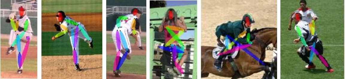 Figure 1
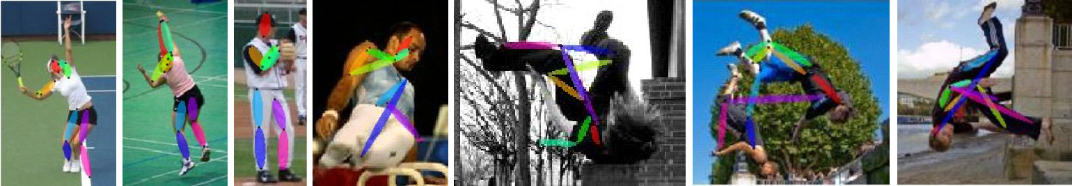 Figure 2
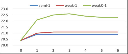 Figure 3
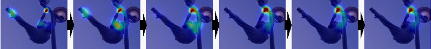 Figure 4
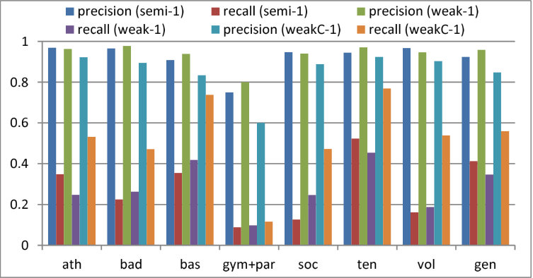 Figure 5
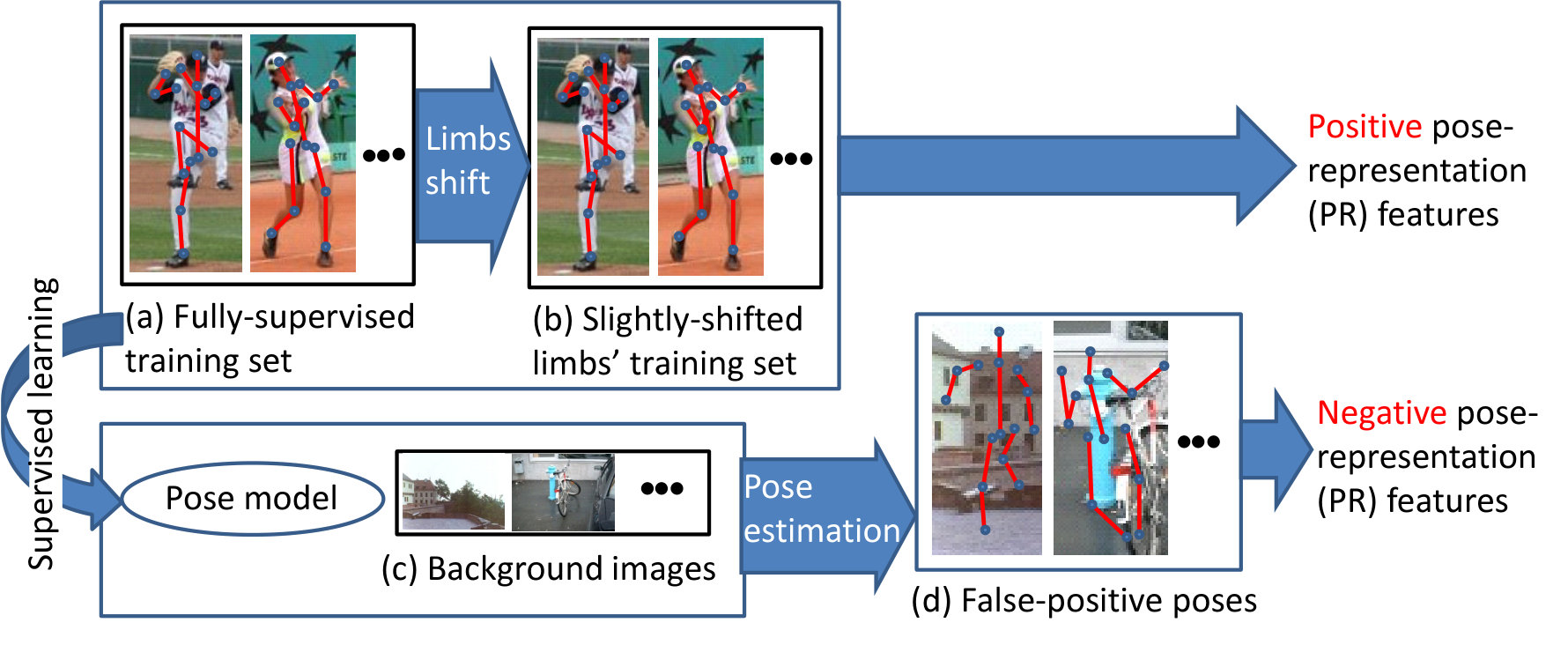 Figure 6
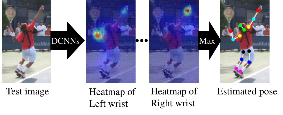 Figure 7
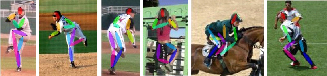 Figure 8
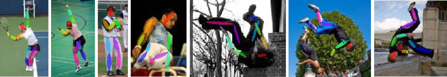 Figure 9
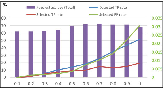 Figure 10
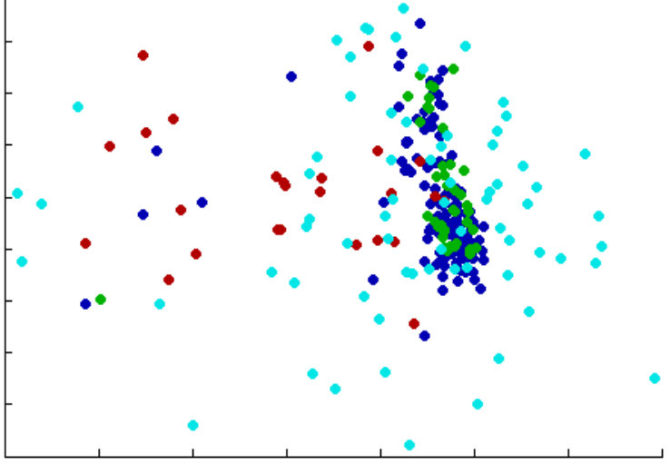 Figure 11
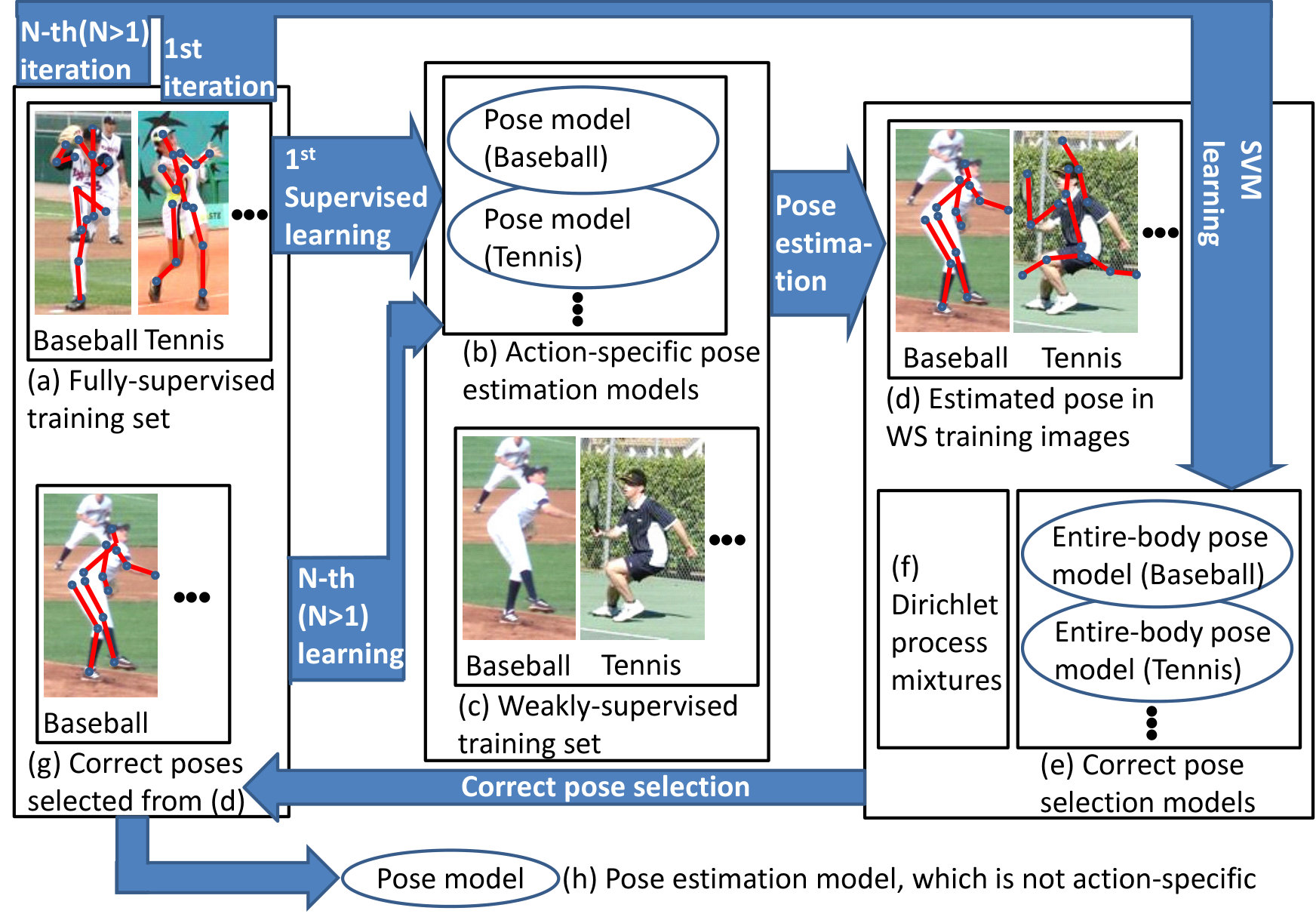 Figure 12
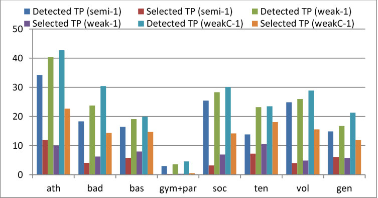 Figure 13
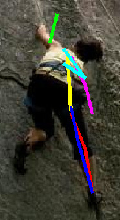 Figure 14
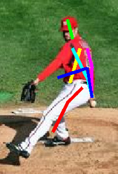 Figure 15
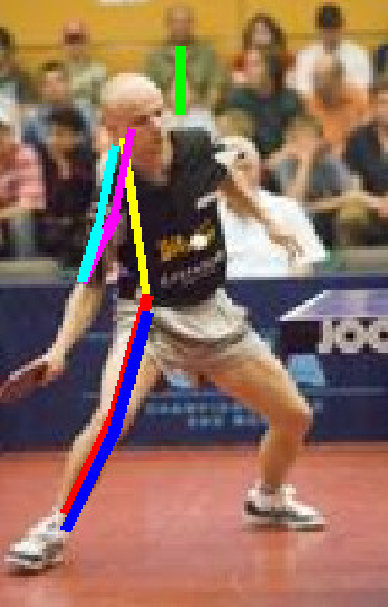 Figure 16
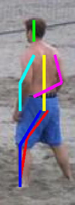 Figure 17
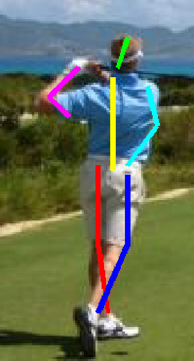 Figure 18
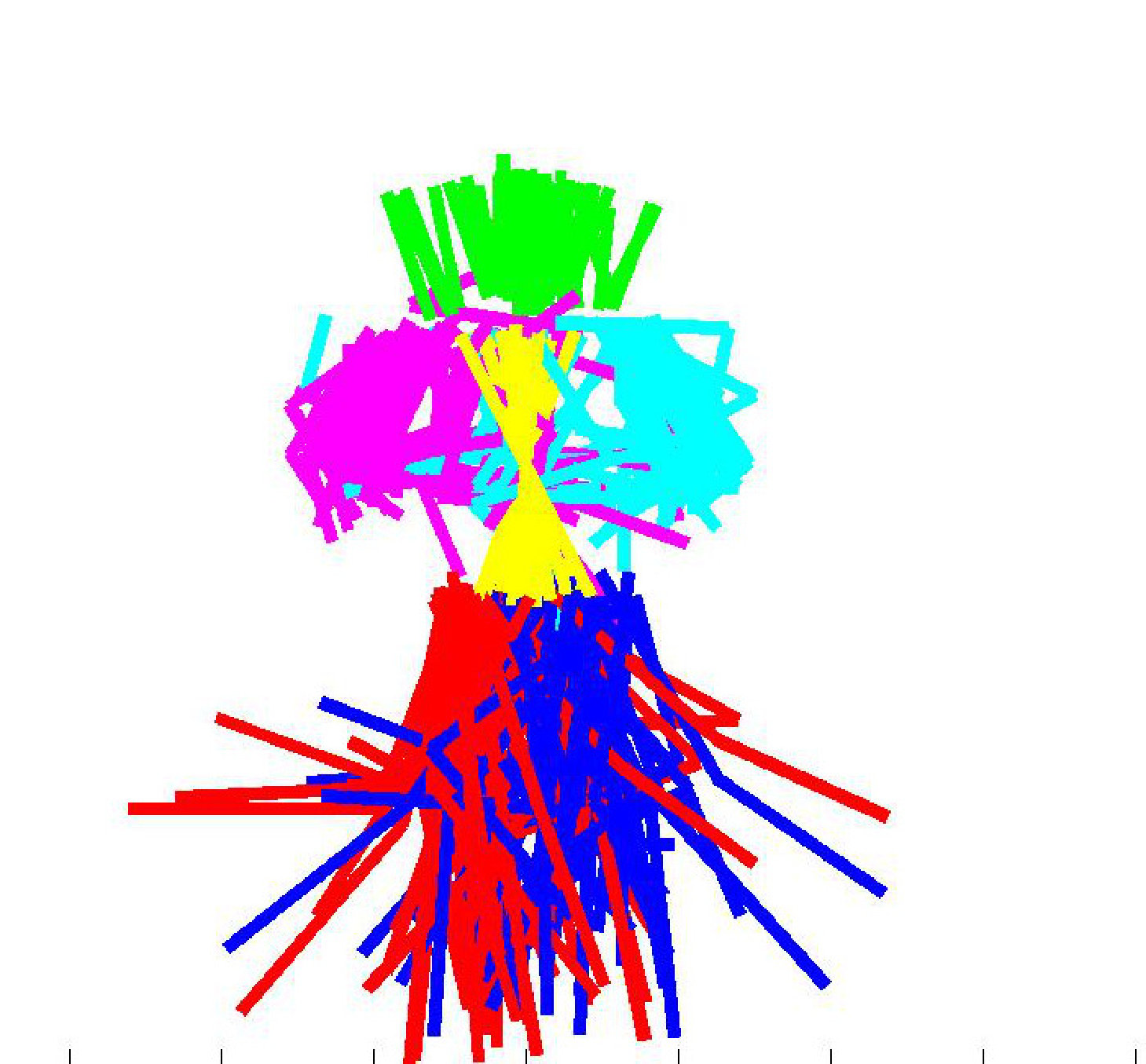 Figure 19
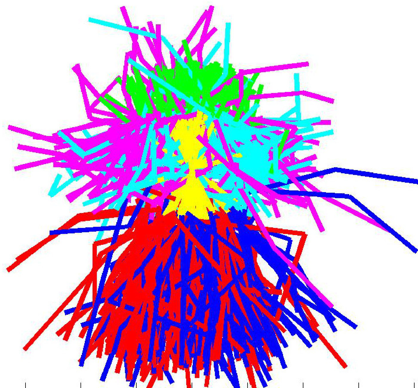 Figure 20
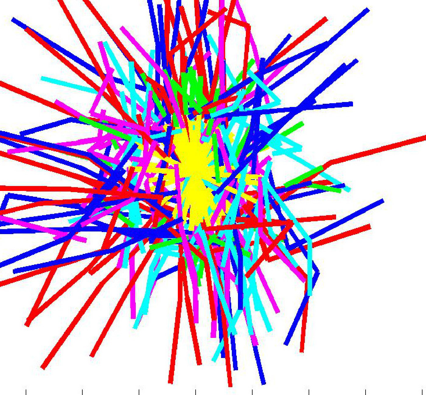 Figure 21
| Athletics | Badminton | Baseball | Gym+Parkour | ||
|---|---|---|---|---|---|
| LSP | Train (FS) | 20 | 62 | 74 | 46 |
| Train (WS) | 13 | 68 | 85 | 57 | |
| Test | 46 | 127 | 137 | 128 | |
| LSP ext | Train | 543 | 1 | 101 | 8547 |
| MPII | Train | 284 | 83 | 208 | 205 |
| Soccer | Tennis | Volleyball | General | ||
| LSP | Train (FS) | 71 | 51 | 40 | 136 |
| Train (WS) | 56 | 47 | 36 | 138 | |
| Test | 125 | 93 | 87 | 257 | |
| LSP ext | Train | 15 | 1 | 4 | 788 |
| MPII | Train | 149 | 176 | 105 | 26735 |
| Method | Head | Shoulder | Elbow | Wrist | Hip | Knee | Ankle | Mean |
|---|---|---|---|---|---|---|---|---|
| LSP | ||||||||
| (a) Tompson et al. [13] | 90.6 | 79.2 | 67.9 | 63.4 | 69.5 | 71.0 | 64.2 | 72.3 |
| (b) Fan et al. [59] | 92.4 | 75.2 | 65.3 | 64.0 | 75.7 | 68.3 | 70.4 | 73.0 |
| (c) Carreira et al. [17] | 90.5 | 81.8 | 65.8 | 59.8 | 81.6 | 70.6 | 62.0 | 73.1 |
| (d) Yang et al. [47] | 90.6 | 78.1 | 73.8 | 68.8 | 74.8 | 69.9 | 58.9 | 73.6 |
| (e) Baseline–1 [11] (HALF) | 88.8 | 75.7 | 69.3 | 61.9 | 71.2 | 67.0 | 58.8 | 70.4 |
| (f) Baseline–1 [11] | 91.8 | 78.2 | 71.8 | 65.5 | 73.3 | 70.2 | 63.4 | 73.4 |
| (g) Ours-semi–1 | 89.0 | 77.8 | 69.7 | 61.9 | 71.8 | 67.4 | 58.9 | 70.9 |
| (h) Ours-weak–1 | 89.0 | 78.0 | 70.0 | 61.7 | 72.1 | 67.8 | 58.9 | 71.1 |
| (i) Ours-weakC–1 | 91.5 | 78.0 | 71.1 | 62.6 | 73.1 | 68.7 | 62.3 | 72.5 |
| (j) Baseline–2 [18] (HALF) | 89.1 | 75.8 | 61.9 | 58.6 | 71.7 | 64.8 | 58.9 | 68.7 |
| (k) Baseline–2 [18] | 93.5 | 83.1 | 69.7 | 68.9 | 81.4 | 73.7 | 65.0 | 76.5 |
| (l) Ours-semi–2 | 90.2 | 77.4 | 62.5 | 58.6 | 73.0 | 64.5 | 58.4 | 69.2 |
| (m) Ours-weak–2 | 90.7 | 78.0 | 63.2 | 59.2 | 74.1 | 66.3 | 58.4 | 70.0 |
| (n) Ours-weakC–2 | 92.1 | 82.0 | 67.6 | 63.3 | 78.8 | 70.6 | 60.5 | 73.6 |
| LSP+LSPext | ||||||||
| (o) Yu et al. [72] | 87.2 | 88.2 | 82.4 | 76.3 | 91.4 | 85.8 | 78.7 | 84.3 |
| (p) Baseline–2 [18] | 96.9 | 87.1 | 80.4 | 75.1 | 86.5 | 83.2 | 81.0 | 84.3 |
| (q) Ours-semi–2 | 91.9 | 79.2 | 67.8 | 60.5 | 79.9 | 70.4 | 63.5 | 73.3 |
| (r) Ours-weak–2 | 93.2 | 81.8 | 69.0 | 61.5 | 83.7 | 71.7 | 64.7 | 75.1 |
| (s) Ours-weakC–2 | 94.0 | 84.4 | 74.7 | 68.7 | 83.0 | 79.8 | 72.1 | 79.5 |
| LSP+LSPext+MPII | ||||||||
| (t) Pishchulin et al. [73] | 97.0 | 91.0 | 83.8 | 78.1 | 91.0 | 86.7 | 82.0 | 87.1 |
| (u) Insafutdinov et al. [74] | 97.4 | 92.7 | 87.5 | 84.4 | 91.5 | 89.9 | 87.2 | 90.1 |
| (v) Baseline–2 [18] | 97.8 | 92.5 | 87.0 | 83.9 | 91.5 | 90.8 | 89.9 | 90.5 |
| (w) Ours-semi–2 | 92.4 | 80.8 | 70.3 | 65.7 | 82.5 | 73.3 | 68.8 | 76.3 |
| (x) Ours-weak–2 | 93.0 | 82.2 | 73.2 | 69.5 | 83.9 | 77.5 | 72.1 | 77.5 |
| (y) Ours-weakC–2 | 93.6 | 85.1 | 76.3 | 71.0 | 85.2 | 80.6 | 77.8 | 81.4 |
| Athletics | Badminton | Baseball | Gym+Parkour | |
| (j) Baseline–2 [18] (HALF) | 68.6 | 66.7 | 67.5 | 69.5 |
| (v) Baseline–2 [18] (LSP+LSPext+MPII) | 91.6 | 90.7 | 90.8 | 91.0 |
| (y) Ours-weakC–2 (LSP+LSPext+MPII) | 84.8 | 75.4 | 80.2 | 80.5 |
| Baseline–2 Gain [(j) (v)] % | 23.0 | 24.0 | 23.3 | 21.5 |
| Ours-weakC–2 Gain [(j) (y)] % | 16.2 (0.19) | 8.7 (0.57) | 12.7 (0.032) | 11.0 (0.0012) |
| Soccer | Tennis | Volleyball | General | |
| (j) Baseline–2 [18] (HALF) | 69.2 | 71.9 | 67.7 | 68.9 |
| (v) Baseline–2 [18] (LSP+LSPext+MPII) | 89.6 | 90.6 | 90.1 | 90.5 |
| (y) Ours-weakC–2 (LSP+LSPext+MPII) | 86.4 | 80.2 | 78.3 | 83.9 |
| Baseline–2 Gain [(j) (v)] % | 20.4 | 18.7 | 22.4 | 21.6 |
| Ours-weakC–2 Gain [(j) (y)] % | 17.2 (0.078) | 8.3 (0.037) | 10.6 (0.073) | 15.0 (0.0005) |
| Method | Head | Shoulder | Elbow | Wrist | Hip | Knee | Ankle | Mean |
|---|---|---|---|---|---|---|---|---|
| LSP+LSPext+MPII | ||||||||
| (v) Baseline–2 [18] | 97.8 | 92.5 | 87.0 | 83.9 | 91.5 | 90.8 | 89.9 | 90.5 |
| (w) Ours-semi–2 | 92.4 | 80.8 | 70.3 | 65.7 | 82.5 | 73.3 | 68.8 | 76.3 |
| LSP+LSP+MPII+COCO | ||||||||
| (z) Ours-semi–2 | 95.5 | 84.1 | 71.8 | 65.9 | 85.9 | 74.2 | 70.6 | 78.3 |
| Method | Head | Shoulder | Elbow | Wrist | Hip | Knee | Ankle | Mean |
|---|---|---|---|---|---|---|---|---|
| MPII | ||||||||
| Insafutdinov et al. [74] | 97.4 | 92.7 | 87.5 | 84.4 | 91.5 | 89.9 | 87.2 | 90.1 |
| Lifshitz et al. [50] | 97.8 | 93.3 | 85.7 | 80.4 | 85.3 | 76.6 | 70.2 | 85.0 |
| Gkioxary et al. [76] | 96.2 | 93.1 | 86.7 | 82.1 | 85.2 | 81.4 | 74.1 | 86.1 |
| Bulat and Tzimiropoulos [49] | 97.9 | 95.1 | 89.9 | 85.3 | 89.4 | 85.7 | 81.7 | 89.7 |
| Newell et al. [46] | 98.2 | 96.3 | 91.2 | 87.1 | 90.1 | 87.4 | 83.6 | 90.9 |
| Baseline–2 [18] (HALF) | 94.8 | 87.7 | 76.2 | 66.4 | 75.2 | 64.7 | 60.0 | 75.9 |
| LSP+LSPext+MPII | ||||||||
| Pishchulin et al. [73] | 94.1 | 90.2 | 83.4 | 77.3 | 82.6 | 75.7 | 68.6 | 82.4 |
| Baseline–2 [18] | 97.8 | 95.0 | 88.7 | 84.0 | 88.4 | 82.8 | 79.4 | 88.5 |
| Our-weakC–2 | 96.9 | 92.9 | 84.6 | 78.6 | 84.6 | 75.8 | 70.9 | 83.4 |
Peer Reviews
No public reviews on file for this paper yet. If you reviewed it on a platform where reviews are public (OpenReview, ICLR, NeurIPS, ICML), you can paste yours below so the community can read it here.
Videos
No videos yet. Explain this paper in a talk, walkthrough, or lecture? Add one.
Taxonomy
TopicsHuman Pose and Action Recognition · Video Surveillance and Tracking Methods · Gait Recognition and Analysis
Semi- and Weakly-supervised Human Pose Estimation
Norimichi Ukita
Yusuke Uematsu
Toyota Technological Institute, Japan
Nara Institute of Science and Technology, Japan
Abstract
For human pose estimation in still images, this paper proposes three semi- and weakly-supervised learning schemes. While recent advances of convolutional neural networks improve human pose estimation using supervised training data, our focus is to explore the semi- and weakly-supervised schemes. Our proposed schemes initially learn conventional model(s) for pose estimation from a small amount of standard training images with human pose annotations. For the first semi-supervised learning scheme, this conventional pose model detects candidate poses in training images with no human annotation. From these candidate poses, only true-positives are selected by a classifier using a pose feature representing the configuration of all body parts. The accuracies of these candidate pose estimation and true-positive pose selection are improved by action labels provided to these images in our second and third learning schemes, which are semi- and weakly-supervised learning. While the first and second learning schemes select only poses that are similar to those in the supervised training data, the third scheme selects more true-positive poses that are significantly different from any supervised poses. This pose selection is achieved by pose clustering using outlier pose detection with Dirichlet process mixtures and the Bayes factor. The proposed schemes are validated with large-scale human pose datasets.
keywords:
Human pose estimation , Semi-supervised learning , Weakly-supervised learning , Pose clustering
††journal: Computer Vision and Image Understanding
1 Introduction
Human pose estimation is useful in various applications including context-based image retrieval, etc. The number of given training data has a huge impact on pose estimation as well as various recognition problems (e.g, general object recognition [1] and face recognition [2]), Although the scale of datasets for human pose estimation has been increasing (e.g., 305 images in the Image Parse dataset in 2006 [3], 2K images in the LSP dataset [4] in 2010, and around 40K human poses observed in 25K images in the MPII human pose dataset [5] in 2014), it is difficult to develop a huge dataset for human pose estimation in contrast to object recognition (e.g., over 1,430K images in ISVRC2012–2014 [6]). This is because human pose annotation is much complicated than weak label and window annotations for object recognition.
To increase the number of training images with less annotation cost, semi- and weakly-supervised learning schemes are applicable. Semi-supervised learning allows us to automatically provide annotations for a large amount of data based on a small amount of annotated data. In weakly-supervised learning, only simple annotations are required in training data and are utilized to acquire full annotations in learning.
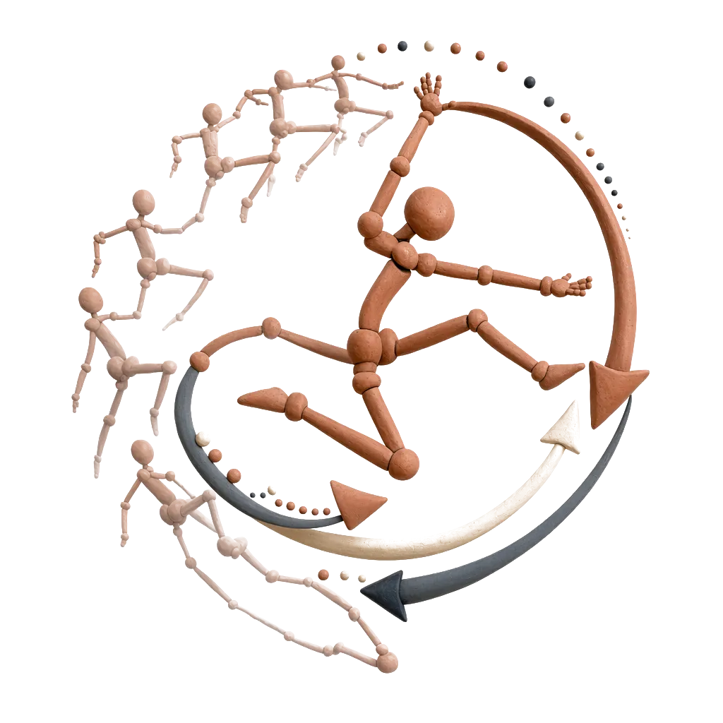
We apply semi- and weakly-supervised learning to human pose estimation, as illustrated in Figure 1. In our method with all functions proposed in this paper, fully-annotated images each of which has a pose annotation (i.e., skeleton) and an action label are used to acquire initial pose models for each action (e.g., “Baseball” and “Tennis” in Figure 1). These action-specific pose models are used to estimate candidate human poses in each action-annotated image. If a candidate pose is considered true-positive, the given pose with its image is used for re-learning the corresponding action-specific pose model.
The key contributions of this work are threefold:
True-positive poses are selected from candidate poses based on a pose feature representing the configuration of all body parts. This is in contrast to a pose estimation step in which only the pairwise configuration of neighboring/nearby parts is evaluated for efficiency.
- 2.
The action label of each training image is utilized for weakly-supervised learning. Because the variation of human poses in each action is smaller, pose estimation in each action works better than that in arbitrary poses.
- 3.
A large number of candidate poses are clustered by Dirichlet process mixtures for selecting true-positive poses based on the Bayes factor.
2 Related Work
A number of methods for human pose estimation employed (1) deformable part models (e.g., pictorial structure models [7]) for globally-optimizing an articulated human body and (2) discriminative learning for optimizing the parameters of the models [8]. In general, part connectivity in a deformable part model is defined by image-independent quadratic functions for efficient optimization via distance transform. Image-dependent functions (e.g., [9, 10]) disable distance transform but improve pose estimation accuracy. In [11], on the other hand, image-dependent but quadratic functions enable distance transform for representing the relative positions between neighboring parts.
While global optimality of the PSM is attractive, its ability to represent complex relations among parts and the expressive power of hand-crafted appearance feature are limited compared to deep neural networks. Recently, deep convolutional neural networks (DCNNs) improve human pose estimation as well as other computer vision tasks. While DCNNs are applicable to the PSM framework in order to represent the appearance of parts as proposed in [11], DCNN-based models can also model the distribution of body parts. For example, a DCNN can directly estimate the joint locations [12]. In [13], multi-resolution DCNNs are trained jointly with a Markov random field. Localization accuracy of this method [13] is improved by coarse and fine networks in [14]. Recent approaches explore sequential structured estimation to iteratively improve the joint locations [15, 16, 17, 18].
One of these methods, Convolutional pose machines [18], is extended to real-time pose estimation of multiple people [19] and hands [20]. Ensemble modeling can be also applied to DCNNs for human pose estimation [21]. Pose estimation using DCNNs is also extended to a variety of scenarios such as personalized pose estimation in videos [22] and 3D pose estimation with multiple views [23].
As well as DCNNs accepting image patches, DNNs using multi-modal features are applicable to human pose estimation; multi-modal features extracted from an estimated pose (e.g., relative positions between body parts) are fed into a DNN for refining the estimated pose [24].
While aforementioned advances improve pose estimation demonstrably, all of them require human pose annotations (i.e., skeletons annotated on an image) for supervised learning. Complexity in time-consuming pose annotation work leads to annotation errors by crowd sourcing, as described in [25]. For reducing the time-consuming annotations in supervised learning, semi- and weakly-supervised learning are widely used.
Semi-supervised learning allows us to utilize a huge number of non-annotated images for various recognition problems (e.g., human action recognition [26], human re-identification[27], and face and gait recognition [28]). In general, semi-supervised learning annotates the images automatically by employing several cues in/with the images; for example, temporal consistency in tracking [29], clustering [30], multimodal keywords [31], and domain adaptation [32].
For human pose estimation also, several semi-supervised learning methods have been proposed. However, these methods are designed for limited simpler problems. For example, in [33, 34], 3D pose models representing a limited variation of human pose sequences (e.g., only walking sequences) are trained by semi-supervised learning; in [33] and [34], GMM-based clustering and manifold regularization are employed for learning unlabeled data, respectively. For semi-supervised learning, not only a small number of annotated images but also a huge amount of synthetic images (e.g., CG images with automatic pose annotations) are also useful with transductive learning [35].
In weakly-supervised learning, only part of full annotations are given manually. In particular, annotations that can be easily annotated are given. For human activities, full annotations may include the pose, region, and attributes (e.g., ID, action class) of each person. Since it is easy to provide the attributes rather than the pose and region, such attributes are often given as weak annotations. For example, only an action label is given to each training sequence where the regions of a person (i.e. windows enclosing a human body) in frames are found automatically in [36]. Instead of the manually-given action label, scripts are employed as weak annotations in order to find correct action labels of several clips in video sequences in [37]; action clips are temporally localized. Not only in videos but also in still images, weak annotations can provide highly-contextual information. In [38], given an action label, a human window is spatially localized with an object used for this action. For human pose estimation, Boolean geometric relationships between body parts are used as weak labels in [39].
Whereas pose estimation using only action labels is more difficult than human window localization described above, it has been demonstrated that the action-specific property of a human pose is useful for pose estimation (e.g. latent modeling of dynamics [40, 41], switching dynamical models in videos [42], efficient particle distribution in multiple pose models in videos [43, 44], and pose model selection in still images [45]).
3 Human Pose Estimation Model
This section introduces two base models for human pose estimation, deformable part models and DCNN-based heatmap models.
3.1 Deformable Part Models
A deformable part model is an efficient model for articulated pose estimation [7, 8, 11]. A tree-based model is defined by a set of nodes, , and a set of links, , each of which connects two nodes. Each node corresponds to a body part and has pose parameters (e.g., 2D image coordinates, orientation, and scale), which localize the respective parts. Pose parameters are optimized by maximizing the given score function consisting of a unary term, S^{i}(\mbox{\boldmath{p}}_{i}) , and a pairwise term, P^{i,j}(\mbox{\boldmath{p}}_{i},\mbox{\boldmath{p}}_{j}), as follows:
[TABLE]
where \mbox{\boldmath{p}}_{i} and denote a set of pose parameters of the -th part and a set of \mbox{\boldmath{p}}_{i} of all parts (i.e. \mbox{\boldmath{P}}=\left\{\mbox{\boldmath{p}}_{1},\cdots,\mbox{\boldmath{p}}_{N^{(V)}}\right\}^{T}, where denotes the number of nodes), respectively. S^{i}(\mbox{\boldmath{p}}_{i}) is a similarity score of the -th part at \mbox{\boldmath{p}}_{i}. P^{i,j}(\mbox{\boldmath{p}}_{i},\mbox{\boldmath{p}}_{j}) is a spring-based function with a greater value if the relative configuration of pairwise parts, \mbox{\boldmath{p}}_{i} and \mbox{\boldmath{p}}_{j}, is probable.
In a discriminative training methodology proposed in [8], the parameters of functions S^{i}(\mbox{\boldmath{p}}_{i}) and P^{i,j}(\mbox{\boldmath{p}}_{i},\mbox{\boldmath{p}}_{j}) are trained with pose-annotated positive and negative training images.
3.2 DCNN-based Heatmap Models
Unlike deformable part models, recent DCNN-based human pose estimation methods (e.g., [46, 47, 48, 49, 50, 18, 51]) acquire the position of each body joint from its corresponding heatmap. The heatmap of each joint is outputted from a DCNN as shown in Figure 2. The position with the maximum likelihood in each heatmap is considered to be the joint position.
General DCNNs for human pose estimation consist of convolution, activation, and pooling layers. In order to capture local and spatially-contextual (e.g., kinematically-plausible) evidences for joint localization, smaller and wider convolutional filters are used, respectively. Further contexts are represented by sequential/iterative feedbacks of DCNN responses; see [18, 51, 17] for example. Figure 3 shows an example of heatmaps generated by iterative inference stages in [18], which was employed as a base model in our experiments.
4 Semi-supervised
Pose Model Learning by Correct-pose selection using Full-body Pose Features
Our semi-supervised pose model learning uses two training sets. The first set consists of images each of which has its human pose annotation and action label. Each image in the second set has no annotation. The first and second sets are called the fully-supervised (FS) and unsupervised (US) sets, respectively.
An initial pose model is learned from the FS set. This pose model is then used for the pose estimation of images in the US set. Note that a sole model is used in this section unlike the action-specific models of the complete scheme illustrated in Figure 1. All estimated poses must be classified into true-positives and false-positives to use only true-positives for re-learning the pose model.
Examples of false-positives are shown in Figure 4. Among various poses, some (e.g., (a), (b), and (c)) are evidently far from plausible human poses; e.g., the left and right limbs overlap unnaturally in (c). Such atypical poses are obtained by a human pose model described in Section 3, because this model optimizes more or less local regions in a full body. Despite the relative locations of local parts being plausible, the configuration of all parts might be implausible.
On the other hand, it is computationally possible to evaluate how plausible each optimized configuration of the parts is after the pose estimation process. In our semi-supervised learning, therefore, multiple poses are obtained from each training image in the US set by conventional pose estimation method(s) and evaluated whether or not each of them is plausible as the full-body configuration of a human body. With a DPM, multiple candidate poses are obtained with a loose threshold for score (1). With a DCNN-based model, all combinations of local maxima above loose thresholds in the heatmaps are regarded as candidate poses.
These candidate poses are evaluated to detect true-positive poses by the linear SVM. This correct-pose-selection SVM (CPS-SVM) is trained with the following two types of samples:
Positive:
Images and pose annotations in the FS set (Figure 5 (a)) are used as positive samples. To synthesize more samples, in each supervised training image, the end points of all limbs in the pose annotation are shifted randomly (Figure 5 (b)) 111While our proposed method shifts only limbs to accept subtle mismatches between an estimated pose and image cues, a more variety of positive samples can be synthesized by image deformation according to the shifted limbs [53]. within a predefined threshold, , of the PCP evaluation criterion [54, 53].
Negative:
Human pose estimation is applied to background images (Figure 5 (c)) with no human region. Detected false-positives (Figure 5 (d)) are used as negative samples.
From each pose in an image in the US set, the following two features are extracted and concatenated to be a pose representation (PR) feature for the CPS-SVM:
Configuration feature:
A PR feature should represent the configuration of all body parts to differentiate between different human poses. Such features have been proposed for action recognition [55, 56]. In the proposed method, the relational pose feature [55] that is modified for 2D - image coordinates is used. The 2D relational pose feature [56] consists of three components; distances between all the pairs of keypoints, orientations of the vector connecting two keypoints, and inner angles between two vectors connecting all the triples of keypoints. Given 14 full-body keypoints in our experiments, the number of these three components are , , and , respectively. In total, the relational pose feature is a 1274-D vector.
Appearance feature:
HOG features [57] are extracted from the windows of all parts and used for a PR feature.
The closest prior work to the CPS-SVM is presented in [58], which is designed for performance evaluation. This pose evaluation method features a marginal probability distribution for each part as well as image and geometric features extracted from a window enclosing the upper body. Rather than such features, the configuration feature (i.e., relative positions between body parts [55, 56]) is discriminative between different actions and so adopted in our PR feature; action-specific modeling is described in Section 5.
Instead of the CPS-SVM, a DNN is used in [24] for selecting true-positive poses. Whereas DNNs are potentially powerful and actually outperform SVM-based methods in recent pose estimation papers (e.g., [12, 15, 59, 13, 14]), they in general require a large number of training data for overfit avoidance. Since (1) our semi-supervised learning problem is assumed to have fewer supervised training data and (2) the PR feature is a high-dimensional data, the proposed method employs the SVM instead of DNNs.
Detected true-positive human poses in the US set are then used for re-learning a pose model with the FS set.
The aforementioned pose estimation, pose evaluation, and pose model re-learning phases can be repeated until no true-positive pose is newly detected from the US set.
In the first iteration, the pose estimation and evaluation phases are respectively executed with the pose model and the CPS-SVM that are trained by only the fully-supervised data. These pose model and the CPS-SVM are updated in the pose model re-learning phase and are used in the second or later iterations. All other settings are same in all iterations.
However, these phases were repeated only twice to avoid overfitting in experiments shown in this paper.
This semi-supervised learning allows us to only re-learn human poses similar to those in the FS set. In this sense, this learning scheme is based on the smoothness assumption for semi-supervised learning [60].
5 Semi- and Weakly-supervised
Pose Model Learning with Action-specific Pose Models
In this section, semi-supervised learning, proposed in Section 4, is extended with weakly-supervised learning. Each image in the weakly-supervised (WS) set is annotated with its action label. This WS set is used for our weakly-supervised learning instead of the US set.
The CPS-SVM proposed in the previous section is designed under the assumption that the observed configurations of body parts are limited. The possible configurations are more limited if the action of a target person is known. Figure 6 shows pose variations in athletics, badminton, and gymnastics, which are included in the LSP dataset [4]. It can be seen that the pose variation depends on the action. Based on this assumption, the proposed semi- and weakly-supervised learning generates action-specific pose models and CPS-SVMs. Since action-specific models are useful under the assumption of pose clusters depending on the action, the cluster assumption [60] is utilized in this learning scheme.
Initially, a general pose model is learned using all training images in the FS set. This initial model is then optimized for each action-specific model by using only its respective images in the FS set. For this optimization, in a DPM pose estimation model, the general model is used as an initial model in order to re-optimize the parameters of two functions S^{i}(\mbox{\boldmath{p}}_{i}) and P_{i,j}(\mbox{\boldmath{p}}_{i},\mbox{\boldmath{p}}_{j}) in Eq. (1) by using only the training images of each action. In a DCNN-based model, the general model is fine-tuned using the training images of each action.
The -th action-specific pose model is used to estimate candidate poses in images with the -th action label in the WS set. Each estimated pose is evaluated whether or not it is correct by the -th action-specific CPS-SVM. If the estimated pose is considered correct, this pose and its respective image are used for iterative re-learning of the -th action-specific pose model with the FS set, as with semi-supervised learning described in Section 4,
After the iterative re-learning scheme finishes, a pose model is learned from all actions’ images used in this re-learning (i.e., all images in the FS set and WS images in which correct human poses are selected).
6 Semi- and Weakly-supervised
Pose Model Learning with Outlier Detection by Clustering based on Dirichlet Process Mixtures
A key disadvantage of the learning schemes described in Sections 4 and 5 is that the CPS-SVM allows us to only extract human poses similar to those included in the FS set. In other words, it is difficult to re-learn poses whose 2D configurations of body parts are plausible but quite different from those in the FS set. The method proposed in this section extracts more true-positive poses based on the assumption that similar true-positives compose cluster(s) in the PR feature space of each action.
Let and denote the number of all candidate poses and their clusters, respectively. While is unknown, clustering with Dirichlet process mixtures [61], expressed in Eq. (2), or other non-parametric Bayesian clustering can estimate and assign the PR features of the candidate poses to the clusters simultaneously.
[TABLE]
where denotes a Dirichlet process with scaling factor and base distribution .
Clustering with Dirichlet process mixtures tends to produce clusters with fewer features [62, 63]. These small clusters are regarded as outliers with false-positive candidate poses and must be removed in our re-learning scheme. This outlier detection is achieved by [64], which evaluates the Bayes factor between an original set of clusters and its reduced set generated by merging small (outlier) clusters with other clusters. This method [64] is superior to similar methods because a Bayesian inference mechanism inference allows us to robustly find small outlier clusters rather than simple thresholding (e.g., [65]).
This outlier detection [64] is based on modified Dirichlet process mixtures, presented in Eq. (3). In Eq. (3), parameter set \mbox{\boldmath{\theta}}=\{\theta_{1},\cdots,\theta_{N^{(P)}}\} in Eq. (2) is decomposed into two parameters, and ; \mbox{\boldmath{\phi}}=\{\phi_{1},\cdots,\phi_{N^{(C)}}\} is the set of unique values in , and \mbox{\boldmath{z}}=\{z_{1},\cdots,z_{N^{(P)}}\} is the set of cluster membership variables such that if and only if . Note that the number of unique values, , is equal to the number of pose clusters defined above. If , features and are in the same cluster; \mbox{\boldmath{X}}=\{x_{1},\cdots,x_{N^{(P)}}\} is a set of all PR features of the candidate poses in this paper.
[TABLE]
where p(\mbox{\boldmath{z}}) is a prior mass function obtained by the Polya urn scheme [61]. is the gamma function taking the number of PR features in -th cluster (denoted by ). If , and are in the same cluster. This model is a type of product partition models [66].
For the outlier detection, first of all, an initial partition, \mbox{\boldmath{z}}_{I}, is obtained by clustering with Dirichlet process mixtures [67]. Let be the union of all partitions formed by any sequence of merge operations on clusters in \mbox{\boldmath{z}}_{I}. For practical use, is produced from \mbox{\boldmath{z}}_{I} by merging only small clusters having a few PR features.
The basic criterion of [64] for outlier detection from \mbox{\boldmath{z}}_{I} is the expense of model complexity of each partition in . Outliers can be detected by evaluating the evidence favoring a complex model over a simpler model with no or fewer outliers. The Bayes factor, which is used in a model selection problem, allows us to evaluate this criterion (e.g., [68]). Given PR features, the plausibilities of two models \mbox{\boldmath{z}}_{I} and \mbox{\boldmath{z}}_{m}\in\mathcal{M}_{I} are evaluated by the following Bayes factor :
[TABLE]
A lower bound of supporting \mbox{\boldmath{z}}_{I} rather than \mbox{\boldmath{z}}_{m} is obtained under the posterior condition and the prior mass function p(\mbox{\boldmath{z}})\propto\prod^{N^{(C)}}_{k=1}\alpha\Gamma(N^{(P)}_{k}) in Eq. (3):
[TABLE]
where is the number of clusters merged to arrive at \mbox{\boldmath{z}}_{m}. is the number of PR features in -th cluster of -th partition. In the proposed method, the number of PR features, and , in inequality (4) is weighted by score (1) of pose detection as follows:
[TABLE]
where denotes the normalized score of -th pose in -th cluster of -th partition; the scores are normalized linearly so that all of them are distributed between 0 and 1.
In inequality (4), the left-hand side is the Bayes factor, , which is computed for all possible partition pairs (i.e., \mbox{\boldmath{z}}_{I} and \mbox{\boldmath{z}}_{m}\in\mathcal{M}_{I}) by the method of Basu and Chib [69] in our proposed method. The lower bound of is defined with parameter given in Eq. (3). To determine , the scale provided by Kass and Raftery [70] gives us an intuitive interpretation. Given , only if \mbox{\boldmath{z}}_{I} satisfies inequality (4) for all \mbox{\boldmath{z}}_{m}\in\mathcal{M}_{I}, then each of merged small clusters in are detected as outliers.
In the proposed method, re-learning using the CPS-SVM is primarily repeated for updating pose models. Then the updated pose models are used for re-learning with clustering and outlier detection. This re-learning is repeated until no new training image emerges for re-learning. Note that all images in the WS set are used in the process of pose estimation and outlier detection in all iterations.
7 Experimental Results
7.1 Experimental Setting
The proposed method was evaluated with the publicly-available LSP, LSP extended [4] and MPII human pose [5] datasets. Images in the LSP dataset were collected from Flickr using eight action labels (i.e., text tags associated with each image), namely athletics, badminton, baseball, gymnastics, parkour, soccer, tennis, and volleyball. However, not only one but also a number of tags including erroneous ones are associated with each image. On the other hand, an action label is given to each image in the MPII dataset, but the action labels are more fine-grained (e.g., serve, smash, and receive in tennis) than the LSP. These incomplete and uneven annotations make it difficult to automatically give one semantically-valid action label to each image in the datasets.
For our experiments, therefore, action labels shared among the datasets were defined as follows; athletics, badminton, baseball, gymnastics222 The MPII has no action label related to “parkour”, and human poses in “parkour” are similar to those in “gymnastics”. So “parkour” is merged to “gymnastics” in the LSP in our experiments. , soccer, tennis, volleyball, and general. Whilst one of these eight labels was manually associated with each of 2000 images (1000 training images and 1000 test images) in the LSP dataset and 10000 images in the LSP extend dataset, several fine-grained action classes in the MPII dataset were merged to one of these eight classes333The activity IDs of the training data extracted from the MPII dataset are “61, 126, 156, 160, 241, 280, 307, 549, 640, 653, 913, 914, 983”, “643, 806”, “348, 353, 522, 585, 736”, “328, 927”, “334, 608, 931”, “130, 336, 439, 536, 538, 934”, “30, 196, 321, 674, 936, 975” for athletics, badminton, soccer, baseball, gymnastics, soccer, tennis, and volleyball, respectively. . Table 1 shows the number of training and test data of the eight action classes in each dataset.
For pose estimation, we used methods proposed in [11] and [18]. This is because [11] and [18] are one of state-of-the-arts using the PSM and the DCNN, respectively, as shown in Table 2. Each of the two methods [11, 18] obtained candidate poses by loose thresholding, as described in Section 4. More specifically, in [18], the candidate poses were generated from joint positions (i.e., local maxima in heatmaps) that were extracted not only in the final output but also in all iterative inference stages (e.g., Figure 3).
7.2 Quantitative Comparison
Table 2 shows quantitative evaluation results. Note that all methods except our proposed methods (i.e., (a) – (f), (j), (k), (o), (p), and (t) – (v)) are based on supervised learning. The parameters of our proposed methods (i.e., of PCP criterion for positive sample selection in the CPS-SVM and of the product partition model) were set as follows: , which was determined empirically, and , which was selected based on the scale of Kass and Raftery [70] so that false-positives are avoided as many as possible even with reduction of true-positives. For all of our proposed methods (i.e., (g) – (i), (l) – (n), (q) – (s), and (w) – (y)), the FS set consisted of 500 images in the LSP. Remaining 500 images in the LSP were used as the WS set. Additional WS sets collected from the LSP extended and the MPII were used in “(q) – (s)” and “(w) – (y)”. While “(q) – (s)” used only the LSP extended, both of the LSP extended and the MPII were used in “(w) – (y)”.
Note that it is impossible to compare the proposed methods (i.e., semi- and weakly-supervise learning) with supervised learning methods on a completely fair basis. Even if the same set of images is used, the amount of annotations is different between semi/weakly-supervised and fully-supervised learning schemes. In general, the upper limitation of expected accuracy in the proposed method is the result of its baseline, if training data used in the baseline is split into the FS and WS sets for the proposed method.
As shown in Table 2, Baseline–2 [11] is superior to Baseline–1 [18] in most joints. The same tendency is observed also between our proposed methods using Baseline–1 and Baseline–2. It can be also seen that, in all training datasets, the complete version of the proposed method (i.e., Ours-weakC) is the best among three variants of the proposed methods. In what follows, only Ours-weakC–2 is compared with related work.
Comparison between (k) Baseline–2 [18] and (n) Ours-weakC–2 is fair in terms of the amount of training images, while pose annotations in 500 images were not used in the proposed method. The proposed method is comparable with the baseline in all joints. Furthermore, (n) Ours-weakC–2 outperforms (j) Baseline–2 (HALF). This is a case where the amount of annotated data is equal between the baseline and the proposed method, while the proposed method also uses extra WS data (i.e., remaining 500 training images in the LSP).
In experiments with two other training sets (i.e., “LSP+LSPext” and “LSP+LSPext+MPII”), only the WS set increases while the FS set is unchanged from experiments with the LSP dataset. As expected, in these two experiments, difference in performance gets larger between the baseline and the proposed methods than in experiments with the LSP. However, we can see performance improvement in the proposed methods as the WS set increases; (n) 73.6 % (s) 79.5 % (y) 81.4 % in the mean accuracy.
7.3 Detailed Analysis
Effectiveness in Each Action
As discussed in Section 7.2, the mean performance gain in our semi- and weakly-supervised learning is smaller than that in supervised learning; in Ours-weakC–2 vs. in Baseline–2 on average. Here we investigate the performance gain in each action class rather than on average. Table 3 shows the PCK-2.0 score of each action class on the test set of the LSP dataset. We focus on the performance gains normalized by the number of training human poses of each action class (i.e., values within brackets); the number of human poses in each action class is shown in Table 1. A gap of the normalized performance gains between the baseline [18] and the proposed method (i.e., Ours-weakC–2 Gain [(j) (y)]) is smaller in “gym+parkour” and “general” classes than other classes. The performance gains in other classes are better because human poses are action-dependent and easy to be modeled while “gym+parkour” and “general” classes include a large variety of human poses; see Figure 6 to visually confirm the pose variations of “athletics” and “gymnastics”.
Even the best action-specific gain in Ours-weakC–2 (i.e., in “soccer”) is less than the mean gain of Baseline–2 (i.e., ). However, in contrast to the mean score of Ours-weakC–2 (i.e., ), the best action-specific gain is closer to the mean gain of Baseline–2. In addition, the best action-specific gain normalized by the number of training data (i.e., in “soccer”) is reasonable compared with the normalized mean gain in Baseline–2 (i.e., , where the number of training human poses in the LSP, LSPext, and MPII are 500, 10000, and 27945, respectively).
The results above validate that our proposed method works better in actions where a limited variety of human poses are observed.
Effectiveness of re-learning
The effectiveness of re-learning depends on the number of true-positives selected from the WS set. For our method using [11] with the 500 FS and 500 WS images in the LSP dataset, Figure 7 shows (1) the rate of images in which true-positive pose(s) are included in candidate poses (indicated by “Detected TP”) and (2) the rate of images in which true pose-positive(s) are correctly selected from candidate poses (indicated by “Selected TP”). In this evaluation, a candidate pose is considered true-positive if its all parts satisfy the PCP criterion [54, 53]. Note that the results shown in Figure 7 were measured after the iterative learning ended.
In Figure 7, it can be seen that only a few poses were selected in gymnastics even in “Ours-weakC”. This is natural because (1) the distribution of possible poses in gymnastics is wide relative to the number of its training images and (2) overlaps between two sparse distributions (i.e., poses observed in the FS and WS sets of gymnastics) may be small.
In other actions, on the other hand, the number of selected poses could be increased by “Ours-weak” and “Ours-weakC” in contrast to “Ours-semi”. The difference between the two rates (i.e., “Detected TP” and “Selected TP”) represents the number of true poses that can be selected correctly from a set of candidate poses. This is essentially equivalent to precision of the pose selection methods. In addition to precision, recall is also crucial because true poses should be selected as frequently as possible:
[TABLE]
where , , and denote respectively the numbers of all true poses in the WS set (i.e., the number of images in the WS set), candidate poses selected as true ones by pose selection methods, and all candidate poses detected from the WS set. Nmb(\mbox{\boldmath{P}}) is a function that counts the number of poses included in pose set . These precision and recall rates are shown in Figure 8. From the figure, it can be seen that the precision rates are significantly high in almost all cases. That is, most selected poses are true-positive. Compared with the precision rates, the recall rates are lower. That is, many false-negatives are not used for re-learning. This means that the proposed pose selection approaches and parameters were conservative so that only reliable poses are selected and used for re-learning.
Figure 9 shows the convergence histories of (g) Ours-semi–1, (h) Ours-weak–1, and (i) Ours-weakC–1, which are shown in Table 2. After a big improvement in the first iteration, the second one can also improve the score. It can be seen that the improvement is saturated in the second iteration. In the worst case, the score was decreased as shown in the third or later iterations of Ours-weakC–1. This is caused due to overfitting and false-positive samples:
The overfitting occurs when only similar samples are detected by the CPS-SVM and used for model re-learning. The iterative sample detections using newly-detected similar samples possibly lead to detecting only similar samples.
- 2.
If false-positives are detected by the CPS-SVM, the iterative detections using those false-positives may lead to detecting more false-positives.
Following the above results, iterations are repeated only twice in our experiments as described in Section 7.1.
Effect of Data Augmentation for CPS-SVM
The effect of parameter was examined with the test data of the LSP (Figure 10).
For simplicity, the results of only the complete learning scheme with the training data of “LSP” (i.e., (i) Ours-weakC–1 in Table 2) are shown.
Compared with the growth of detected and selected true-positive poses (indicated by blue and red lines, respectively, in the figure) with increasing , false-positives (indicated by a green line) increases significantly. This may cause the decrease in the accuracy of pose estimation (indicated by purple bars) at or above .
Distributions of Detected True-positives
For validating the effect of the semi- and weakly-supervised learning scheme for selecting true-positives, Figure 11 visualizes the distribution of PR features in Ours-weakC–1. While all true-positives selected by the CPS-SVM (indicated by green) are close to poses in the FS set (indicated by blue), several true-positives selected by clustering (indicated by red) are far from the FS set as expected.
More Unsupervised Data
For our proposed scheme, unsupervised (US) data for semi-supervised learning is much easier to be collected than weakly-supervised (WS) data. Here, the performance gain with more US set is investigated. For the US set, the COCO 2016 keypoint challenge dataset [75] was used while no pose annotations in this dataset were used for our experiments. In total, over 126K human poses in the COCO were added to the US set.
The results are shown in Table 4. Compared with the huge number of the US set, the performance gain is limited (i.e., ). The performance might be almost saturated because only human poses that are similar to those included in the FS set can be detected and used for model re-learning in our semi-supervised learning. For more investigation, weakly-supervised learning using such a huge training data is one of interesting future research directions while we need action labels in the WS set.
Qualitative Results
Several pose estimation results are shown in Figures 12 and 13. In both figures, Baseline–2 [18] and our-weakC–2 are trained by half of LSP and by LSP+LSPext+MPII, respectively; namely, the former and latter correspond to (j) and (y), respectively. In Figure 12, the results of all keypoints are improved and localized successfully by our method. In Figure 13, on the other hand, one or more keypoints are mislocalized by our method.
From the results in Figure 13, we can find several limitations of our proposed method. In (1), (2), and (3), a pitching motion is observed. While a large number of training data for this kind of motion is included in “baseball” class, body poses in this class are diversified (e.g., pitching, batting, running, fielding). That makes it difficult to model the pose variation in this class. This difficulty can be possibly suppressed by more fine-grained action grouping. While (4) and (5) are “parkour” and “general”, respectively, these poses are not similar to any training samples in their respective action class. In (6), overlapping people make pose estimation difficult. For this problem, a base algorithm should be designed for multi-people pose estimation (e.g., [74, 19]).
More Quantitative Comparison
Pose estimation accuracy was evaluated also with the test data of the MPII dataset (Table 5). For comparison, our semi- and weakly-supervised learning scheme with clustering using training images of “LSP+LSPext+MPII”, which is equal to (y) Ours-weakC–2 in Table 2, is evaluated because it is the best among all of our proposed schemes. Only half of training images in the MPII were used for the FS set in our method. While our method used a small amount of human pose annotations (i.e., 13.7K, 29K, and 40K annotations in our method, MPII, and “LSP+LSPext+MPII”, respectively), the effectiveness of semi- and weakly-supervised learning is validated in comparison between our method and the base method [18] using only half of training data in the MPII (i.e., 83.4% vs. 75.9 % in the mean, which are underlined in Table 5).
8 Concluding Remarks
We proposed semi- and weakly-supervised learning schemes for human pose estimation. While semi- and weakly-supervised learning schemes are widely used for object localization and recognition tasks, this paper demonstrated that such schemes are applicable to human pose estimation in still images. The proposed schemes extract correct poses from training images with no human pose annotations based on (1) pose discrimination on the basis of the configuration of all body parts, (2) action-specific models, and (3) clustering and outlier detection using Dirichlet process mixtures. These three functionalities allow the proposed semi- and weakly-supervised learning scheme to outperform its baselines using the same amount of human pose annotations.
Future work includes candidate pose synthesis and true-positive pose selection using generative adversarial nets [77], which can synthesize realistic data from training data. Since candidate pose synthesis and true-positive pose selection play important roles in our proposed method, further improvement of these schemes should be explored.
Experiments with more training data is also important. This investigates and reveals the properties of the proposed schemes; for example, (1) the relationship between the scale of the WS set and the estimation performance and (2) the positive/negative effects of true-positives/false-positives. While our weakly-supervised learning scheme needs an action label in each training image, unsupervised learning is more attractive for increasing the amount of training images. Automatic action labeling/recognition in training images allows us to extend our weakly-supervised learning to unsupervised learning.
References
- [1]
A. Krizhevsky, I. Sutskever, G. E. Hinton, Imagenet classification with deep convolutional neural networks, in: NIPS, 2012.
- [2]
Y. Taigman, M. Yang, M. Ranzato, L. Wolf, Deepface: Closing the gap to human-level performance in face verification, in: CVPR, 2014.
- [3]
D. Ramanan, Learning to parse images of articulated bodies, in: NIPS, 2006.
- [4]
S. Johnson, M. Everingham, Clustered pose and nonlinear appearance models for human pose estimation, in: BMVC, 2010.
- [5]
M. Andriluka, L. Pishchulin, P. V. Gehler, B. Schiele, 2d human pose estimation: New benchmark and state of the art analysis, in: CVPR, 2014.
- [6]
O. Russakovsky, J. Deng, H. Su, J. Krause, S. Satheesh, S. Ma, Z. Huang, A. Karpathy, A. Khosla, M. Bernstein, A. C. Berg, L. Fei-Fei, ImageNet Large Scale Visual Recognition Challenge (2014).
- [7]
P. F. Felzenszwalb, D. P. Huttenlocher, Pictorial structures for object recognition, International Journal of Computer Vision 61 (1) (2005) 55–79.
- [8]
P. F. Felzenszwalb, R. B. Girshick, D. A. McAllester, D. Ramanan, Object detection with discriminatively trained part-based models, IEEE Trans. Pattern Anal. Mach. Intell. 32 (9) (2010) 1627–1645.
- [9]
B. Sapp, A. Toshev, B. Taskar, Cascaded models for articulated pose estimation, in: ECCV, 2010.
- [10]
N. Ukita, Articulated pose estimation with parts connectivity using discriminative local oriented contours, in: CVPR, 2012.
- [11]
X. Chen, A. L. Yuille, Articulated pose estimation by a graphical model with image dependent pairwise relations, in: NIPS, 2014.
- [12]
A. Toshev, C. Szegedy, Deeppose: Human pose estimation via deep neural networks, in: CVPR, 2014.
- [13]
J. J. Tompson, A. Jain, Y. LeCun, C. Bregler, Joint training of a convolutional network and a graphical model for human pose estimation, in: NIPS, 2014.
- [14]
J. Tompson, R. Goroshin, A. Jain, Y. LeCun, C. Bregler, Efficient object localization using convolutional networks, in: CVPR, 2015.
- [15]
V. Ramakrishna, D. Munoz, M. Hebert, J. A. Bagnell, Y. Sheikh, Pose machines: Articulated pose estimation via inference machines, in: ECCV, 2014.
- [16]
S. Singh, D. Hoiem, D. A. Forsyth, Learning a sequential search for landmarks, in: CVPR.
- [17]
J. Carreira, P. Agrawal, K. Fragkiadaki, J. Malik, Human pose estimation with iterative error feedback, in: CVPR, 2016.
- [18]
S.-E. Wei, V. Ramakrishna, T. Kanade, Y. Sheikh, Convolutional pose machines, in: CVPR, 2016.
- [19]
Z. Cao, T. Simon, S.-E. Wei, Y. Sheikh, Realtime multi-person 2d pose estimation using part affinity fields, in: CVPR, 2017.
- [20]
T. Simon, H. Joo, I. Matthews, Y. Sheikh, Hand keypoint detection in single images using multiview bootstrapping, in: CVPR, 2017.
- [21]
Y. Kawana, N. Ukita, J. Huang, M. Yang, Ensemble convolutional neural networks for pose estimation, Computer Vision and Image Understanding 169 (2018) 62–74.
doi:10.1016/j.cviu.2017.12.005.
URL https://doi.org/10.1016/j.cviu.2017.12.005
- [22]
J. Charles, T. Pfister, D. R. Magee, D. C. Hogg, A. Zisserman, Personalizing human video pose estimation, in: CVPR, 2016.
- [23]
G. Pavlakos, X. Zhou, K. G. Derpanis, K. Daniilidis, Harvesting multiple views for marker-less 3D human pose annotations, in: CVPR, 2017.
- [24]
W. Ouyang, X. Chu, X. Wang, Multi-source deep learning for human pose estimation, in: CVPR, 2014.
- [25]
S. Johnson, M. Everingham, Learning effective human pose estimation from inaccurate annotation, in: CVPR, 2011.
- [26]
S. Jones, L. Shao, A multigraph representation for improved unsupervised/semi-supervised learning of human actions, in: CVPR, 2014.
- [27]
X. Liu, M. Song, D. Tao, X. Zhou, C. Chen, J. Bu, Semi-supervised coupled dictionary learning for person re-identification, in: CVPR, 2014.
- [28]
Y. Huang, D. Xu, F. Nie, Patch distribution compatible semisupervised dimension reduction for face and human gait recognition, IEEE Trans. Circuits Syst. Video Techn. 22 (3) (2012) 479–488.
- [29]
G. Li, L. Qin, Q. Huang, J. Pang, S. Jiang, Treat samples differently: Object tracking with semi-supervised online covboost, in: ICCV, 2011.
- [30]
A. Mahmood, A. S. Mian, R. A. Owens, Semi-supervised spectral clustering for image set classification, in: CVPR, 2014.
- [31]
M. Guillaumin, J. J. Verbeek, C. Schmid, Multimodal semi-supervised learning for image classification, in: CVPR, 2010.
- [32]
V. Jain, E. G. Learned-Miller, Online domain adaptation of a pre-trained cascade of classifiers, in: CVPR, 2011.
- [33]
R. Navaratnam, A. W. Fitzgibbon, R. Cipolla, Semi-supervised learning of joint density models for human pose estimation, in: BMVC, 2006.
- [34]
A. Kanaujia, C. Sminchisescu, D. N. Metaxas, Semi-supervised hierarchical models for 3d human pose reconstruction, in: CVPR, 2007.
- [35]
D. Tang, T. Yu, T. Kim, Real-time articulated hand pose estimation using semi-supervised transductive regression forests, in: ICCV, 2013.
- [36]
N. Shapovalova, A. Vahdat, K. Cannons, T. Lan, G. Mori, Similarity constrained latent support vector machine: An application to weakly supervised action classification, in: ECCV, 2012.
- [37]
O. Duchenne, I. Laptev, J. Sivic, F. Bach, J. Ponce, Automatic annotation of human actions in video, in: ICCV, 2009.
- [38]
A. Prest, C. Schmid, V. Ferrari, Weakly supervised learning of interactions between humans and objects, IEEE Trans. Pattern Anal. Mach. Intell. 34 (3) (2012) 601–614.
- [39]
G. Pons-Moll, D. J. Fleet, B. Rosenhahn, Posebits for monocular human pose estimation, in: CVPR, 2014.
- [40]
N. Ukita, M. Hirai, M. Kidode, Complex volume and pose tracking with probabilistic dynamical models and visual hull constraints, in: ICCV, 2009.
- [41]
N. Ukita, T. Kanade, Gaussian process motion graph models for smooth transitions among multiple actions, CVIU 116 (4) (2012) 500–509.
- [42]
J. Chen, M. Kim, Y. Wang, Q. Ji, Switching gaussian process dynamic models for simultaneous composite motion tracking and recognition, in: CVPR, 2009.
- [43]
J. Gall, A. Yao, L. J. V. Gool, 2d action recognition serves 3d human pose estimation, in: ECCV, 2010.
- [44]
N. Ukita, Simultaneous particle tracking in multi-action motion models with synthesized paths, Image Vision Comput. 31 (6-7) (2013) 448–459.
- [45]
N. Ukita, Iterative action and pose recognition using global-and-pose features and action-specific models, in: Workshop on Understanding Human Activities: Context and Interactions, 2013.
- [46]
A. Newell, K. Yang, J. Deng, Stacked hourglass networks for human pose estimation, in: ECCV, 2016.
- [47]
W. Yang, W. Ouyang, H. Li, X. Wang, End-to-end learning of deformable mixture of parts and deep convolutional neural networks for human pose estimation, in: CVPR, 2016.
- [48]
X. Chu, W. Ouyang, H. Li, X. Wang, Structured feature learning for pose estimation, in: CVPR, 2016.
- [49]
A. Bulat, G. Tzimiropoulos, Human pose estimation via convolutional part heatmap regression, in: ECCV, 2016.
- [50]
I. Lifshitz, E. Fetaya, S. Ullman, Human pose estimation using deep consensus voting, in: ECCV, 2016.
- [51]
T. Pfister, J. Charles, A. Zisserman, Flowing convnets for human pose estimation in videos, in: ICCV, 2015.
- [52]
Y. Yang, D. Ramanan, Articulated pose estimation with flexible mixtures-of-parts, in: CVPR, 2011.
- [53]
L. Pishchulin, A. Jain, M. Andriluka, T. Thormählen, B. Schiele, Articulated people detection and pose estimation: Reshaping the future, in: CVPR, 2012.
- [54]
V. Ferrari, M. J. Marín-Jiménez, A. Zisserman, Progressive search space reduction for human pose estimation, in: CVPR, 2008.
- [55]
A. Yao, J. Gall, L. J. V. Gool, Coupled action recognition and pose estimation from multiple views, International Journal of Computer Vision 100 (1) (2012) 16–37.
- [56]
H. Jhuang, J. Gall, S. Zuffi, C. Schmid, M. J. Black, Towards understanding action recognition, in: ICCV, 2013.
- [57]
N. Dalal, B. Triggs, Histograms of oriented gradients for human detection, in: CVPR, 2005.
- [58]
N. Jammalamadaka, A. Zisserman, M. Eichner, V. Ferrari, C. V. Jawahar, Has my algorithm succeeded? an evaluator for human pose estimators, in: ECCV, 2012.
- [59]
X. Fan, K. Zheng, Y. Lin, S. Wang, Combining local appearance and holistic view: Dual-source deep neural networks for human pose estimation, in: CVPR, 2015.
- [60]
O. Chapelle, B. Schölkopf, A. Zien, Semi-Supervised Learning, MIT Press, Cambridge, MA, USA, 2006.
- [61]
C. E. Antoniak, Mixtures of dirichlet processes with applications to bayesian nonparametric problems, Annals of Statistics 2 (6).
- [62]
J. W. Miller, M. T. Harrison, A simple example of dirichlet process mixture inconsistency for the number of components, in: NIPS, 2013.
- [63]
H. M. Wallach, S. Jensen, L. H. Dicker, K. A. Heller, An alternative prior process for nonparametric bayesian clustering, in: AISTATS, 2010.
- [64]
M. S. Shotwell, E. H. Slate, Bayesian outlier detection with dirichlet process mixtures, Bayesian Analysis 6 (4) (2011) 1–22.
- [65]
M. D. Escobar, M. West, Bayesian density estimation and inference using mixtures, Journal of the American Statistical Association 90 (430) (1995) 577–588.
- [66]
J. A. Hartigan, Partition models, Communications in Statistics, Theory and Methods 19 (9) 2745–2756.
- [67]
D. Aldous, Exchangeability and related topics, in: École d’Été St Flour 1983, Springer-Verlag, 1985, pp. 1–198, lecture Notes in Math. 1117.
- [68]
M. J. Bayarri, J. Morales, Bayesian measures of surprise for outlier detection, Journal of Statistical Planning and Inference 111 (1-2) (2003) 3–22.
- [69]
S. Basu, S. Chib, Marginal likelihood and bayes factors for dirichlet process mixture models, Journal of the American Statistical Association 98 (2003) 224–235.
- [70]
R. E. Kass, A. E. Raftery, Bayes factors, Journal of the American Statistical Association 90 (1995) 773–795.
- [71]
Y. Yang, D. Ramanan, Articulated human detection with flexible mixtures of parts, IEEE Trans. Pattern Anal. Mach. Intell. 35 (12) (2013) 2878–2890.
- [72]
X. Yu, F. Zhou, M. Chandraker, Deep deformation network for object landmark localization, in: ECCV, 2016.
- [73]
L. Pishchulin, E. Insafutdinov, S. Tang, B. Andres, M. Andriluka, P. Gehler, B. Schiele, Deepcut: Joint subset partition and labeling for multi person pose estimation, in: CVPR, 2016.
- [74]
E. Insafutdinov, L. Pishchulin, B. Andres, M. Andriluka, B. Schiele, Deepercut: A deeper, stronger, and faster multi-person pose estimation model, in: ECCV, 2016.
- [75]
T. Lin, M. Maire, S. J. Belongie, J. Hays, P. Perona, D. Ramanan, P. Dollár, C. L. Zitnick, Microsoft COCO: common objects in context, in: ECCV, 2014.
- [76]
G. Gkioxari, A. Toshev, N. Jaitly, Chained predictions using convolutional neural networks, in: ECCV, 2016.
- [77]
I. J. Goodfellow, J. Pouget-Abadie, M. Mirza, B. Xu, D. Warde-Farley, S. Ozair, A. C. Courville, Y. Bengio, Generative adversarial nets, in: NIPS, 2014.
The reference list from the paper itself. Each links out to its DOI / PubMed record.
- 1[1] A. Krizhevsky, I. Sutskever, G. E. Hinton, Imagenet classification with deep convolutional neural networks, in: NIPS, 2012.
- 2[2] Y. Taigman, M. Yang, M. Ranzato, L. Wolf, Deepface: Closing the gap to human-level performance in face verification, in: CVPR, 2014.
- 3[3] D. Ramanan, Learning to parse images of articulated bodies, in: NIPS, 2006.
- 4[4] S. Johnson, M. Everingham, Clustered pose and nonlinear appearance models for human pose estimation, in: BMVC, 2010.
- 5[5] M. Andriluka, L. Pishchulin, P. V. Gehler, B. Schiele, 2d human pose estimation: New benchmark and state of the art analysis, in: CVPR, 2014.
- 6[6] O. Russakovsky, J. Deng, H. Su, J. Krause, S. Satheesh, S. Ma, Z. Huang, A. Karpathy, A. Khosla, M. Bernstein, A. C. Berg, L. Fei-Fei, Image Net Large Scale Visual Recognition Challenge (2014). ar Xiv:ar Xiv:1409.0575 .
- 7[7] P. F. Felzenszwalb, D. P. Huttenlocher, Pictorial structures for object recognition, International Journal of Computer Vision 61 (1) (2005) 55–79.
- 8[8] P. F. Felzenszwalb, R. B. Girshick, D. A. Mc Allester, D. Ramanan, Object detection with discriminatively trained part-based models, IEEE Trans. Pattern Anal. Mach. Intell. 32 (9) (2010) 1627–1645.