Surface Fluctuating Hydrodynamics Methods for the Drift-Diffusion Dynamics of Particles and Microstructures within Curved Fluid Interfaces
David Rower, Misha Padidar, and Paul J. Atzberger

TL;DR
This paper develops fluctuating hydrodynamics methods for curved fluid interfaces to study particle dynamics, revealing unique power-law behaviors and providing theoretical explanations for surface-specific dissipation phenomena.
Contribution
It introduces novel surface fluctuating hydrodynamics approaches, including immersed boundary and stochastic Eulerian-Lagrangian methods, for curved interfaces with thermal fluctuations.
Findings
Power-law velocity autocorrelation scalings depend on geometry and viscosities.
Surface hydrodynamics differ from bulk fluid behavior, showing unique dissipation time-scales.
Methods successfully model passive particles and microswimmers on curved interfaces.
Abstract
We introduce fluctuating hydrodynamics approaches on surfaces for capturing the drift-diffusion dynamics of particles and microstructures immersed within curved fluid interfaces of spherical shape. We take into account the interfacial hydrodynamic coupling, traction coupling with the surrounding bulk fluid, and thermal fluctuations. For fluid-structure interactions, we introduce Immersed Boundary Methods (IBM) and related Stochastic Eulerian-Lagrangian Methods (SELM) for curved surfaces. We use these approaches to investigate the statistics of surface fluctuating hydrodynamics and microstructures. For velocity autocorrelations, we find characteristic power-law scalings , , and plateaus can emerge. This depends on the physical regime associated with the geometry, surface viscosity, and bulk viscosity. This differs from the characteristic scaling for…
Click any figure to enlarge with its caption.
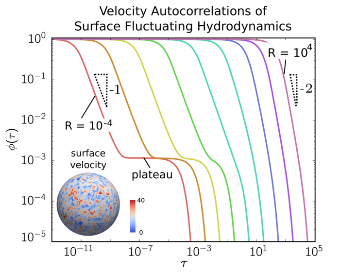 Figure 1
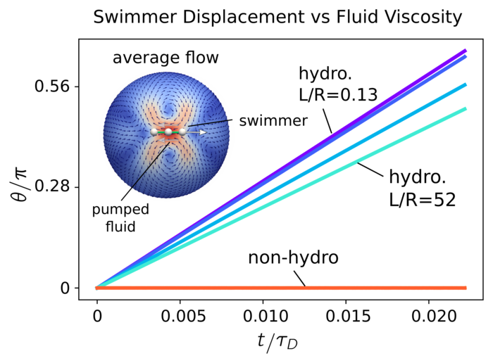 Figure 2
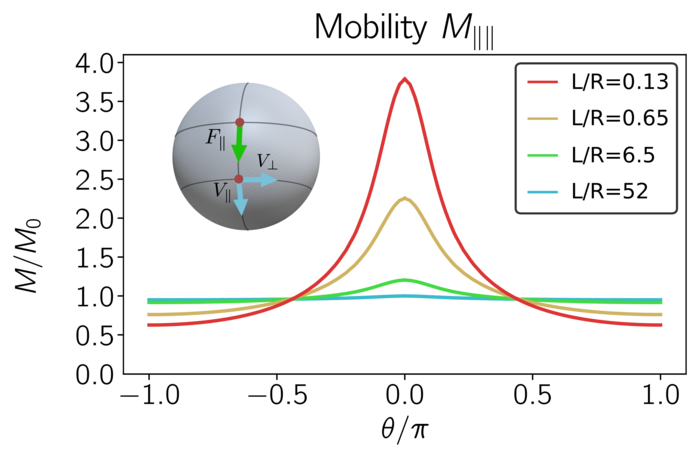 Figure 3
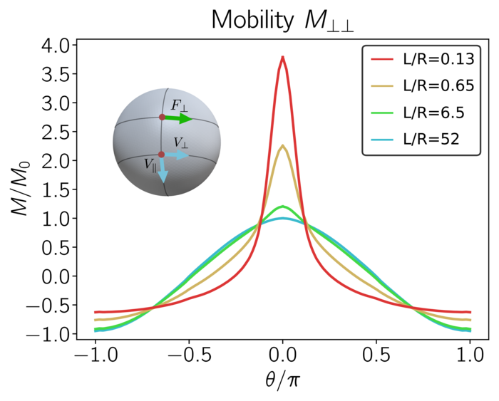 Figure 4
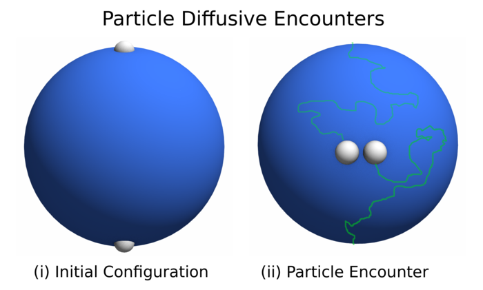 Figure 5
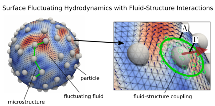 Figure 6
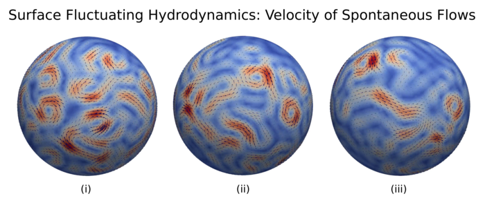 Figure 7
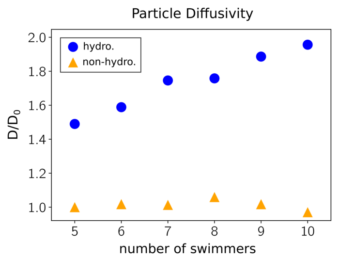 Figure 8
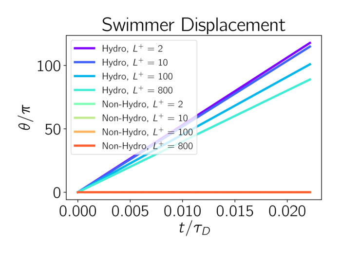 Figure 9
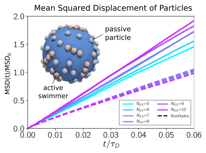 Figure 10
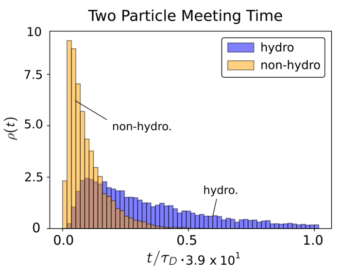 Figure 11
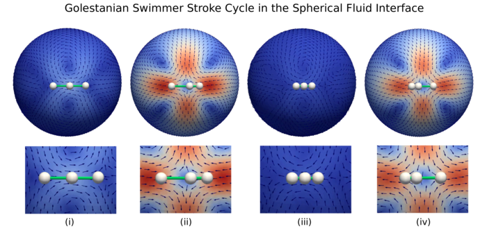 Figure 12
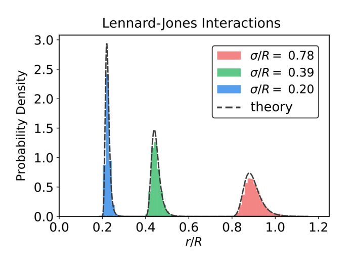 Figure 13
| Parameter | Value | Parameter | Value |
| 15.3 nm | 1.5 nm | ||
| 2.48 amu nm2 / ps | 3e-7 nm2/ps | ||
| 0.15 | |||
| 5e-6 | |||
| 100 |
| Variables | Values | Variables | Values |
| 15.3nm | 1.5nm | ||
| 2.48 amu nm2 / ps2 | 9.4577e-1 nm2 / ps | ||
| 5e-7 | |||
| 2.6222e-3 ps/amu | |||
| resI | 100 | I | 800 |
| 3 particles | |||
| 5 | 2 | ||
| 0 | |||
| 2 | |||
| 5e-3 |
| (hydro) | (hydro) | ||
| 0.13 | 1.167330 | 6.5 | 1.000000 |
| 0.65 | 1.138532 | 52 | 0.881074 |
Peer Reviews
No public reviews on file for this paper yet. If you reviewed it on a platform where reviews are public (OpenReview, ICLR, NeurIPS, ICML), you can paste yours below so the community can read it here.
Videos
No videos yet. Explain this paper in a talk, walkthrough, or lecture? Add one.
Taxonomy
TopicsLattice Boltzmann Simulation Studies · Heat and Mass Transfer in Porous Media · Surfactants and Colloidal Systems
Surface Fluctuating Hydrodynamics Methods for the Drift-Diffusion
Dynamics of Particles and Microstructures within Curved Fluid Interfaces
David A. Rower*∗*
Misha Padidar*∗*
and Paul J. Atzberger*∗*
W****e introduce fluctuating hydrodynamics approaches on surfaces for capturing the drift-diffusion dynamics of particles and microstructures immersed within curved fluid interfaces of spherical shape. We take into account the interfacial hydrodynamic coupling, traction coupling with the surrounding bulk fluid, and thermal fluctuations. For fluid-structure interactions, we introduce Immersed Boundary Methods (IBM) and related Stochastic Eulerian-Lagrangian Methods (SELM) for curved surfaces. We use these approaches to investigate the statistics of surface fluctuating hydrodynamics and microstructures. For velocity autocorrelations, we find characteristic power-law scalings , , and plateaus can emerge. This depends on the physical regime associated with the geometry, surface viscosity, and bulk viscosity. This differs from the characteristic scaling for bulk three dimensional fluids. We develop theory explaining these observed power-laws associated with time-scales for dissipation within the fluid interface and coupling to the surrounding fluid. We then use our introduced methods to investigate a few example systems and roles of hydrodynamic coupling and thermal fluctuations including for the kinetics of passive particles and active microswimmers in curved fluid interfaces.
1 Introduction
Soft materials can exhibit rich mechanical responses arising from curved fluid interfaces that mediate interactions between immersed particles and other microstructures [30, 43, 23]. This includes protein interactions within lipid bilayer membranes [2, 43, 73, 4], surfactants and contaminants in bubble interfaces [26, 84], transport in soap films [45, 47], and recent systems with nanoparticles or colloids embedded in fluid interfaces [17, 54, 90, 24, 89, 19, 14, 61]. Related hydrodynamic and curvature mediated phenomena also play an important role in biology and physiology, including transport of surfactants in lung alveoli [42, 57] or in cell mechanics [60, 63, 70]. We develop general approaches to model and simulate the collective drift-diffusion dynamics of particles and other microstructures embedded within curved two-dimensional fluid interfaces. At small length and time scales, our methods also allow for capturing the roles of fluctuations arising from active microstructures and from thermal effects [81, 76, 74, 14, 15].
We develop methods for curved surfaces building on our prior work on stochastic immersed boundary methods and fluctuating hydrodynamics methods [8, 9, 82]. We also draw on our recent work on developing approaches for deterministic incompressible hydrodynamic flows on curved surfaces [36, 37]. Here, we address how to introduce the spontaneous thermal fluctuations and handle the associated drift-diffusive dynamics of microstructures both for hydrodynamics in the inertial regime and the overdamped quasi-steady regime. We develop theory and computational methods that capture for the fluctuations the correlations arising from the hydrodynamic coupling within the curved fluid interface and from the traction stresses with the flows of surrounding bulk fluids.
Many past approaches for investigating hydrodynamic coupling and diffusion have been based on the classic Saffman-Delbrück (SD) hydrodynamics model [79, 78]. These were derived for flat viscous sheets [85, 55, 65, 16, 22, 66]. However, for many problems arising in practice, the geometry plays an important role as a consequence of significant curvature on the SD length-scale or from the surface topology. These effects can significantly change the hydrodynamic responses relative to the flat case [82, 75, 36, 43]. This has motivated recent work going beyond the classic Saffman-Delbrück theory to take into account the role of geometry and additional mechanical effects arising in curved fluid interfaces [41, 5, 75, 80, 24, 82, 36].
We introduce general fluctuating hydrodynamics methods for the drift-diffusion of particles and microstructures immersed within curved fluid interfaces. To demonstrate ideas, we focus particularly on the case of interfaces of spherical shape. To ensure finite diffusivities, as indicated in the SD theory, we formulate hydrodynamic equations for curved fluid interfaces coupled to surrounding bulk fluids. We introduce thermal fluctuations accounting for the fluid-structure interactions and collective dynamics of the particles and microstructures building on our prior work on stochastic immersed boundary methods and related approaches in [8, 9, 82, 36, 37].
For curved fluid interfaces, the geometry and topology pose additional challenges for developing stochastic immersed boundary methods and numerical approaches. This includes formulating and developing methods to solve hydrodynamic equations within curved surfaces and to obtain appropriate fluctuations and fluid-structure coupling operators [82]. We develop stochastic numerical methods and approaches for fluid-structure coupling operators taking the geometry into account. These numerical solvers and coupling operators allow us to obtain mobility tensors for the collective hydrodynamic coupling for modeling both passive and active microstructures within the interface.
The geometry and topology of curved interfaces also pose additional challenges for generating incompressible hydrodynamic fields and thermal fluctuations. We develop techniques to handle these aspects of the fluid mechanics based on formulating generalized vector potentials using the Hodge decomposition for manifolds. For the overdamped quasi-steady regime, we further develop techniques for the mobility tensor by using the embedding space to derive covariance structures that capture consistently hydrodynamic correlations in fluctuating fields. The embedding space expands the dimension of the problem and can create null-spaces for some of the linear operators. To address this issue, we develop algorithms based on stabilizations for computing the stochastic driving forces in the drift-diffusion dynamics of the microstructures. Our introduced approaches provide methods for both inertial and overdamped quasi-steady regimes. Our methods provide approaches for capturing in simulations the interface hydrodynamics, traction coupling with the surrounding bulk fluid, fluid-structure coupling, and thermal fluctuations.
We organize our paper as follows. We formulate the fluctuating hydrodynamic equations and related immersed boundary methods for spherical fluid interfaces in Section 2. Stochastic numerical methods for the drift-diffusion dynamics of microstructures are discussed in Section 3. We use our approaches to investigate the statistical mechanics of surface fluctuating hydrodynamics and to develop theory for explaining observed power-laws in Section 4. We further demonstrate our approaches by investigating the role of hydrodynamic coupling and related diffusive correlations in the kinetics of passive particles and active microswimmers in Section 4. The results show some of the rich phenomena that can arise for microstructures and fluctuating hydrodynamics within curved fluid interfaces.
2 Fluctuating Hydrodynamics for Curved Fluid Interfaces
To formulate the hydrodynamics of curved fluid interfaces, we will first develop the conservation laws with reference to the ambient embedding space. We will then develop descriptions in terms of operators that generalize the techniques of vector calculus used in continuum mechanics [59, 36].
2.1 Conservation Laws for Curved Surfaces
The conservation of mass and momentum of the fluid can be expressed as
[TABLE]
The and denote respectively the components of the fluid velocity normal and tangential to the fluid interface with . The denotes the local mean curvature of the surface [71]. The is the local mass density, the internal interfacial stress, and the body force per unit mass.
V The denotes the surface covariant divergence [1, 82, 36]. For a vector field represented as and , the surface covariant derivative gives , with . The and denotes the Christoffel symbols [1, 71]. The material derivative of the mass on a surface is , where is the local mean curvature. The material derivative of the momentum is [1, 36]. In the manifold setting, the material derivative of the vector field can be expressed as , where is the Lie derivative of under the flow of the velocity field [1, 59].
Throughout, we shall consider Newtonian incompressible fluid interfaces of fixed shape. In this case, the hydrodynamic flows are tangential to the surface. As a consequence, , , so that . For notational convenience, we suppress the and for the velocity and mass denoting them simply as and . The conservation laws simplify in this setting to
[TABLE]
The is now constant throughout and denotes the local force density. The stress tensor for an incompressible Newtonian fluid for a curved fluid interface can be expressed as
[TABLE]
The is the surface viscosity of the interfacial fluid, is the rate-of-deformation tensor, is the pressure, and is the metric associated identity tensor [59].
Tensors can be expressed in covariant or contravariant form [40, 1]. For vectors in contravariant form we have or in covariant form [1]. The denotes the coordinate basis vector. The denotes the coordinate basis covector (differential -form) with [1]. We can convert between vectors and covectors by the mappings and . The denotes the metric tensor and the inverse metric tensor [1]. The isomorphic maps and between the tangent space and cotangent space correspond operationally in calculations to lowering and raising indices in the coordinate expressions of the tensors [40, 1].
We find it convenient in our calculations to express tensors in covariant form and use exterior calculus [1]. This allows us to generalize vector calculus and many techniques employed for fluid mechanics to the manifold setting [36, 37, 82]. For an incompressible Newtonian fluid interface, the stress is given in equation 8. The divergence of the stress tensor on the surface becomes in covariant form [36, 82, 59]
[TABLE]
The is the local Gaussian curvature of the surface [71]. The is the exterior derivative playing a role similar to the gradient of the vector field on the surface. For a 1-form the exterior derivative is given by . The is the co-differential playing a role similar to the divergence on the surface [1]. The is the Hodge star which for a differential -form gives a complementary -form so that for any -form we have where is the volume form [1]. This also allows us to generalize vector calculus operators such as the curl and divergence to the surface by and . We give coordinate expressions for these operations and additional discussions in Appendix D
2.2 Fluctuating Hydrodynamics with Fluid-Structure Interactions
We develop surface fluctuating hydrodynamics descriptions to account for the drift-diffusion motions of microstructures and their hydrodynamic coupling within curved fluid interfaces [8, 9, 82]. In covariant form, we introduce for curved fluid interfaces fluctuating hydrodynamic equations incorporating fluid-structure interactions. We illustrate our general approach in Figure 1.
The fluid dynamics are modeled by
[TABLE]
The drift-diffusion motions of microstructures are modeled by
[TABLE]
The and denotes the collective configuration and velocity of the microstructures immersed within the fluid. The denotes the fluid velocity and the enforces the local incompressibility of the flow. The is the surface fluid shear viscosity, is the pressure, is the local Gaussian curvature, is the traction stress with the surrounding fluid. The are the conservative forces acting on the microstructures, and and are the stochastic forces accounting for thermal fluctuations of the system.
V The fluid-structure interactions result in two equal-and-opposite forces. The is a drag force of strength the microstructures experience from local coupling to the fluid. The is the opposite force density the fluid experiences locally from coupling to the microstructures. The is a spreading operator that serves to convert a local force to a local force density acting on the fluid. The is an averaging operator that serves to estimate a local reference velocity for a microstructure from the nearby fluid flow. We discuss specific choices for and in more detail in Section 2.5. V Given the rapid oscillations of the fluid from the thermal fluctuations, we neglect the advection terms which are expected to give lower-order contributions in equation 2.2 [86].
2.3 Traction Stress from Flow of the Surrounding Bulk Fluid
To obtain the traction stresses for the spherical geometry, we use Lamb’s solution [39, 49]. The traction arises from the surface flow with velocity entraining the surrounding bulk fluid [82]. Our approach makes the assumption that the bulk surrounding flow arises from an incompressible Newtonian fluid that reaches steady-state rapidly when contributing to the surface traction. Let the bulk fluid velocity be denoted by with values on the surface , where we shall assume throughout. The solution can be expressed using the spherical harmonics expansion
[TABLE]
We emphasize here the curl is the usual operator in three dimensional Euclidean space. The denotes the combined contributions of all of the solid spherical harmonic terms of degree . We also expand the bulk surrounding fluid flows inside the sphere and outside the sphere as
[TABLE]
The and are the solid spherical harmonic expansion terms combined for a given degree . The Lamb solutions for the bulk fluid velocity fields are given by [39, 49] expressible as
[TABLE]
where
[TABLE]
The traction stress expressed in contravariant form is
[TABLE]
The is the stress of the bulk surrounding fluid arising at the fluid interface. For the traction stress on the surface, note the is evaluated at the fixed location while . When taking the gradient the does not change, so that . We take throughout. The traction can be expressed in terms of the spherical harmonics expansion as
[TABLE]
The bulk fluid flow has on the fluid interface and is completely determined by . In covariant form, we define the traction operators on the surface corresponding to equation 21 and 22 as .
We remark that the approaches we develop can also be extended readily for surrounding fluids in systems that are subject to external shear flows or time-dependent flow responses. This would correspond to obtained from equations 19-20 being computed from stresses of such flows from other model hydrodynamic equations or results from numerical solvers [67, 43, 92, 24, 9]. For such surrounding fluids, with flows having time-dependence or flows having non-Newtonian responses, our approaches can also be used capture these dissipitative contributions to the mechanics and develop the associated thermal fluctuations [9, 86].
2.4 Thermal Fluctuations
To determine the associated stochastic driving terms and that account for thermal fluctuations, we use an approach related to our Stochastic Eulerian Lagrangian Method (SELM) framework [9, 86]. This gives and as Gaussian processes with -correlation in time, mean zero, and covariances
[TABLE]
The notation is to be interpreted as taking an expectation, . The equation 23 involves the dissipative operator associated with the fluid and is defined by
[TABLE]
The terms in equation 24 arise from the dissipative operator of the microstructure degrees of freedom and is defined by . The terms in equation 25 gives the cross-correlation that arises from microstructure-fluid coupling giving the operator and is defined by .
To express and generate efficiently the thermal fluctuations, it is useful to define a term . This term is taken to be independent of and to have covariance
[TABLE]
We can then express the thermal fluctuations for the hydrodynamics as . This gives the correlations in equations 23 – 25.
In our formulation, we use throughout that the fluid-structure coupling operators are adjoints , in the sense for all choices of and [82, 9]. We discuss choices for the coupling operators and the adjoint conditions in more detail in Section 2.5. For the stochastic driving terms of equations 2.2– 13 and 23– 25, our SELM approach ensures the Gibbs-Boltzmann distribution is invariant under the stochastic dynamics and satisfies detailed-balance [9, 86, 77]. The stochastic equations 2.2– 13 should be interpreted in the sense of Ito Calculus [64, 32].
We remark that the covariance operators in equations 23–25 are to be interpreted in the weak sense [56, 11, 9]. Consider and and and . The , , , are smooth fields and vectors playing the role of test functions. [56]. The associated covariances are
[TABLE]
The differential operator acts in the parameter . We also have the covariances
[TABLE]
and
[TABLE]
The operator acts in the parameter . Additional discussions on how to interpret these operator covariances also can be found in [11, 9].
2.5 Fluid-Structure Coupling: Immersed Boundary Methods for Curved
Surfaces
We handle the fluid-structure interactions between the microstructures with the fluid by developing extended immersed boundary methods in the manifold setting, see Figure 1, [69, 8, 9]. Many choices can be made for the operators and [9]. To ensure that the approximate fluid-structure coupling which converts between the Eulerian and Lagrangian reference frames are non-dissipative, the operators are taken to be adjoints [9, 69, 86].
We require the coupling operators satisfy the following adjoint conditions for any choice of test field and vector ,
[TABLE]
where the inner-products are defined as
[TABLE]
The denotes the collective vector of particle locations, or more abstract microstructure degrees of freedom [9]. For instance, the particle would be at location . The denotes the vector dot-product induced by the ambient physical space. For vector fields on the surface and we have . We use the notation to denote the adjoint condition 32.
In the setting of curved surfaces, the coupling operators and should be chosen carefully to control the velocity averaging and force spreading. The should ensure the velocity averaging takes into account over the surface the different tangential directions at each location. The for force densities should have well-controlled components for the surface in the tangential and normal directions. We develop operators of the form
[TABLE]
We use a tensor to sample and weight values on the surface to perform velocity averaging. We use the adjoint tensor to produce a corresponding force density field on the surface compatible with our adjoint conditions 32. For the curved surface, we use the geometrically motivated forms
[TABLE]
The sum runs over the indices of the particle or microstructure and the denotes the tangent basis vector in direction at location . We refer to the vector field as the probing vector field for direction .
On the sphere, the rotational symmetry can be utilized. For this case with the spherical coordinates , we take our probing vector fields to be of the form and , where . In practice, we truncate at length and use to normalize so that averages to one on the surface.
2.6 Overdamped Limit
In physical regimes with small Reynolds numbers , we consider the overdamped limit of the fluctuating hydrodynamic equations 2.2– 12 [9, 86]. In this regime, the limiting fluctuating hydrodynamic equations can be expressed as
[TABLE]
where
[TABLE]
This is obtained by taking the overdamped limit while retaining the finite slip term in equation 2.2 and 12. This results in the slip term in equation 40 [86]. In the strong-coupling limit with the mobility simplifies to
[TABLE]
The velocity averaging operator and force spreading operator are as discussed in Section 2.5. The denotes the solution operator for the hydrodynamic equations
[TABLE]
The gives the traction stresses with the surrounding bulk fluid as discussed in Section 2.2. The is the solution in the case with , where in practice we have .
To simply expressions, we also take for equation 39 the limit of no-slip between the microstructure and the fluid, which corresponds formally to . This yields throughout. Putting this together we arrive at the first term in equation 39. For the full stochastic system, we perform related detailed dimensional analysis and asymptotics in [9, 86, 82]. The equation 39 should be given the Ito interpretation. The thermal fluctuations involve configuration-dependent correlations resulting in the spontaneous drift term , [64, 32, 9, 86]. Additional analysis and reductions for different physical regimes can be found in [9, 86, 82].
2.7 Formulating Fluctuating Hydrodynamics on Surfaces using Vector
Potentials
The hydrodynamic responses both in the inertial fluctuating hydrodynamics of equation 2.2 and in the overdamped regime of equation 42 require computation of the operator of equation 27. Since the hydrodynamic fields are incompressible, we can use the Hodge decomposition of the fluid velocity . The and are vector potentials and is a harmonic function related to the topology of the manifold [59, 1]. The is the Hodge Laplacian and the is harmonic in the sense . For the case of spherical geometry with tangential velocity fields, we can express incompressible flows as , [82]. This uses that incompressibility requires and from the spherical geometry . This simplifies the action of the Hodge Laplacian and the representations. This allows for reformulating the inertial hydrodynamics of equation 2.2 in terms of as
[TABLE]
The denotes the contributions of the forces acting on the fluid. The denotes the Laplace-Beltrami operator [1]. The denotes the traction stress operator of equation 19 and 20. The denotes the operator in equation 27 for the hydrodynamic response.
We obtained equation 2.7 by substituting for , using , and using on both sides the generalized . We also use that the generalized curl commutes with the operator in the sense . The takes on a form similar to equation 27 but now applied to scalar fields. We provide more details for in terms of spherical harmonic coefficients below. These considerations allow for the fluctuating hydrodynamics to be expressed as
[TABLE]
In the overdamped regime, we need to compute the mobility tensor of the hydrodynamic coupling in equation 40. This requires us to solve the steady-state hydrodynamic equations 42. This can be reformulated as
[TABLE]
We again use that the generalized curl commutes with the operator in the sense . This yields for the steady-state hydrodynamics
[TABLE]
Central to both the inertial fluctuating hydrodynamics and steady-state regimes is computation of the action of the operator which gives the hydrodynamic responses of the system. We expand using spherical harmonics to represent the vector potential as where and denotes the spherical harmonics index, see Appendix C. For the spherical geometry, we can express solutions using that the spherical harmonics are eigenfunctions of the Laplace-Beltrami operator [82, 36].
The action of the operator can be expressed as
[TABLE]
where
[TABLE]
with . In the case with this can be simplified to
[TABLE]
where . We see from this that the hydrodynamic flow on the sphere is characterized by the non-dimensional parameter , where is the Saffman-Delbrück length-scale [79] and the radius of the sphere.
In the overdamped regime, to obtain the steady-state hydrodynamics, we can solve the hydrodynamic equations to obtain directly the spherical harmonics coefficients as
[TABLE]
For the inertial fluctuating hydrodynamics of equation 2.2 and equation 2.7, we can express the dynamics in terms of the spherical harmonics coefficients as
[TABLE]
where . The stochastic driving terms are associated with the hydrodynamics. These are complex-valued Gaussian processes -correlated in time with mean zero and covariance
[TABLE]
The stochastic driving terms are associated with the fluid-structure coupling discussed in Section 2.5. This involves the contributions from the dissipative terms in equation 2.2. The are complex-valued Gaussian processes having correlations with the microstructure stochastic dynamics in equation 12. We can express this as
[TABLE]
The gives the surface -inner product. The denotes the eigenvalue of the Laplace-Beltrami operator . The denotes the Kronecker -function which is zero for and one for .
The real-space fluctuating velocity field can be recovered using . This is derived from the stochastic force acting on microstructures in equation 12. Together, these stochastic driving terms give in real-space which satisfy equations 23–25.
In summary, the equations 2.7– 52 give a formulation for surface fluctuating hydrodynamics incorporating fluid-structure interactions in terms of the vector potential . The use of such Hodge decompositions and vector potentials is particularly convenient when representing velocity fields on surfaces. We give additional details on the derivation of these results in Appendix A.
3 Stochastic Numerical Methods
We develop numerical methods for the drift-diffusion dynamics of microstructures both in the inertial and overdamped regimes. To handle the incompressibility constraint for the surface hydrodynamics we make use of the generalized vector potential formulation discussed in Section 2.7.
3.1 Inertial Regime
In the inertial regime, we formulate the time-step integration of the fluctuating hydrodynamics of equation 2.2 in terms of stochastic dynamics of the vector potential in equation 2.7 and 2.7. We use a time-step update in terms of the spherical harmonics coefficients of given by
[TABLE]
For the microstructure dynamics, we use an update
[TABLE]
We have with the fluid velocity obtained by . Similarly, from the fluid-structure coupling we obtain the terms . The hydrodynamic time-step updates in equation 3.1 are related to the Euler-Maruyama method [46] and the microstructure updates in equation LABEL:eqn:verlet_update are related to modified velocity-verlet methods [88, 29, 38]. This gives in the stochastic setting errors with worse-case scalings , [88, 29, 38].
We account for thermal fluctuations of the microstructures over the time-step through the Gaussian term . This has mean zero and covariance
[TABLE]
The are complex-valued Gaussians with mean zero and covariance
[TABLE]
The are given by equation 48 or 2.7 and are the equilibrium fluctuations of the modes given by
[TABLE]
The are the eigenvalues of the Laplace-Beltrami operator on the surface. For the .
The are complex-valued Gaussians which we generate from by
[TABLE]
This ensures proper correlations in the system between the microstructure and the fluctuating hydrodynamics. We note that in our derivation of there were negative cross-correlations with the fluid which we capture in our numerical methods consistent with equation 25. These cross-correlations play the important role of ensuring momentum conservation. They account for the spontaneous fluctuations that exchange momentum back and forth between the fluid and microstructures.
The integrator approach we have introduced works well when the time-scales are comparable between the microstructure evolution and hydrodynamics. When there is a disparity in these time-scales, stiff stochastic numerical time-step integrators can also be developed using the vector potential formulation. For instance, we can develop exponential time-stepping approaches similar to our prior works [8, 93]. As an alternative, an asymptotic analysis of the stochastic dynamics of the fluid-structure system can also be performed as in [86]. This can be used to formulate equations in overdamped regimes and develop stochastic numerical methods [86].
3.2 Overdamped Regime
For the overdamped regime, we develop numerical methods for simulations based on stochastic variants of the velocity-verlet method [88, 29, 38]. We account for the thermal drift term in the stochastic dynamics using an approach related to methods in [21, 27]. We update the collective configuration of the particles or microstructures of the system using
[TABLE]
The thermal fluctuations have correlations generated by , where . The are standard Gaussian random variates with independent components having mean zero and variance one. The thermal drift is approximated by numerically estimating an average by . For the random variable , the denotes one of the independent samples. This provides a probabilistic estimator for the divergence. The random variables and satisfy . This gives
[TABLE]
This follows an approach related to [21, 27]. The validity follows readily by Taylor expanding in the variable [33].
The stochastic velocity-verlet scheme in equation 59 can be viewed in stages as follows. The gives the predictor part of the update of the configuration that is used to evaluate the force and mobility . The gives the corrector part for the update of the configuration which makes use of the predictor data and additional contributions from the thermal drift term.
3.2.1 Generating Stochastic Forces from the Mobility Tensor
During numerical time-step integration of the drift-diffusion dynamics by equation 59, we must generate the stochastic driving term . One way to do this is to determine from the mobility the square-root factor satisfying . Cholesky factorization methods can be used for symmetric positive definite matrices [87]. However, in the current formulation this present challenges given that the mobility tensor for the surface hydrodynamics is singular since it only depends on the tangential component of the force, see equation 2.7. Working only with the surface coordinates also presents challenges since there is no global coordinate chart for spherical topologies [82]. We instead work in the embedding space, but this results in a representation for the mobility tensor that is only positive semi-definite preventing direct use of the Cholesky factorization method.
We remedy this situation by adding a block diagonal tensor to our grand mobility tensor of equation 41. We do this in a way that preserves the drift-diffusion dynamics in the tangential directions. This is accomplished by using rank-one stabilizations to obtain modified self-mobility blocks of the form . The is any chosen positive weight. The denotes the normal vector on the sphere at the location of . By using this modification, we can obtain a tensor that is positive definite. This allows us to use Cholesky factorizations to obtain satisfying .
Our introduced stabilizations are constructed orthogonal to the tangent directions of the surface. As a result, this only modifies the mobility responses in the directions normal to the surface and preserves the microstructure drift-diffusion dynamics in the tangential directions. We generate the tangential stochastic forces using , where . The are Gaussian vectors with independent components having mean zero and variance one. The denotes projection of the stochastic vector to the tangent space of the surface. This allows us to generate the stochastic terms for the thermal fluctuations in the surface drift-diffusion dynamics of the microstructures.
3.3 Computing Hydrodynamic Forces and Responses
To solve for the fluid velocity, we represent the force density term as with expansion . We compute this in practice by using the spherical harmonics representation of obtained by . The gives the representation of the force density in the ambient physical space with coordinates . The inner-products are approximated numerically by using Lebedev quadrature [53, 52]. We then compute . This uses the finite spherical harmonics expansion of , where denotes the term of the expansion associated with index . We compute using , where the inner-product is approximated numerically using Lebedev quadrature [53, 52]. From the solution coefficients , we obtain the fluid velocity on the surface from .
In practice, we numerically approximate inner-products by using Lebedev quadratures on the spherical surface [53, 52, 82]. We use , where denotes the quadrature computed inner-product with the weights and the nodes [53, 52, 82]. This provides a finite spherical harmonics expansion of . While other quadrature approaches could be used such as latitude and longitude sampling, the Lebedev quadrature nodes have octahedral symmetry and provide a better distribution of sampling nodes on the spherical surface [36, 82].
We remark that for the hydrodynamics on the sphere most of the representation of the flow responses and evolution is represented analytically using the spherical harmonics expansions. As a result, in the developed numerical methods the primary source of errors is from the truncation of the spherical harmonics expansion and related projections. In these methods, the primary source of computational expense arises from computing the -inner products using the quadratures and in summing the spherical harmonics expansions in reconstructions.
When using modes, this part of the numerical algorithms have a computational complexity of . In the inertial regime, the thermal fluctuations requires initially a single off-line computation of the Cholesky factorization of the covariance which costs . Generating the correlated variates then costs each time-step. In the overdamped case, the primary additional computational expense is from the Cholesky factorization of the mobility tensor. For microstructure degrees of freedom and modes, the overdamped case has computational complexity .
The Lebedev quadratures allow for computing the -inner products to a high level of accuracy. Available Lebedev quadratures allow for inner-products for functions expanded up to degree spherical harmonics to be computed up to round-off errors [52]. We performed convergence analysis of our spectral numerical methods using Lebedev quadratures for approximating exterior calculus operators and solving hydrodynamic equations in [35, 36].
4 Applications
We discuss a few applications showing how to use our introduced fluctuating hydrodynamics methods for investigating phenomena within curved fluid interfaces. We first discuss the hydrodynamic relaxation of fluctuating fluids and characterize scalings of the velocity autocorrelations. We find different scalings can emerge depending on the physical regimes associated with the interface geometry, surface viscosity, and bulk viscosity. We further investigate the mobilities associated with microstructures embedded within fluid interfaces in the quasi-steady regime. We then demonstrate the computational methods by studying the correlated diffusion of passive particles and the drift-diffusion dynamics of active microswimmers. The results show some of the rich phenomena within curved fluid interfaces that can arise from hydrodynamic coupling, thermal fluctuations, and geometry that our methods can be used to investigate.
4.1 Autocorrelations of the Surface Fluctuating Hydrodynamics
We investigate the autocorrelation of the fluid velocity of interfacial fluctuating hydrodynamics introduced in equation 2.2. We find the velocity autocorrelations can exhibit power-law decay with scalings and depending on the physical regime. We also find in some regimes a plateau behavior can arise. This differs from bulk three dimensional fluctuating hydrodynamics that would exhibit power-law decay. This also differs from purely two dimensional fluctuating hydrodynamics that would exhibit only a power-law decay [7, 8].
Interfacial fluctuating hydrodynamics involves both dissipation from the propagation of shearing motions within the interfacial fluid surface and from traction coupling with the bulk surrounding fluid. This results in two important time-scales. The first is the time-scale for shear stresses to propagate over the entire spherical surface . The second is the time-scale on which rigid-body rotation of the entire spherical interface dissipates energy significantly to the bulk surrounding fluid .
We explore these contributions to the velocity autocorrelations by varying the ratio . This involves the sphere radius and the Saffman-Delbrück length . We show our results in Figure 3. We take as default parameter values , , , , , and . We give details on our derivations analyzing these autocorrelations in Appendix B.
The velocity autocorrelations of the surface fluctuating hydrodynamics can be expressed using the following expansion in spherical harmonics
[TABLE]
The denotes the -directional component of the velocity and the denotes the spherical harmonic with mode . The metric factor on the sphere is . We also use that the velocity is isotropic and that and , where is given in equation 48. We derive scaling laws for different physical regimes using equation 61. We remark that all of our results use a truncated expansion with modes up to degree . This introduces a regularization length-scale similar to our immersed boundary coupling approaches for determining responses of particles and microstructures. Details of our derivations can be found in Appendix B.
When , we find the velocity correlations exhibit an initial decay to a power-law regime with scaling on time-scales . This is followed by a plateau regime that persists from . This eventually gives way to exponential decay for . The initial power law decay is associated with the propagation of shear stresses over the interface with negligible dissipation to the bulk. This persists until time-scale , see Figure 3.
We remark that this is similar to the velocity autocorrelations that would be observed in a purely two dimensional viscous Newtonian fluid, which can be computed readily using the methods in [7]. In contrast, for the spherical fluid interface the two dimensional fluid has finite area. This results in finite size effects in the flow responses and correlations.
A plateau arises in the case when which creates an intermediate regime. In the intermediate plateau regime, the shear stress has already propagated to the entire surface, but the dissipation into the bulk fluid of the rigid-body rotational motion has not yet become significant. On time-scales , the dissipation into the bulk fluid dominates through the rotational motions and gives exponential decay. As the increases, the plateau regime disappears when , as seen when moving left to right in Figure 3.
In the regime, the time-scales for decay from intra-interface shearing motions becomes reversed and large relative to the time-scale for decay from the coupling to the bulk fluid . This results in a new regime with power law scaling for time-scales . When this again eventually gives exponential decay from the rotational motions of the entire interface. The arises from simultaneous dissipation from the shearing motions within the interface and dissipation from coupling to the bulk fluid. We give more details and derivations of these power-laws and related time-scales in Appendix B.
4.2 Mobility Tensor for Interacting Particles and Microstructures
We compute numerically the mobility using equation 41. We obtain a numerical solver for the fluid velocity with force distribution on the spherical surface using equation 2.7 and Lebedev quadratures [53, 52, 82]. We performed convergence analysis of the numerical methods based on Lebedev spectral approaches in [35, 36].
From the symmetry of the sphere the mobility of particles can be determined from the canonical two particle mobility tensor. The two particle mobility obtained from equation 41 can be expressed as
[TABLE]
with
[TABLE]
The where we use notation and . The denote the self-mobilities and can be computed numerically once and stored.
The give for a force on the first particle the velocity response at the second particle. We can express this as , where for the two particle displacement we split into the parallel and perpendicular components. The and . Using the symmetry of the sphere we can tabulate numerically the two particle mobility tensor by using a canonical configuration of the two particles. We rotate the sphere so that the first particle is always situated at the north pole. We then align the geodesic displacement between the two particles in the -plane with tangent along the positive -axis. We denote the rotation operation by that moves any two particles into this canonical configuration . We can convert our canonical tabulated two-particle mobilities to the specific mobility of two particles by . We obtain the grand-mobility tensor for interacting particles by summing over all pairs of particles the two particle mobility tensors. We show the components of the two-particle mobility when in Figure 4 and 5.
4.3 Equilibrium Fluctuations
We validate our stochastic numerical methods by studying the drift-diffusion dynamics of interacting particles. A strong indication of the validity the methods is provided by consider how particles diffuse over time when subject to a conservative force. This requires the stochastic methods to capture both the drift dynamics accurately while also handling appropriately the thermal fluctuations of the system. From equilibrium statistical mechanics a configuration should have a probability distribution of the Gibbs-Boltzmann form [77, 18]
[TABLE]
The denotes the partition function and denotes the thermal energy of the system [77].
We consider the drift-diffusion dynamics of two hydrodynamically coupled particles having the non-linear Lennard-Jones interaction
[TABLE]
The denotes the distance between the two particles. The denotes the length-scale characterizing the radius of the particles. We find our stochastic numerical methods provide for the drift-diffusion dynamics very good agreement with the distribution predicted from equilibrium statistics mechanics from equation 68. We show these results for a few choices of in Figure 6.
For parameters, we take throughout the thermal energy amunm2/ps2, the strength of the potential , viscosity ratio . We use for the stochastic integrator in equation 59 the time-steps ps and drift estimator , .
4.4 Hydrodynamic Correlations in Particle Diffusion
Motivated by proteins in lipid bilayer membranes and recent results for synthetic colloidal systems [20, 31, 17, 61], we consider diffusion limited interactions by particles that interact within a curved fluid interface. We investigate the case with and without hydrodynamic coupling on the collective diffusivity and how this influences the time for particles to come into near contact.
We consider two particles initially at antipodal locations on the sphere (north and south pole) and the amount of time it takes for them to come into contact with each other. We consider the distribution for this meeting time in the case of hydrodynamic coupling with mobility as in Section 4.1 and in the case without hydrodynamics with a local drag having mobility response . We report these results with and without hydrodynamic interactions in Figure 8. We use in our studies the parameter values in Table 1.
The gives the radius of the spherical fluid interface, the gives the effective size of the particles used to specify the radius of separation for considering contacts, is the particle diffusivity, and is the slip permitted between the particle and the local fluid. The gives the Saffman-Delbrück lengths between the surface fluid viscosity and the surrounding bulk fluid viscosity inside and outside the spherical fluid interface. The gives the thermal energy.
We find in both cases that the meeting times remain on average on the same order of magnitude. However, the hydrodynamic coupling introduces significantly more variation in the meeting-time distribution producing a long-tail, see Figure 8. For systems where diffusive kinetics are important, we see the hydrodynamic coupling can significantly influence the distribution of encounters between particles.
4.5 Microscopic Swimmers and Mixing
We investigate hydrodynamic transport and diffusive mixing associated with swimmers at microscopic scales. Behaviors both individually and collectively can differ significantly from macroscopic scales [51, 72]. Swimming in both Newtonian and Non-Newtonian bulk fluids in three dimensional volumes have been investigated in [51, 72, 62]. We investigate here the case of swimmers within two dimensional curved fluid interfaces treated as a Newtonian fluid. Our approaches also could be used to study non-Newtonian fluids either by incorporating explicitly the microstructures in the fluid using approaches of Section 2.5 and [10], or by extending the formulation of the hydrodynamic equations to other constitutive laws in Section 2.1.
As a demonstration of the methods, we consider Golestanian Swimmers [62] that consist of three beads that interact through two oscillating harmonic bonds. The harmonic bonds have time-dependent rest-lengths with energy
[TABLE]
where . The bond lengths are offset in time to have different phases for and . To impose excluded volume, both the beads of the microscopic swimmers and the passive particles also interact through the Weeks-Chandler-Andersen (WCA) potential [91]
[TABLE]
The separation distance is denoted by for two particles and . The potential gives an effective particle steric radius of . We give parameters for our model in Table 2. We remark that this parameterization is for illustrative purposes of the methods and to obtain more physically realizable systems may require further adjustments.
The phase differences in the swimming strokes are crucial to break symmetry in time to have the possibility of a net forward motion. For steady-state hydrodynamics, a time-reversible motion would have no net displacement by the Scallop Theorem [72, 50, 44]. We also emphasize that without hydrodynamic coupling between the beads the swimmer would remain stationary. This is a consequence of the equal-and-opposite forces that act on the beads and average out to zero over the periodic strokes. Without the surrounding fluid, such forces can not move the center-of-mass of the swimmer.
The swimmer strokes generate flows that on average pump the fluid. We show the associated stages of the stroke cycle captured by our methods in Figure 9. The hydrodynamics is confined to a surface of spherical topology which results in flows with vortices. We show the average flow that pumps the fluid in the inset of Figure 10.
We study first how the swimmer’s speed depends on the viscosities of the two dimensional interfacial fluid and surrounding bulk fluid. We characterize the viscosities by the ratio of the Saffman-Delbrück length to the sphere radius as discussed in Section 2.7. We can consider the swimmer’s angular progression over the sphere from which the swimming speed can be estimated, see Figure 10. As the viscosity ratio increases, the generated flows transition from being relatively localized to enveloping most of the sphere. We find as the viscosity ratio increases from to that the swimming speed drops by approximately , see Table 3.
We next investigate the collective drift-diffusion dynamics of passive particles when subjected to mixing by multiple microscopic swimmers . Both the swimmers and particles are subjected to the hydrodynamic coupling and thermal fluctuations using the approaches we introduced in Section 2. We study as the number of microscopic swimmers increases how the effective diffusivity of the passive tracer particles is influenced.
We characterize the diffusivity by the Mean Squared Displacement (MSD)
[TABLE]
In the spherical geometry the standard Euclidean distance is distorted by the spherical surface. We use as our norm the geodesic distance on the surface between the starting point and the final point . Unlike bulk three dimensional fluids, the distance between points remains bounded since the surface is a compact manifold. As a consequence, we have that eventually the asymptotes to a limiting value. This corresponds to sampling the from the stationary distribution over the surface.
To estimate in practice the diffusivity, we consider the over time-scales with where is the time-scale to diffuse the distance . We find the is approximately linear in this regime and we characterize the passive particle motions by the diffusivity , see Figure 12. In practice, we estimate using the slope of the obtained from a least-squares fit to the data in the range .
We study how the diffusivity of passive tracer particles are enhanced by the action of swimmers. Both the passive tracers and swimmers undergo the drift-diffusive dynamics of equation 39 with parameters in Table 2. We remark there are some technical challenges in parameterizing consistently for comparisons the non-hydrodynamic and hydrodynamic dynamics. We choose to do this by using the diagonal entry of our mobility tensor as the inverse drag for the non-hydrodynamic dynamics. Given symmetries that can arise readily for small numbers of swimmers, we consider cases with .
Our initial studies reported here find the swimmers can result in significant enhancement of the tracer diffusivity relative to the non-hydrodynamic case, see Figure 12. In the case with no swimmers , we have diffusivity with hydrodynamic coupling and without hydrodynamic coupling . This has the ratio . We see already in the absence of any swimmers an effective enhancement of in the diffusivity of the particles from the hydrodynamic correlations.
As we introduce more microscopic swimmers , their collective stroke cycles contribute hydrodynamic flows that mix the tracer particles in addition to the thermal fluctuations. Relative to the non-hydrodynamic case, we find this manifests as an effective diffusivity that is further enhanced in the range of , see Figure 12. The thermal fluctuations allow for the tracer particles to diffuse between streamlines of the hydrodynamic flows that are transiently generated by the swimmers. The swimmers also can have their own motions driven by the mutual flows and thermal fluctuations that serve both to move their center-of-mass and to rotate their orientation. This combination of effects shows the interplay that can arise between hydrodynamically driven drifts and thermal fluctuations.
The results illustrate some of the hydrodynamic and thermal effects that can be captured using our methods for possible further investigations of passive and active soft materials [58, 81] or mechanics in cell biology [13, 60]. The introduced surface fluctuating hydrodynamics methods can be used to model passive and active spatially extended microstructures to capture both the hydrodynamic coupling and the correlated thermal fluctuations within curved fluid interfaces.
5 Conclusions
We have introduced surface fluctuating hydrodynamics approaches for general investigations of the drift-diffusion dynamics of particles and microstructures immersed within curved fluid interfaces. We introduced computational methods for simulations of fluid-structure interactions and collective dynamics driven by active forces and thermal fluctuations. We studied the velocity autocorrelations for surface fluctuating hydrodynamics in spherical geometries. We found for interfacial fluids there are different scalings that emerge for different physical regimes and depending on the interface geometry, surface viscosity, and bulk viscosities. We also showed how our methods can be used for modeling and simulating the collective drift-diffusion dynamics of both passive and active microstructures. We obtained results investigating the enhanced mixing of particles from active microswimmers. The results show how the introduced surface fluctuating hydrodynamics approaches can be used for investigating some of the rich phenomena that can arise in curved fluid interfaces.
6 Acknowledgments
The authors P.J.A, M.P. and D.A.R. acknowledge support from research grants DOE Grant ASCR PHILMS DE-SC0019246 and NSF Grant DMS - 1616353. We also acknowledge UCSB Center for Scientific Computing NSF MRSEC (DMR-1121053) and UCSB MRL NSF CNS-0960316. P.J.A. would also like to acknowledge a hardware grant from Nvidia.
Appendix A Derivations for Fluctuating Hydrodynamics on Surfaces using Vector
Potentials
We discuss in more detail for fluctuating hydrodynamics on the surface derivation of the stochastic dynamics of the vector potential . We express the dynamics in terms of complex-valued coefficients of a spherical harmonics expansion as
[TABLE]
The force expansion terms are obtained from the real-space force using equation 2.7. We obtain the stochastic driving fields and using a fluctuation-dissipation approach for the discretized system in a manner similar to our prior work [8, 9]. We generate Gaussian driving terms with mean zero and covariance
[TABLE]
This requires determination of the covariance for the equilibrium fluctuations of the modes .
The Gibbs-Boltzmann distribution for the equilibrium fluctuations depends on the kinetic energy of the fluid given by
[TABLE]
The where is the degree and the order. We used here the adjoint property of the co-differential and the exterior derivative [1]. The spherical harmonics modes have -norm given by and are eigenfunctions of the Laplace-Beltrami operator with eigenvalues .
The quadratic form of the energy yields that the equilibrium fluctuations of the spherical harmonics coefficients are Gaussian with mean zero and covariance
[TABLE]
The denotes the Kronecker -function where we use notation to denote the conjugate mode index. The spherical harmonics coefficients are complex-valued and the field must be real-valued. This requires for the coefficients .
We generate the stochastic driving terms using with and throughout. From the conditions in equation 74, we have for that
[TABLE]
As a consequence, we must have that and . This requires that . The case with is special since the mode is self-conjugate requiring
[TABLE]
As a consequence, we must have that and .
Algorithmically, for modes these results correspond to generating for by computing each of the components and as independent Gaussian random variates each having the covariance , and for setting . The modes with are special since they are self-conjugate and we have with covariance .
Appendix B Derivation of Power-Laws for Fluctuating Hydrodynamics on a Sphere
We find the autocorrelation of the fluid velocity on the spherical interface has significantly different behaviors than bulk fluids. For bulk Newtonian fluids occupying a three dimensional volume the velocity autocorrelation function has a well-known characteristic long-tail with scaling . This is supported by continuum theory [7, 12], molecular simulations [3, 25], and experimental evidence [68, 28]. In contrast, we find from equation 2.2 and equation 49 the interfacial fluid velocity exhibits a few different intermediate power-law scalings and exponential decay depending on the considered parameter and temporal regimes, see Figure 3. As we shall show, this arises both from the spherical geometry and from the coupling between the two-dimensional hydrodynamics and bulk surrounding three-dimensional fluid which introduce additional time-scales.
The fluid velocity is obtained from as where and . The velocity autocorrelation function associated with fluctuating hydrodynamics on the sphere given in equation 2.2 can be expressed as
[TABLE]
For the spherical surface, we use that the metric . We also use that and .
We consider the autocorrelation of the fluid at a point
[TABLE]
Given the -spatial correlation of the fluctuating velocity field each of these series diverges in the limit when the full infinite expansion is taken. In practice in techniques such as the Stochastic Immersed Boundary Methods [8] the fluctuating velocity field is spatially averaged to model the dynamics of immersed particles and microstructures. This would result in fluid-structure interactions over the surface only having effectively a responses to fluid fluctuations above some critical length-scale (below some degree ) which is related to the object’s geometric size. We can obtain in practice a similar effect by working throughout with truncated series expansions with [7].
We always consider fluctuations at a point on the equator for a given spherical coordinate chart which by symmetry yields
[TABLE]
and
[TABLE]
We can express equation LABEL:equ:expand_autocor as
[TABLE]
where is given by equation 48.
We approximate these sums asymptotically to estimate significant time-scales governing different behaviors of the autocorrelation functions. We make the ansantz throughout that we can treat the term . This gives
[TABLE]
We use that . This very conveniently cancels the term in the denominator that arose from the eigenvalues of the Laplace-Beltrami operator discussed in Section 2.7. After some rearrangement, we have
[TABLE]
We have absorbed also the additional prefactor constants into . The spherical motion corresponding to rigid-body rotation in the bulk fluid corresponds to the mode . We see for only the second term (traction stress term) persists in equation 48. This gives the decay time-scale for energy dissipation through the rigid rotation of the entire spherical interface within the bulk fluid. There are two particularly interesting regimes. The first corresponds to when indicating localized hydrodynamics on the surface. The second to when indicating the hydrodynamics is strongly coupled nearly over the entire surface to give a response that is effectively a rigid-body rotation of the sphere.
We consider first the case when and make the approximation
[TABLE]
The term includes the higher-order terms. We take so that the term does not play a significant role. We approximate the sum using integration to obtain
[TABLE]
In this notation, we set . We also make the assumption that so we can treat . In the case with and , we have that
[TABLE]
In the case approximating with followed by approximating with , we have that
[TABLE]
For the autocorrelation function, these results predict two distinct regimes that will exhibit different power law scalings. The first has power law and the second with power law scaling . The power law is consistent with prior studies of pure two dimensional fluid interfaces predicting similar results for the long-time tail and divergence of the diffusion coefficient [12, 3]. Integrating the velocity autocorrelation functions with appropriate truncations given particle size one could obtain effective particle diffusivities within the interface using the Green-Kubo relations [48, 34, 77].
Given the coupling to the bulk surrounding fluid our fluctuating hydrodynamics have additional time-scales mediating these effects. It is interesting that even though some of our parameter regimes exhibit a decay this in fact only persists for a finite amount of time and is eventually mitigated by our coupling to the bulk solvent fluid. Given that finite duration, our exhibited decay would result in finite logarithmic terms in the diffusivity, which is consistent with Saffman-Delbrück theory which considers a similar regime [79]. Our fluctuating hydrodynamics not only capture the classical Saffman-Delbrück results but also extend this to include geometric contributions from the spherical shape and other additional time-scales in regimes where the interfacial hydrodynamics and coupling to the bulk fluid could differ significantly. Further extensions could also be made to include the temporal dynamics of the bulk solvent fluid.
We next consider the regime with and make the approximation
[TABLE]
The term includes the higher-order terms. We see a key term is . In this regime we have
[TABLE]
We obtained these results using completion of the square in the exponent.
In the regime with , we see the velocity autocorrelation has
[TABLE]
This predicts a power law decay with scaling .
We see that the relaxation time-scale for some systems can be quite large relative to the other time-scales. In these regimes, we find something interesting can occur where the velocity autocorrelation function plateaus. This is predicted by our theory to occur in the regime when the time satisfies . In this regime, the correlations associated with the internal flow of the hydrodynamics within the interfacial decays rapidly to zero. However, the rigid rotational motion of the entire fluid interface can still persist for awhile until the rotation reaches its decay time-scale that dissipates this motion. This leads to the interesting plateaus seen in the velocity autocorrelation function in Figure 3. We also see that for all non-zero parameter choices the autocorrelation function will eventually exhibit an exponential decay when reaching time-scale . This is a consequence of the rigid-body rotational mode being the longest lived mode and eventually dissipating energy from the interfacial fluid to the bulk surrounding fluid. Our calculations show that surface fluctuating hydrodynamics on quasi two dimensional fluid interfaces can exhibit significantly different phenomena relative to their bulk counter-parts in three dimensional space.
Appendix C Spherical Harmonics
We expand functions on the surface using the spherical harmonics
[TABLE]
where
[TABLE]
The denotes the order and the degree for and . The denote the Associated Legendre Polynomials. We denote by the azimuthal angle and by the polar angle of the spherical coordinates [6]. We work with real-valued functions and use that modes are self-conjugate in the sense .
We can express the spherical harmonic modes as
[TABLE]
The and denote the real and imaginary parts. We use this splitting in our numerical methods to construct a purely real set of basis functions on the unit sphere with maximum degree which consists of basis elements. For the case we have the basis elements
[TABLE]
Similar conventions are used for the basis for the other values of . We take final basis elements that are normalized as .
Derivatives are used within our finite expansions by evaluating analytic formulas whenever possible for the spherical harmonics in order to try to minimize approximation error [6]. Approximation errors are incurred when sampling the values of expressions involving these derivatives at the Lebedev nodes and when performing quadratures [52]. The derivative of the spherical harmonics in the azimuthal coordinate is given by
[TABLE]
We see this has the useful feature that the derivative in of a spherical harmonic of degree is again a spherical harmonic of degree . As a consequence, we have in our numerics that this derivative can be represented in our finite basis. This allows us to avoid additional projections allowing for computation of the derivative in without incurring an approximation error. The derivative of the spherical harmonics in the polar angle is given by
[TABLE]
We see that unlike derivatives in the derivative in can not be represented in general in terms of a finite expansion of spherical harmonics. In our numerics, we use the expression in equation C for when we need to compute values at the Lebedev quadrature nodes. These analytic results provide a convenient way to compute derivatives of differential forms following the approach discussed in our prior paper [35]. By using these analytic expressions, we have that the subsequent hyperinterpolation of the resulting expressions are where the approximation errors are primarily incurred. Throughout our discussions to simplify the notation we use the convention that when . Further discussion of spherical harmonics can be found [6]. Further discussions about how we use the spherical harmonics in our numerical calculations of exterior calculus operators also can be found in our papers [82, 35].
Appendix D Exterior Calculus: Coordinate Expressions
We use approaches from exterior calculus to generalize operators used in continuum mechanics to the manifold setting. We give here more explicit expressions for these operators in terms of the local surface coordinates. Since there is no global non-singular coordinate system on the sphere, we ensure numerical accuracy by switching between two coordinate charts. In chart we have coordinates with singularities at the north and south poles. In chart we have coordinates having singularities at the east and west poles. To avoid issues with singularities when seeking a value at a point , we evaluate expressions within each chart in the regions with and . We give all expressions with generic polar coordinates which we subsequently use in practice in our numerical calculations by choosing the appropriate chart or chart . More details on our approach can also be found in [82].
The exterior derivative for a [math]-form is given by and for a 1-form is . The is the co-differential playing a role similar to the divergence on the surface [1]. The Hodge for a differential -form gives a complementary -form so that for any -form we have where is the volume form [1]. This allows us to generalize vector calculus operators such as the curl and divergence to the surface by and .
We now give coordinate expressions for these operations in terms of the metric tensor and more specialized expressions in the case of two dimensional manifolds (radial -manifolds). For radial -manifolds, the exterior derivatives can be expressed for a [math]-form and -form as
[TABLE]
The generalized curl in this setting for [math]-form and -form can be expressed as
[TABLE]
In this notation we have taken the conventions that and such that where . The isomorphisms and between vectors and co-vectors can be expressed explicitly as
[TABLE]
We use the notational conventions here that for the embedding map for spherical coordinates in we have and . Combining the above equations we can express the generalized curl as
[TABLE]
The scalar Laplace-Beltrami operator that acts on [math]-forms can be expressed in coordinates as
[TABLE]
The denotes the metric tensor, the inverse metric tensor, and the determinant of the metric tensor.
The velocity field of the hydrodynamic flows is recovered from the vector potential as . The velocity field is obtained from using equation LABEL:equ_gen_curl_0form. Similarly, from the force density acting on the fluid, we obtain the data for the vector potential formulation of the hydrodynamics using equation LABEL:equ_gen_curl_1form. Additional details and discussions of these operators can be found in our related papers [82, 35] and in [71, 1, 83].
The reference list from the paper itself. Each links out to its DOI / PubMed record.
- 1[1] R. Abraham, J.E. Marsden, and T.S. Rațiu. Manifolds, Tensor Analysis, and Applications . Number v. 75. Springer New York, 1988.
- 2[2] B. Alberts, A. Johnson, P. Walter, J. Lewis, M. Raff, and K. Roberts. Molecular Cell Biology of the Cell, 5th Ed. Garland Publishing Inc, New York, 2007.
- 3[3] B. J. Alder and T. E. Wainwright. Decay of the velocity autocorrelation function. Phys. Rev. A , 1(1):18–21, January 1970.
- 4[4] Tadashi Ando and Jeffrey Skolnick. Crowding and hydrodynamic interactions likely dominate in vivo macromolecular motion. Proceedings of the National Academy of Sciences , 107(43):18457–18462, 2010.
- 5[5] Marino Arroyo and Antonio De Simone. Relaxation dynamics of fluid membranes. Phys. Rev. E , 79(3):031915–, March 2009.
- 6[6] Kendall Atkinson and Weimin Han. Spherical Harmonics and Approximations on the Unit Sphere: An Introduction . Springer, 2010.
- 7[7] P. J. Atzberger. Velocity correlations of a thermally fluctuating brownian particle: A novel model of the hydrodynamic coupling. Physics Letters A , 351(4-5):225–230–, 2006.
- 8[8] P. J. Atzberger, P. R. Kramer, and C. S. Peskin. A stochastic immersed boundary method for fluid-structure dynamics at microscopic length scales. Journal of Computational Physics , 224(2):1255–1292–, 2007.