The Interplay of Competition and Cooperation Among Service Providers (Part I)
Xingran Chen, Mohammad Hassan Lotfi, Saswati Sarkar

TL;DR
This paper models the strategic interactions among mobile network operators and virtual operators, analyzing how spectrum acquisition influences competition and cooperation, with implications for provider payoffs and consumer benefits.
Contribution
It provides a comprehensive game-theoretic analysis of spectrum sharing scenarios among MNOs and MVNOs, deriving explicit equilibrium characterizations and metrics for cooperation and competition.
Findings
Cooperation between MNO and MVNO can increase both parties' payoffs.
Additional MNOs enhance consumer benefits but reduce provider payoffs.
Equilibrium strategies are easy to compute and characterized in closed form.
Abstract
This paper investigates the incentives of mobile network operators (MNOs) for acquiring additional spectrum to offer mobile virtual network operators (MVNOs) and thereby inviting competition for a common pool of end users (EUs). We consider a base case and two generalizations: (i) one MNO and one MVNO, (ii) one MNO, one MVNO and an outside option, and (iii) two MNOs and one MVNO. In each of these cases, we model the interactions of the service providers (SPs) using a sequential game, identify when the Subgame Perfect Nash Equilibrium (SPNE) exists, when it is unique and characterize the SPNE when it exists. The characterizations are easy to compute, and are in closed form or involve optimizations in only one decision variable. We identify metrics to quantify the interplay between cooperation and competition, and evaluate those as also the SPNEs to show that cooperation between MNO and…
Click any figure to enlarge with its caption.
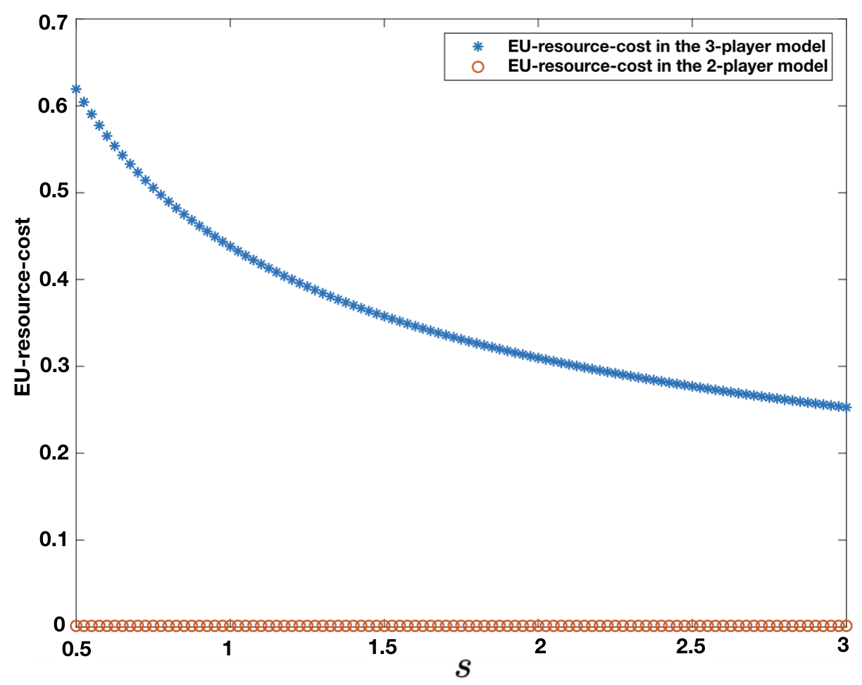 Figure 1
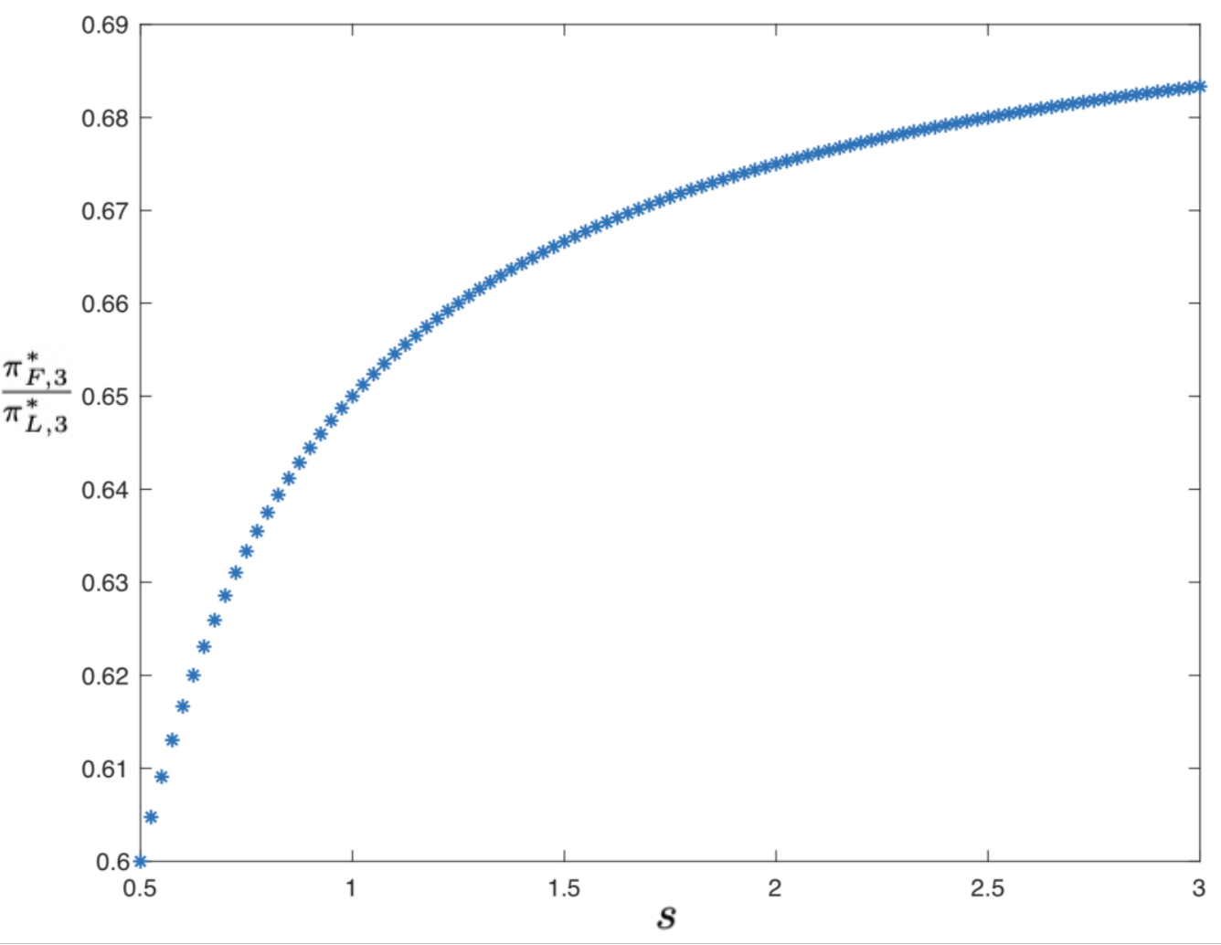 Figure 2
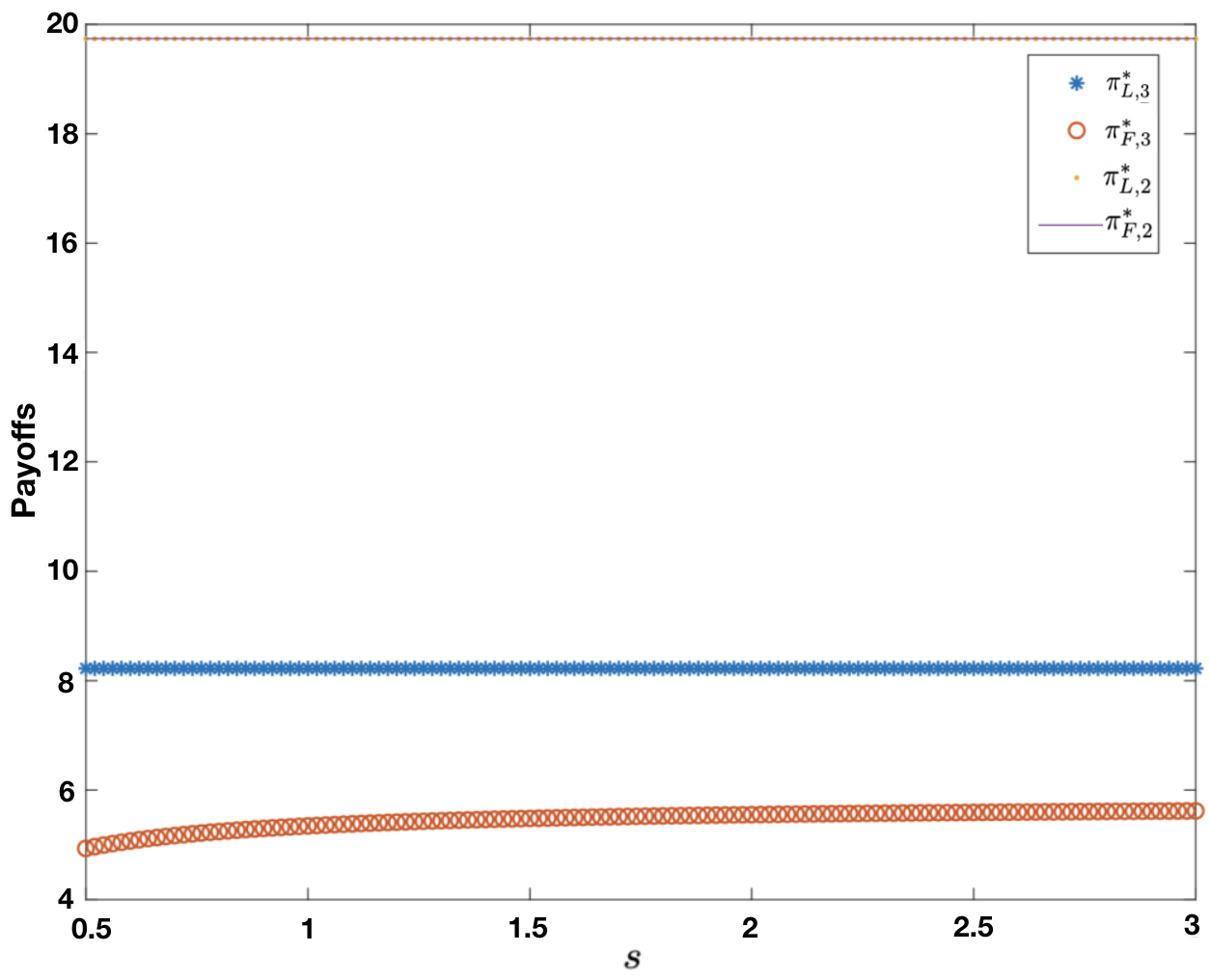 Figure 3
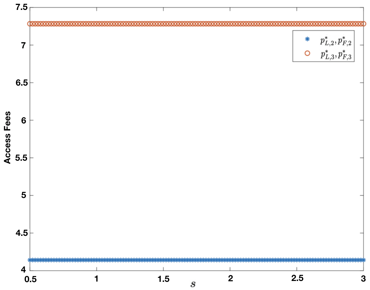 Figure 4
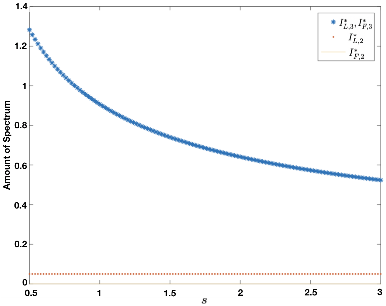 Figure 5
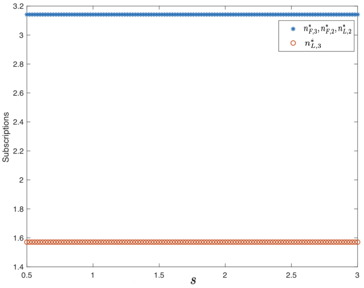 Figure 6
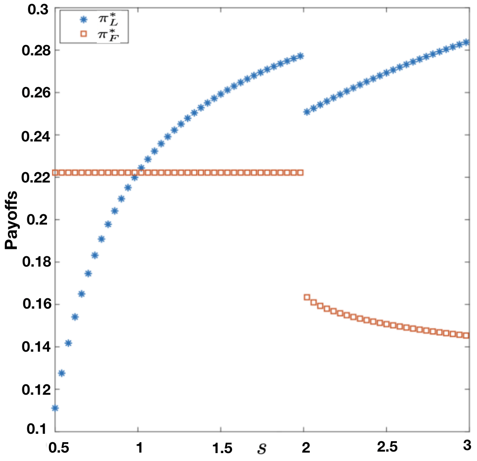 Figure 7
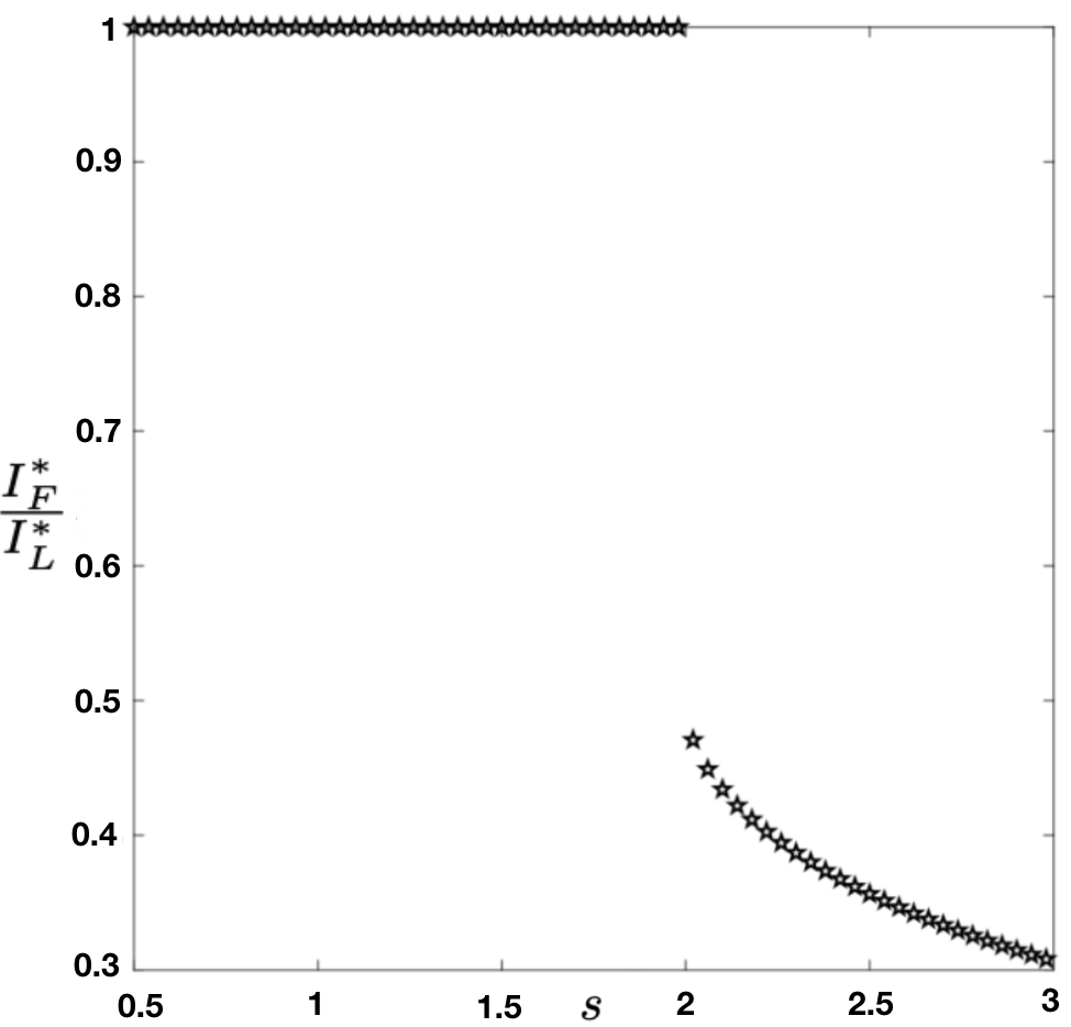 Figure 8
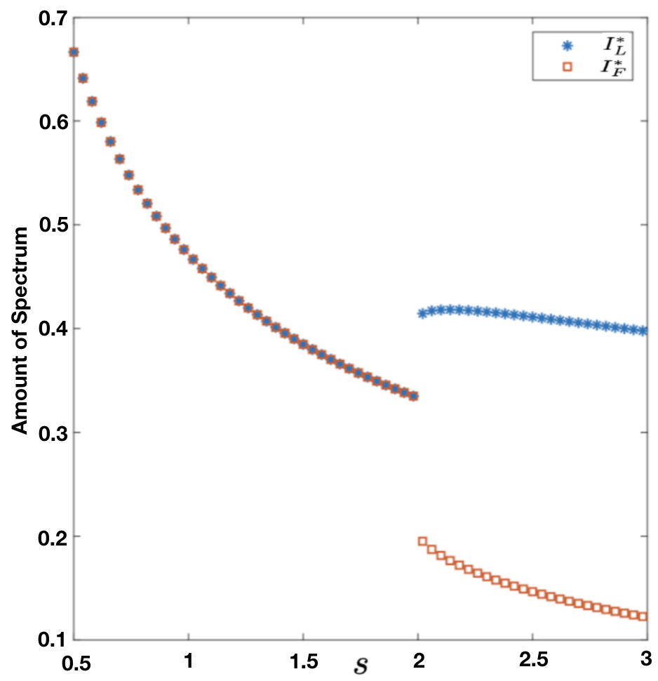 Figure 9
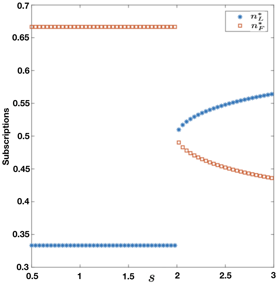 Figure 10
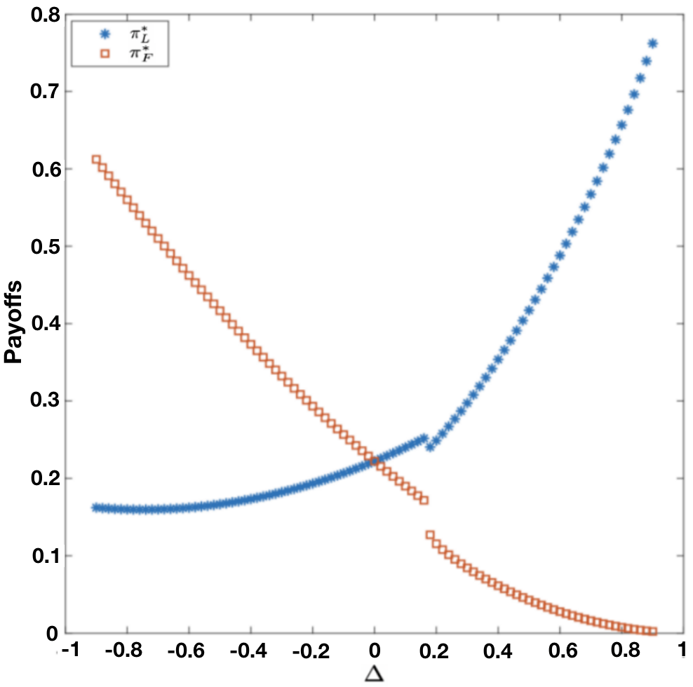 Figure 11
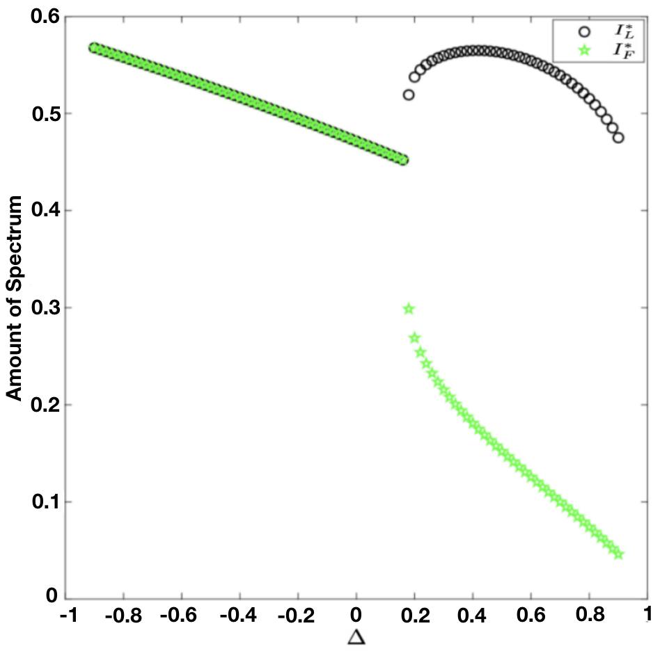 Figure 12
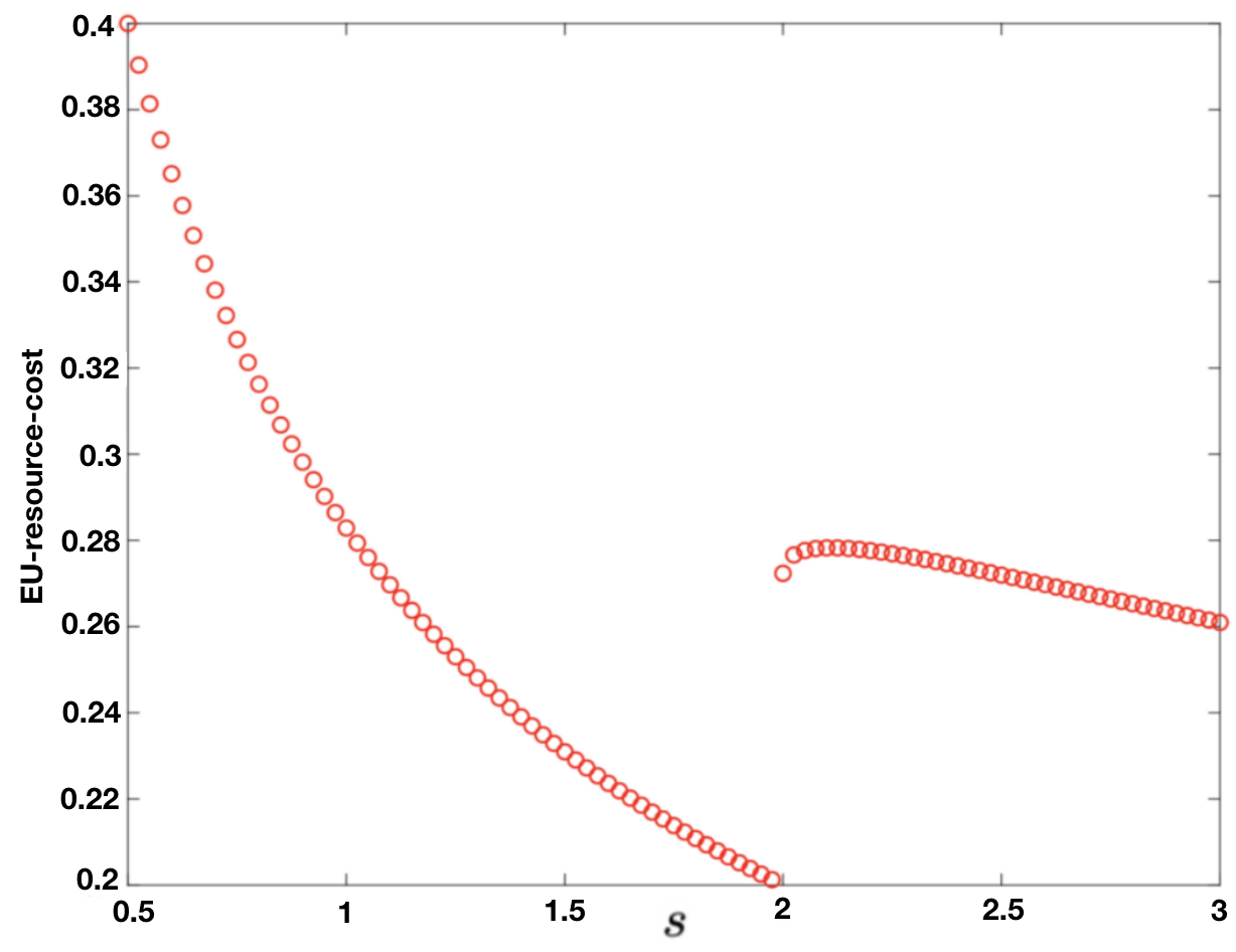 Figure 13
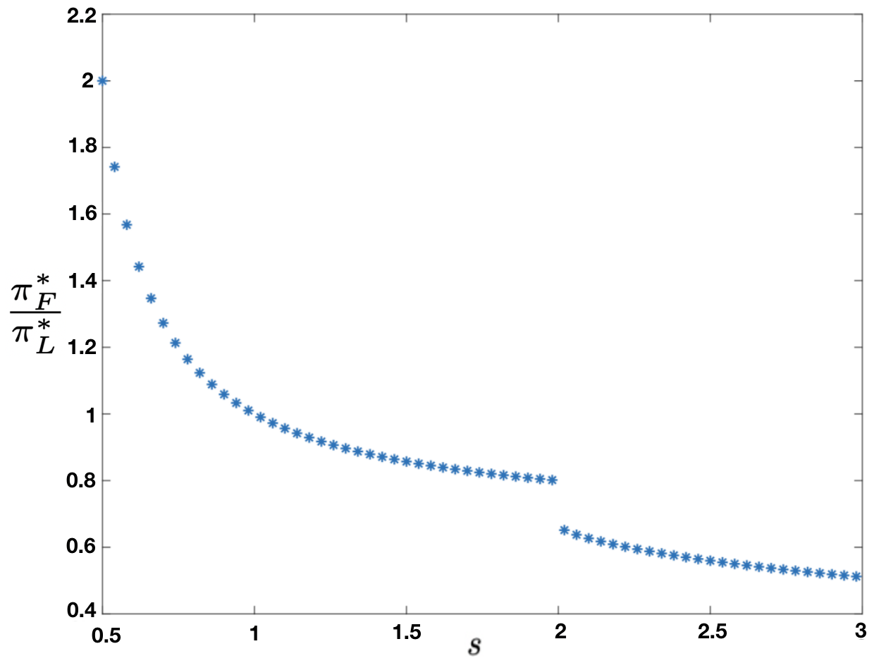 Figure 14
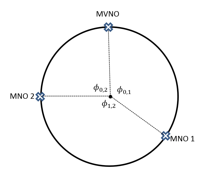 Figure 15
 Figure 16
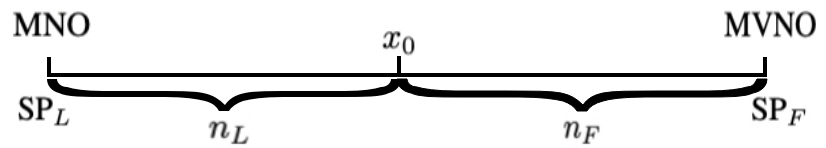 Figure 17
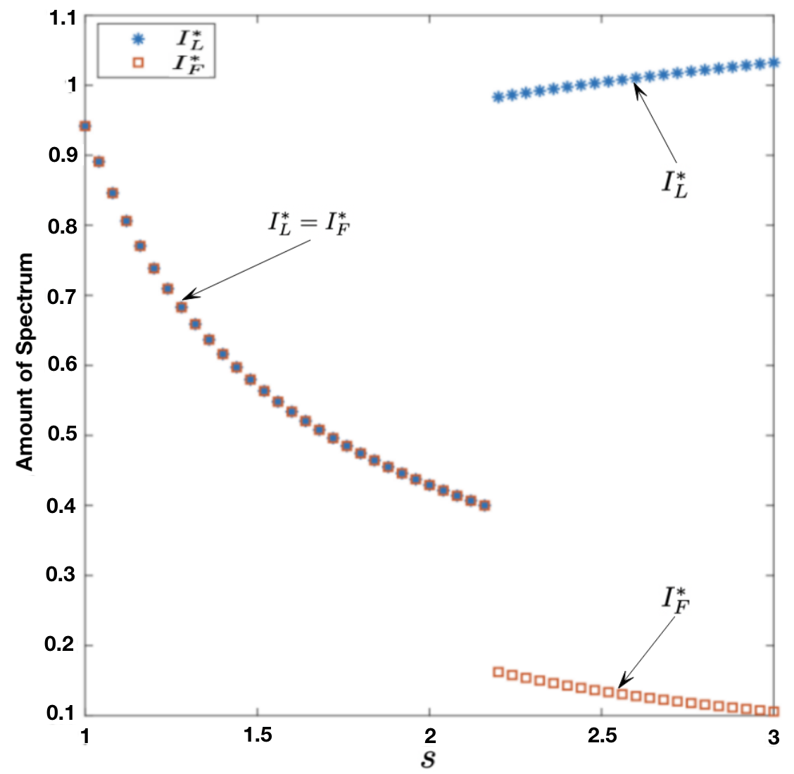 Figure 18
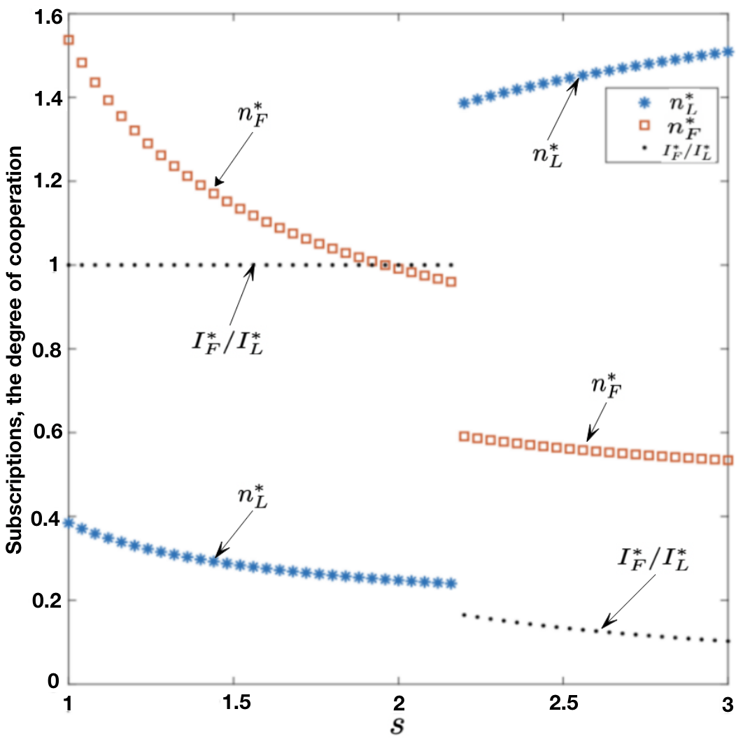 Figure 19
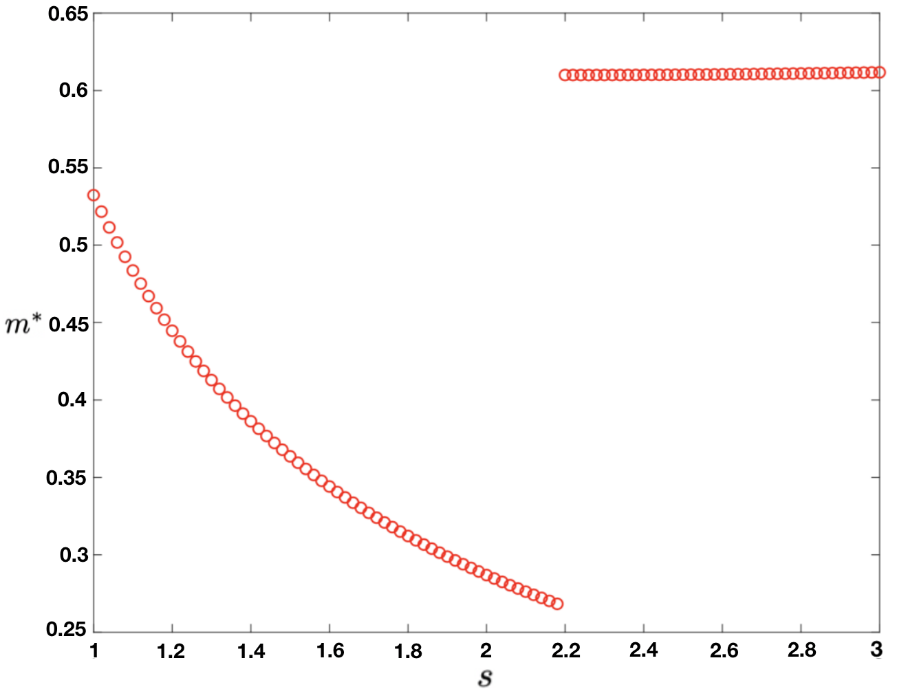 Figure 20
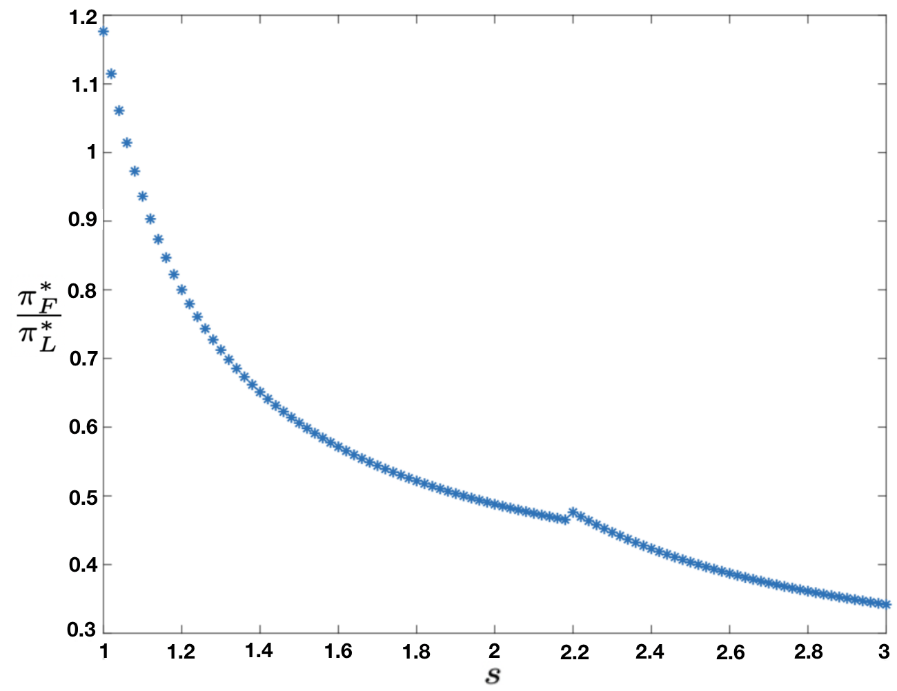 Figure 21
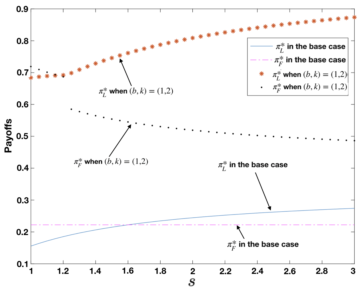 Figure 22
 Figure 23
 Figure 24
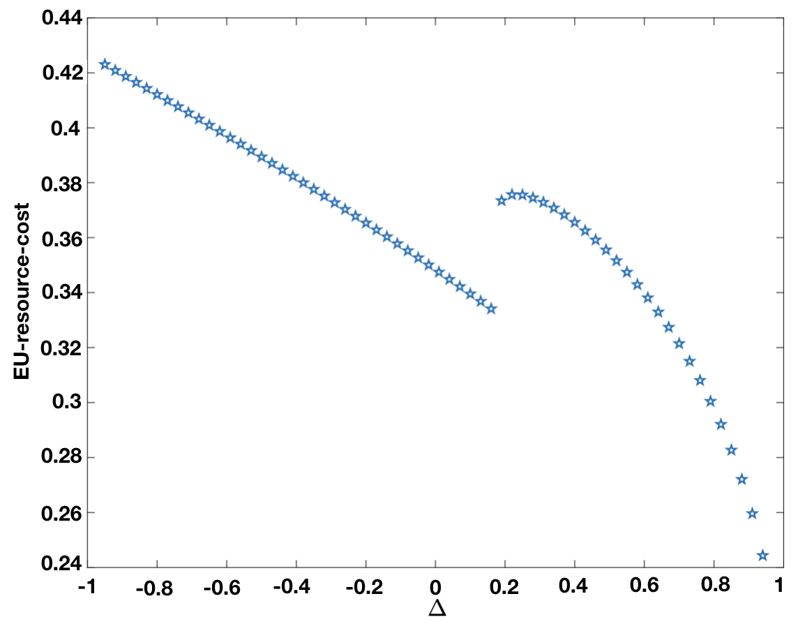 Figure 25
Peer Reviews
No public reviews on file for this paper yet. If you reviewed it on a platform where reviews are public (OpenReview, ICLR, NeurIPS, ICML), you can paste yours below so the community can read it here.
Videos
No videos yet. Explain this paper in a talk, walkthrough, or lecture? Add one.
Taxonomy
TopicsGame Theory and Applications · ICT Impact and Policies · Digital Platforms and Economics
Supplementary Material for the Paper “The Interplay of Competition and Cooperation among Service Providers (Part I)”
Xingran Chen, Mohammad Hassan Lotfi, Saswati Sarkar Xingran Chen and Saswati Sarkar are with the Electrical and System Engineering Department of the University of Pennsylvania, PA, 19104.
E-mail: [email protected], [email protected] Mohammad Hassan Lotfi is with the Institute for System Research of the University of Maryland, College Park, MD, 20740.
E-mail: [email protected] Parts of this work was presented in Annual Conference on Information Sciences and Systems (CISS), 2017.
Abstract
This paper investigates the incentives of mobile network operators (MNOs) for acquiring additional spectrum to offer mobile virtual network operators (MVNOs) and thereby inviting competition for a common pool of end users (EUs). We consider a base case and two generalizations: (i) one MNO and one MVNO, (ii) one MNO, one MVNO and an outside option, and (iii) two MNOs and one MVNO. In each of these cases, we model the interactions of the service providers (SPs) using a sequential game, identify when the Subgame Perfect Nash Equilibrium (SPNE) exists, when it is unique and characterize the SPNE when it exists. The characterizations are easy to compute, and are in closed form or involve optimizations in only one decision variable. We identify metrics to quantify the interplay between cooperation and competition, and evaluate those as also the SPNEs to show that cooperation between MNO and MVNO can enhance the payoffs of both, while increased competition due to the presence of additional MNOs is beneficial to EUs but reduces the payoffs of the SPs.
Index Terms:
Heterogeneous networks, Wireless Internet Market, Service Providers, Spectrum provisioning, Subscriber pricing, Game Theory, Hierarchical games, Nash Equilibrium
I Introduction
I-A Motivation and Overview
Nowadays wireless service providers (SPs) are divided into (i) mobile network operators (MNOs) that lease spectrum from a regulator like FCC, and (ii) mobile virtual network operators (MVNOs) that obtain spectrum from one or more MNOs. MVNOs can distinguish their plans from MNOs by bundling their service with other products, offering different pricing plans for End-Users (EUs), or building a good reputation through a better customer service. Although traditionally wireless service has been offered only by MNOs, in recent years, the number of MVNOs has been rapidly growing. The number of MVNOs increased by 70 percent worldwide, during June 2010-June 2015 reaching 1,017 as of June 2015 [6]. Even some MNOs developed their own MVNOs. An example of which is Cricket wireless which is owned by AT&T and offers a prepaid wireless service to EUs. Another example of MVNOs is the Google’s Project Fi in which the customer’s service is handled using Wi-Fi hotspots wherever/whenever they exist; elsewhere the service is handled using the spectrum of a number of MNOs, eg, Sprint, T-Mobile or U.S. Cellular networks.
In this work, we consider the economics of the interaction among MNOs and MVNOs. We seek to understand why and under what conditions the MNOs cooperate with the MVNOs by offering some of their spectrum to the MVNOs, and thereby inviting competition for a common pool of EUs. We consider scenarios where the MNOs decide on acquiring new spectrum, and in exchange for a fee offer those to MVNOs, which decide to acquire some of the spectrum offered. The SPs decide on their pricing strategies for the EUs, and the EUs decide to opt for one of them, or neither, if the access fees and the qualities of service are not satisfactory. The spectrum acquisition and pricing decisions of the SPs determine their respective profits. We characterize their equilibrium choices. We obtain metrics that quantify the cooperation and competition of the SPs in terms of their spectrum investments and subscriptions of EUs, which help quantify the interplay between competition and cooperation under the equilibrium choices.
We consider a hotelling model in which a continuum of undecided EUs decide which of the SPs they want to buy their wireless plan from, if at all. The EUs have different preferences for each SP. These preferences can be because of different services and qualities that SPs offer. For example, the MVNOs may be able to offer a free or cheap international call plan through VoIP, or an SP may have an infamous customer service. The preference for a SP also increases with the spectrum she acquires. If, for example, EUs have high preferences for MVNOs, then the MNOs may prefer to lease some of their spectrum to the MVNOs and receive their share of profit through the MVNOs, instead of competing for EUs by lowering their access fees. On the other hand, if EUs have high preferences for the MNOs, the MNOs may not offer spectrum to the MVNOs and seek to attract the EUs directly. Thus, cooperation is mutually beneficial only in some scenarios, which we seek to identify.
I-B Contribution
First, we consider a base case in which one MNO and one MVNO compete for EUs in a common pool, and the EUs must choose one of the SPs. We present the system model, important definitions and terminologies, and quantify metrics such as degree of cooperation and EU-resource-cost that we use to assess the system from the perspective of various stake-holders throughout (Section II-A). We consider a sequential game in which the SPs decide their spectrum investments and access fees for the EUs (Section II-B). We subsequently seek the Subgame Perfect Nash Equilibrium (SPNE) outcome of the game using backward induction, and identify conditions under which the SPNE exists and is unique, and characterize the SPNE whenever it exists (Sections II-C, II-E). The SPNE is simple to compute, as 1) the amount of spectrum the MNO invests turns out to be the value that maximizes a function involving only one decision variable 2) the amount of spectrum the MVNO leases from the MNO is a simple closed form expression involving the amount that the MNO offers it and the leasing fee 3) the access fees for the EUs constitute simple closed form expressions of the spectrum the SPs acquire. The characterizations provide several insights. The spectrum acquired by the MNO never falls below a threshold which depends only on the leasing fee to the MVNO and preferences for the SPs. When the spectrum equals this threshold, the MVNO reserves the entire spectrum that the MNO offers it. Thus cooperation is high in this case. As the MNO acquires higher amounts of spectrum, the MVNO reserves progressively lower amounts, leading to lower degrees of cooperation. Numerical computations reveal that the MNO acquires minimal amount of spectrum only when the leasing fee to the MVNO is smaller than a threshold (Section II-D). The SPNE characterizations show that higher degrees of cooperation invariably reduces (enhances, respectively) the efficacy of the MNO (MVNO, respectively) in competing for the EUs; yet, higher degrees of cooperation enhance the payoffs of both the SPs as our numerical computations reveal. The MNO’s loss in revenue from subscription is more than compensated by the leasing fees obtained from the MVNO.
Second, we generalize the hotelling model for EU subscription in the base case by incorporating an additional demand function (Section III). The effects of the demand function are two-fold. First, the demand function models the attrition in the number of EUs of SPs if the spectrum investment or price of both SPs is not desirable for EUs. Thus, in effect, an EU may opt for neither SP if neither offers a price-quality combo that is to his satisfaction, which is equivalent to opting for outside options. Second, the demand function models an exclusive additional customer base for each of the SPs to draw from depending on her investment and the price she offers. We characterize the unique interior SPNE outcome of the game (Section III-A). Numerical results reveal that the general behavior of the SPNE outcome are as in the base case and that the EU-resource-cost increases compared to the base case (Section III-B).
Finally, we generalize the base case to include competition between MNOs. We consider a wireless market with two MNOs and one MVNO, in which EUs choose one of the three SPs (Section IV). We generalize the hotelling model to consider three players instead of two in the classical ones (Section IV-A), and characterize the unique SPNE outcome (Section IV-B). The characterizations show that this enhanced competition 1) increases the degree of cooperation, as the MVNO acquires all the spectrum that the MNOs offer, and 2) is beneficial to EUs, as the amounts of spectrum of SPs acquires are higher, and the SPs charge the EUs less. Numerical results reveal that the additional competition enhances the EU-resource-cost compared to the base case.
I-C Relation with the Sequel
While in this work we consider that the SPs arrive at their decisions individually, in the accompanying sequel we consider that the SPs arrive at certain decisions as a group, and then arrive at other decisions individually (Part II). Also, here we assume that the per unit leasing fee the MVNO pays to MNO(s) is a fixed parameter, which is beyond the control of individual MNOs and MVNOs. This happens for example in two important cases: 1) when this fee is determined by an external regulator to influence the interaction between different providers (possibly to the betterment of the EUs) 2) when this fee is a market-driven parameter, for example, in a large spectrum market with many MNOs and MVNOs. To understand the impact of the externals (eg, regulator, market), we investigate the implications of different values of this fee on the SPNE and the payoffs and the EU-resource-cost metric. This would also guide the regulatory choice of this fee for the first case. Note that the overall market may consider several MNOs and MVNOs, whose presence we consider in the generalizations (Sections III, IV). In the sequel we consider that the SPs cooperatively characterize this fee as a decision variable in a bargaining framework (Part II).
I-D Positioning vis-a-vis the State-of-the-Art
Duan et. al made early contributions in the field of MVNOs [11], [12]. They formulated the interactions between one cognitive mobile virtual network operator (CMVNO) and multiple end-users as a multi-stage Stackelberg game, and showed that spectrum sensing could improve the profit of the CMVNO and payoffs of the users. Since they considered only one SP, the issue of competition or cooperation between multiple SPs did not arise. We investigate the interplay of cooperation and competition between different SPs, namely MNO and MVNO.
The economics of the interactions among multiple service providers have been extensively investigated. We focus on non-cooperative interactions in this paper as here we consider that the SPs arrive at their decisions individually. Non-cooperative games were considered for example in [10], [12], [14], and [15]. A general framework of strongly Pareto-inefficient Nash equilibria with noncooperative flow control was considered in [10]. Applying the framework to communication networks, it was shown that the Nash equilibria were not efficient. Intervention schemes, i.e., systems where users and an intervention device interact, were formulated in [13], and a solution concept of intervention equilibrium was proposed. The paper showed that intervention schemes could improve the suboptimal performance of non-cooperative equilibrium. [15] proposed wireless virtualization to investigate spectrum sharing in wireless networks.
However, these works did not consider both MNO and MVNO, whose roles are fundamentally different from each other. The MNO acquires spectrum from a central regulator, which it offers to MVNO in exchange of money, and the MVNO uses part of this spectrum. Both MNO and MVNO earn by selling wireless plans to the EUs; the MNO earns additionally by leasing spectrum to the MVNO. Thus, they make different decisions, which affect their subscriptions, and their payoffs have different expressions. Their decisions also follow different constraints: spectrum acquired by the MVNO is upper bounded by that acquired by the MNO, which constitutes the MNO’s decision variable, while the spectrum acquired by the MNO depend on the availability with the regulators, the availability does not constitute the decisions of any provider. The interaction between the MNO and MVNO lead to an interplay of competition and cooperation between them, which calls for innovations in the realm of modeling and analysis.
To our knowledge, the only papers in the genre of non-cooperative interactions that also consider interactions of the MNOs and MVNOs are [3], [4] and [5]. In [3] MNOs seek to maximize the joint profit of MNO and MVNO. The MNO’s selection of access fees is formulated as a maximization in which the sales of the MNO is expressed as a function of only the fee he selects. In contrast we consider that each SP seeks to maximize his individual profit and obtain the access fees they select and the spectrum they acquire, which also determine how the EUs choose between the SPs. Thus we need to dwell in the realm of a hierarchical game rather than a single stage optimization. A scenario very different from ours is considered in [4]: the SPs do not compete for consumer market shares but for the proportion of resource they are going to use. The interaction between the SPs is a hierarchical game in which the MNO and MVNO choose their access fees, the MVNO also decide investment in content/advertising. The access fees become roots of a fourth order polynomial equation which is computed numerically. The closest to our work is [5], which considers a dynamic three-level sequential game of spectrum sharing between one MNO and one MVNO. The focus is however complementary to ours. Unlike our work, [5] does not consider decisions of the 1) MNO pertaining to how much spectrum to acquire from a regulatory body 2) MVNO pertaining to how much of the MNO’s spectrum offer he ought to accept (he assumes that the MVNO uses the entire spectrum the MNO offers). We also generalize our model to consider multiple MNOs and an MVNO, which [5] does not. [5] however considers a decision of the MVNO that we do not, i.e., how much the MNO would invest in content generation. The EU subscription models are also entirely different. We consider a one-shot game involving a continuum of EUs in which the SP choice of each EU is based on his intrinsic preferences for the SPs and the spectrum investments of the SPs. [5] considers a multi-time slot game in which a discrete number of EUs choose between the SPs based on their experiences in the previous slots and their estimates of the quality of service the SPs they had not chosen apriori offer. The games we consider fundamentally differ in that the SPNE need not exist in ours (we identify necessary and sufficient conditions for its existence), while it always exists in that in [5]. By exploiting the structure of the game, we obtain closed form expressions for the various decisions we consider, in the SPNE, whenever it exists. [5] computes the SPNE only numerically through the solution of a multi-slot stochastic dynamic program (DP). Our SPNE characterization is easy to compute, while DPs usually suffer from the curse of dimensionality.
II Base case
We present the system model in which we formulate the payoffs and strategies of SPs, and the utilities and decisions of EUs (Section II-A). Next, we formulate the interaction between different entities as a sequential game (Section II-B). Subsequently, we characterize the conditions under for the existence and the uniqueness of the SPNE, obtain closed form expressions for the SPNE when it exists (Section II-C). We present numerical results in Section II-D. We prove the analytical results in Section II-E, Appendix B (Theorems 3, 4, 5, 6), and Appendix D-A (Theorems 1, 2).
II-A Model
We consider one MNO (, represents leader) and one MVNO (, represents follower) which compete for a common pool of undecided EUs. offers amount of spectrum (which it acquires from a regulator) to in exchange of money, and uses amount of this spectrum. Clearly, . For simplicity of analysis and formulation, we assume that , where is a lower bound of , which is a parameter of choice. This assumption is not significantly restrictive as may be chosen as low a positive quantity as one desires111All results extend, with some modifications, when we consider that is upper bounded by . Such bounds may apply when the central regulator has limited spectrum to offer. Refer to Section V for the deductions.. Both and earn by selling wireless plans to EUs; earns additionally by leasing her spectrum to . We assume that both SPL and SPF have access to separate spectrum, which they can use to serve the EUs who join them, above and beyond the amounts they strategically acquire. For example, a SPF like Google’s Project Fi serves customers using Wi-Fi hotspots and the spectrum of 3 MNOs (Sprint, T-Mobile or U.S. Cellular networks). Also, SPL may acquire additional spectrum from the regulator which it does not offer SP
We denote the marginal leasing fee (per spectrum unit) that pays the regulator as , marginal reservation fee pays to by , the fraction of EUs that and attract as and , respectively, and the access fee that and charge the EUs as and , respectively. Since wants to lease out some of her spectrum to with profit motive, it is reasonable to assume that . We assume that are pre-determined. The strategies of SPs are to choose the investment levels (, ) and the access fees for EUs (, ) so as to maximize their overall payoffs, which we formulate next.
SPF and SPL respectively earn revenues of from EU subscription, where is the transaction cost SPs incur in subscription. The transaction cost arises due to traffic management, billing and accounting services, customer service, etc. associated with each subscription. We have assumed such costs to be equal for all SPs, as they do not significantly vary across them. We expect the cost of reserving spectrum to be strictly convex, i.e. the cost of investment per spectrum unit increases with the amount of spectrum. Strictly convex costs do not satisfy the economy of scale; the regulator may mandate such structures to stop excessive acquisition by big SPs seeking to control the market, which has limited spectrum supply, and drive out smaller SPs or new entrants. Incidentally, several seminal works have considered strictly convex investment costs, e.g. [7] and [8]. For simplicity in analysis, we consider a specific kind of strictly convex cost function, namely quadratic, and discuss generalizations in Remark 3. That is, SPL incurs a spectrum acquisition cost of , and SPF pays to SPL a leasing fee of . Thus, the payoffs of SPs are:
[TABLE]
EUs: We use a hotelling model[1] to describe how EUs choose between the SPs. We assume that SPL is located at [math], SPF is located at , and EUs are distributed uniformly along the unit interval (Figure 1). The closer an EU to a SP, the more this EU prefers this SP to the other. Note that the notion of closeness and distance is used to model the preference of EUs, and may not be the same as physical distance. Let () be the unit transport cost of EUs for SPL (SPF), the EU located at incurs a cost of (respectively, ) when joining SPL (respectively, SPF).
[TABLE]
The EU at receives utilities respectively from SPL and SPF, and joins the SP that gives it the higher utility.
The first component of the utility functions comprises of the “static factors”, namely and of and , respectively. The static factor of a SP is the same for all EUs, which depends on the local presence, its existing spectrum beyond or and its reputation in the region, quality of the customer-service, ease of usage for the online portals, etc. However, the static factors do not depend on strategies of SPs, such as the access fees, the investment levels, etc.
The second component, i.e., or , is denoted as the “strategy factor”. The strategy factors depend on the strategies of the SPs, namely their access fees and the spectrum they acquire. Clearly, the utilities would decrease with the access fees, we consider the dependence to be linear. As SPF acquires greater fraction of the additional spectrum SPL offers him, SPF becomes more desirable and SPL less desirable to the EUs. Denote and . Then the impact of quality of service in the decision of EUs is captured through and . For example, when , i.e., SPF leases the entire spectrum from SPL and SPL can use none of it, then and . This gives SPF an advantage over SPL in attracting EUs. Similarly, even when , i.e., SPF leases no spectrum from SPL, and , SPL has an advantage over SPF. But subscription may still be divided in both the above extreme cases. This happens since both SPF and SPL have access to separate spectrum as reflected in the static factors . Note that the pair of transport cost () is one of the many functions that can be considered. We choose this model specifically since it captures the essence of the model, and is analytically tractable.
Finally, the strategy factors incorporate intrinsic preference of the EUs towards the SPs through the coordinate , which presents the local distance in the utility model. If an EU is for example close to SPF, is high and is low, and it is deemed to have a higher intrinsic preference for SPF, as compared to SPL. The intrinsic preference may be developed through pre-existing and ongoing relations the EU has with the SPs, e.g., if an EU is already availing of other services from a SP, the EU will have a stronger intrinsic preference for the SP, due to convenience of billing etc. Higher intrinsic preferences enhance utilities of the SP for the EUs. The impact of the strategies of the SPs on the EUs will depend on their intrinsic preferences for the EUs, which is captured in the term or in the utility. Note that the intrinsic preference is different for different EUs unlike the static factor.
We consider that and are sufficiently large so that the utility of EUs for buying a wireless plan is positive regardless of the choice of SP222 Note that all analytical results will depend on the difference of and , so absolute values of these (large or otherwise) do not have any impact on the SPNE choices of various entities.. Thus, each EU chooses exactly one SP to subscribe to, i.e., the market is “fully covered”. This is a common assumption for hotelling models. We would in effect relax this assumption in Section III.
SPF’s leasing of spectrum from SPL constitute an act of cooperation. Thus, we call the degree of cooperation. Since SPF and SPL compete to attract EUs, the split of subscription represent the level of competition. Since the amount of spectrum SPF leases from SPL determines the split of subscription, there is a natural interplay between cooperation and competition, that these metrics will enable us to quantify.
We develop the notion of EU-resource-cost to capture the spectral resource per unit access fee averaged over all EUs, which represents the “bang-for-the-buck” or “value for money” an average EU gets out of the system. For the EUs who choose the MVNO, the resource per head is . Thus, for these EUs the resource per head per unit fee is . Similarly, for the EUs who choose the MNO, the resource per head per unit fee is . Averaging over all the EUs, the resource per unit fee for an “average” EU then is, , which equals , since We therefore consider this as the expression for the EU-resource-cost. Clearly, higher values of the EU-resource-cost is beneficial for the EUs.
II-B The sequential game framework
The interaction among SPs and EUs can be formulated as a sequential game. As a leader of the game, makes the first move. The timing and the stages of the game are as following:
- •
Stage 1: decides on the amount of spectrum, , to acquire.
- •
**Stage 2: ** decides on the amount of spectrum to lease from , .
- •
Stage 3: and determine the access fees for the EUs, and , respectively.
- •
Stage 4: Each EU subscribes to the SP that gives it the higher utility.
Remark 1**.**
We assume that the decision of investments ( and ) happens before the decisions of access fees ( and ), guided by the fact that spectrum investment decisions are long-term ones, and are therefore expected to be constants over longer time horizons in comparison to subscription pricing decisions.
Definition 1**.**
[2, Chapter 6.2]** A strategy is a Subgame Perfect Nash Equilibrium (SPNE) if and only if it constitutes a Nash Equilibrium (NE) of every subgame of the game.
We refer to a SPNE choice of spectrum investments and access fees by the SPs as , and the EU subscriptions for the SPs under the same as , should a SPNE exist.
II-C The SPNE outcome
We next identify the conditions under which SPNE exists, characterize the SPNE when it exists, and examine its uniqueness.
We denote as . Since , in the expressions for utilities in (3), provides a near insurmountable disadvantage to one of the SPs through the static factors; this SP might have to choose a significantly lower price to recoup. Thus, we first focus on the range As stated before, we assume is small, and let , which reduces to in the special case that .
Theorem 1**.**
Let . The SPNE is:
(1)* any solution of the following maximization is ,*
[TABLE]
(2)* is characterized in*
[TABLE]
(3)* ,*
(4)* .*
Remark 2**.**
From (2), is unique once is given; from (3) and (4), is unique once and are given. Thus, every solution of the maximization in Theorem 1 (1) leads to a distinct SPNE. Thus, the SPNE is unique if and only if this maximization has a unique solution. Our extensive numerical computations suggest that this is the case.
The SPNE is easy to compute, despite the expressions being cumbersome. Otherwise, can be obtained as a maximizer of an expression that involves only one decision variable, , and fixed parameters . has been expressed as a closed form function involving and the fixed parameters have been expressed as closed form functions of and the fixed parameters
From Theorem 1 (3), the price the EUs receive from SPL (respectively, SPF) decrease (respectively, increase) with increase in the degree of cooperation (). Thus, since at least one of the SPs reduce the price, the EUs benefit from higher degree of cooperation.
From Theorem 1 (3) and (4), Thus, SPNE subscriptions of the SPs increase with increase in the access fees they announce. This counter-intuitive feature arises because the subscriptions also depend on the spectrum acquisitions of the SPs, through the transport costs and in the utilities specified in (3).
From Theorem 1 (1), in the SPNE, SPL acquires at least amount of spectrum. From Theorem 1 (2), when equals this minimum, then SPF reserves all the available spectrum, i.e., (note that is continuous at ). Thus, SPL can not use any of However, from Theorem 1 (4), SPL is still able to attract a positive fraction of EUs: since . This is because EUs have spectrum other than as captured in the values of .
From Theorem 1 (1) and (2), when exceeds its minimum value, then SPF reserves only a fraction of available spectrum (). Note that in this case, . Thus, the higher the amount of available spectrum, the lower would be the amount of spectrum reserved by SPF. Also, is decreasing with .
The SPNE depends on the static factors only through their difference . As expected, with increase (respectively, decrease) in , SPL (respectively, SPF) can increase his (respectively, her) access fee (respectively, ). The minimum value of his spectrum acquisition increases with decrease in , to offset the competitive advantage the static factors provide. Through our numerical computations, we elucidate how and the payoffs otherwise vary with .
The results illustrate the interplay between cooperation and competition. From Theorem 1 (4), the subscription (respectively, ) of SPL (respectively, SPF) decreases (respectively, increases) with the degree of cooperation (). Thus, the higher the degree of cooperation, lesser (respectively, greater) is the competition efficacy of SPL (respectively, SPF). A natural question arises: why would the SPL then cooperate with the SPF? From (1) and (2), Theorem 1 (3), (4), , and . On the one hand, if the degree of cooperation increases, then the amount of subscribers of SPL decreases, thus the revenue SPL earn from the subscribers decreases. On the other hand, the payoff of SPL increases through . Thus the second factor may offset the first, and the payoff of SPL may increase due to cooperation. Note that it is not a zero sum game, thus, the payoffs of both players may simultaneously increase due to cooperation. We illustrate these phenomena definitively through our numerical computations in the next section.
Then, in the extreme case that :
Theorem 2**.**
*(1) *** : The SPNE is
[TABLE]
*and can be chosen any value in
**(2) *** The following interior strategy constitute an additional SPNE:
[TABLE]
*(3) *** The SPNE strategy is:
[TABLE]
*and can be chosen any value in
We prove this theorem in Appendix D-B. As is intuitive, for large , all EUs subscribe to SPL, despite lower access fees selected by SPF; the reverse happens in the other extreme, despite lower access fees selected by SPF. The extremes therefore lead to “corner equilibria”, which correspond to as the degrees of cooperation. The SPNE is non-unique in both these extremes.
II-D Numerical results
Figure 2 shows the payoffs (left) and the degree of cooperation (right) under different when . The degree of cooperation reaches the maximum (), i.e., when is less than a threshold (). In this case, SPL generates most of its revenue from the reservation fee paid by SPF. As expected, increases with . From Theorem 1 (1), (2), (4), when , equals its minimum value , and , thus is a constant which is independent of . When is larger than this threshold, , and decreases with . In this case, exceeds its minimum value, and SPF leases only a portion of the new spectrum invested by SPL, i.e., . Thus, SPL generates more of its revenue from EUs. The payoff of SPL (SPF) first jumps to a lower value at this threshold, and then increases (decreases) with . At this threshold, the degree of cooperation also jumps to a lower value (). Thus, higher degrees of cooperation can enhance the payoff of both SPs, and the reservation fee enhances (reduces) the payoff of SPL (SPF). Also, SPF earns more than SPL for lower values of ; hence SPF gets more from the spectrum sharing between the 2 SPs in this case. For higher values of , the reverse happens.
has significant impact on the EU-resource-cost, as depicted in Figure 3. We first explain the jump at the threshold value of . When is less than the threshold, , as seen in Figure 2 (right). Thus the EU-resource-cost is . At the threshold, , so the second term in EU-resource-cost () jumps to a positive value from [math], leading to the jump in the EU-resource-cost. The EU-resource-cost otherwise decreases in , thus if a regulator chooses , it ought to opt for a low value of , though if is really low, then SPL may not have enough incentive to cooperate due to low (Figure 2 (left)). Note that the degree of cooperation is at low values of , thus high degree of cooperation coincides with high EU-resource-cost.
Figure 4 shows the SPNE level of investment (left) and subscriptions of SPs (right) when . It reconfirms that when is smaller than a threshold, SPF leases the entire spectrum SPL offers, and after that threshold, SPF leases only a portion of the new spectrum offered by SPL. Also, strictly decreases with throughout. When is small, , and are constant (, ) independent of and , and . After the threshold, decreases and increases with (because decreases with in Figure 2 (right)). Comparing Figure 2 (right) and Figure 4 (right) we note that higher degrees of cooperations increase (decrease, respectively) the competition efficacy of SPF (SPL, respectively).
Figure 5 plots the payoffs (left) and , (right) as a function of when , the region in which the SPNE exists uniquely. We set . As expected, the payoff of SPL (SPF, respectively) increase (decrease, respectively) with increase in . Also, SPF earns more than SPL for lower values of ; hence SPF gets more from the spectrum sharing between the 2 SPs in this case. For higher values of , the reverse happens. With increase in , , may either increase or decrease, depending on whether additional spectrum provides “bang for the buck” by enticing commensurate number of EUs which depends on the EUs’ prior biases (static factors) for or against the SPs. The figure shows which is the case.
Figure 6 plots the degree of cooperation (left) and the EU-resource-cost (right) as a function of when . Figure 6 (left) shows that the degree of cooperation is a constant when is less than a threshold, and decreases when is larger than this threshold. The amount of spectrum SPF leases from SPL decreases when SPL has larger common preference. The jump in the EU-resource-cost at the threshold value of may be explained similar to that for Figure 3, considering Figure 6 (left) instead of Figure 2 (right). Other than this jump, the EU-resource-cost decreases in Again, note that high degree of cooperation coincides with high EU-resource-cost.
II-E SPNE Analysis
We use backward induction to characterize SPNE strategies, starting from the last stage of the game and proceeding backward. For simplicity and brevity, we present this analysis only for the important special case of , and defer the general case to Appendix B. Thus, we prove Theorem 1 while applying in the corresponding expressions. Specific Theorems 3, 5, 6 are proven in Appendix B.
Stage 4: We first characterize the equilibrium division of EUs between SPs, i.e., and , using the knowledge of the strategies chosen by the SPs in Stages 13.
Definition 2**.**
* is the indifferent location between the two service providers if (Figure 1).*
By the full market coverage assumption, if , then EUs in the interval join and those in the interval join . If , all EUs choose ; and if , all EUs choose (Figure 1).
From Definition 2, . Since , then . Thus,
[TABLE]
Thus, since EUs are distributed uniformly along , the fraction of EUs with each SP is:
[TABLE]
where is defined in (4) and (Figure 1).
Only “interior” strategies may be SPNE, as:
Theorem 3**.**
In the SPNE it must be that
Stage 3: SPL and SPF determine their access fees for EUs, and , respectively, to maximize their payoffs.
Lemma 1**.**
The payoffs of SPs are:
[TABLE]
Proof.
From (5), substitute into (1) and (2), and get (6). ∎
We next obtain the SPNE and which maximize the payoffs and of the SPs respectively.
Theorem 4**.**
The SPNE pricing strategies are:
[TABLE]
Proof.
and must satisfy the first order condition, i.e., and . Thus, . and are the unique SPNE strategies if they yield and no unilateral deviation is profitable for SPs. We establish these respectively in Parts A and B.
Part A. From (7), . Since and , then .
Part B. Since , a local maxima is also a global maximum, and any solution to the first order conditions maximize the payoffs when , and no unilateral deviation by which would be profitable for the SPs. Now, we show that unilateral deviations of the SPs leading to and is not profitable. Note that the payoffs of the SPs, (1) and (2), are continuous as , and (which subsequently yields and , respectively). Thus, the payoffs of both SPs when selecting and as the solutions of the first order conditions are greater than or equal to the payoffs when and . Thus, the unilateral deviations under consideration are not profitable for the SPs. ∎
Remark 3**.**
The proof shows that do not depend on the specific nature of the costs of leasing spectrum , neither does from (5). Thus the SPNE expressions for these would remain the same for any other cost function. But, the SPNE of investment levels (, ) as obtained in the next results depend on the specific nature of these functions.
Stage 2: SPF decides on the amount of spectrum to be leased from SPL, , with the condition that , to maximize .
Theorem 5**.**
The SPNE spectrum acquired by is:
[TABLE]
Stage 1: SPL chooses the amount of spectrum to lease from the regulator, to maximize .
Theorem 6**.**
The SPNE spectrum acquired by SPL, is the solution of the following maximization
[TABLE]
Let . Theorem 1 follows from Theorems 3, 4, 5, 6. Theorem 3 allows us to consider only interior SPNE. Parts (1) and (2) of Theorem 1 follow respectively from Theorems 6 and 5. Part (3) follows from Theorem 4, part (4) from Theorem 4 and (5).
III EUs with Outside Options
We now generalize our framework to consider a scenario in which the EUs from the common pool the SPs are competing over, may not choose either of the two SPs if the service quality-price tradeoff they offer is not satisfactory. In effect, there is an outside option for the EUs. Also, each SP has an exclusive additional customer base which can provide customers beyond the common pool depending on the service quality and access fees they offer. We introduce these modifications through demand functions we describe next.
Definition 3**.**
The fraction333The fraction may be replaced with actual number (of EUs) in this case, by altering scale factors in this expression and in those of the payoffs. Our results hold for both interpretations as we do not use in any derivation. We use though. of EUs with each SP is
[TABLE]
where
[TABLE]
and , , and are constants.
Here, represent fractional subscriptions from the common pool as before, and are determined in Stage 4 of the sequential game described in Section II-B, based on the utilities specified in (3), with for simplicity. The demand functions and can be positive or negative. A positive value denotes attracting EUs presumably from an exclusive additional customer base beyond the common pool, and a negative value denotes losing some of the EUs in the common pool to an outside option. The size of the common pool may be different from the exclusive additional customer bases of the SPs; to account for this disparity, we multiply the fractional subscriptions from the common pool, with a constant
Considering , for analytical tractability:
[TABLE]
with , , and
[TABLE]
The formulation is the same as in Sections II-A, II-B, with replacing in (1) and (2). Using the argument that led us to the expression for the As in Section II-A, the EU-resource-cost is , following the argument in the last paragraph of Section II-A. We characterize the SPNE strategies in Section III-A, and provide numerical results in Section III-B.
III-A The SPNE outcome
For simplicity, we consider only interior SPNE strategies, that is, . We define functions , , and sets , as follows:
[TABLE]
[TABLE]
[TABLE]
With , we prove in Appendix E:
Theorem 7**.**
The interior SPNE strategies are:
- (1)
* is characterized in*
[TABLE]
- (2)
* is characterized in*
[TABLE]
- (3)
, .
- (4)
,
Remark 2 holds here with Theorem 7 substituting Theorem 1.
Despite the expressions being cumbersome, the characterization is easy to compute, as in Theorem 1, and lead to important insights, as enumerated below.
[TABLE]
In both equations, intuitively, the first term, , represents the subscription from the common pool, if there had been no attrition to an outside option. The second and third terms represent the impacts of the attritions as also the additions from the exclusive customer bases. The first term depends on the degree of cooperation similar to the the base case specified in part (4) of Theorem 1. In the special case that , i.e., when the demand functions depend only on the access fees, the third term is [math] and the demand functions capture the impact of attrition and additions in the SPNE expression for the subscriptions. For , the second and the third term together become in the expression for , and in that for . Thus, higher degree of cooperation decreases (increases, respectively) the subscription for SPL (SPF, respectively) even in these terms, and therefore, overall, like in the base case. Note that the subscriptions represent the efficacy in competition. However, as in the base case, the decrease in subscription does not directly lead to reduction in overall payoffs of SPL, as the deficit may be compensated through income generated by leasing spectrum to SP
III-B Numerical results
Figure 7 show that now, both can decrease (eg, with changes in ) because of attrition to the outside option possibly due to decrease of We note this when is below a threshold. Otherwise, the trends resemble Figures 2 and 4 (the base case).
Figure 8 (left) shows the payoffs under different . The trends of payoffs are similar with Figure 2 (left). The SPs earn higher payoffs than in the base case, as they have additional exclusive customers bases to draw additional EUs from.
Figure 8 (right) shows that for different values of the parameters , the EU-resource-cost exceeds that for the base case shown in Figure 3. This is because the SPs provide better resource-cost tradeoff to the EUs so as not to loose them to the outside option, and also to draw more EUs from their exclusive additional bases.
IV The 3-player model
We now generalize our framework to consider competition between MNOs, rather than that only between an MNO and an MVNO. In a 3-player model, we consider two MNOs and one MVNO competing for a common pool of EUs in a covered market (i.e., each EU needs to opt for exactly one SP). We present the model in Section IV-A, and characterize the SPNE in Section IV-B. We show that the competition among multiple SPs reduces their payoffs, but benefits the EUs: the SPs acquire higher amounts of spectrum (hence provide higher service quality), and charge the EUs less. The competition also reduces the payoffs of SPs. We prove the results in Appendix C (Theorems 8, 9) and in Section F (Corollary 1).
IV-A Model
We consider a symmetric model and seek a symmetric equilibrium i.e., the strategies of the MNOs are the same, and the MVNO leases the same amount of spectrum from each MNO. Thus, in the SPNE, , , , and . The total amount spectrum of SPs is . Thus, each MNO retains spectrum. We define the payoffs of MVNO and MNOs as
[TABLE]
To accommodate the three SPs, we modify the hotelling model. The EUs are uniformly distributed along a circle of radius 1 on which the SPs are virtually located (Figure 9). Since the radius is , each arc length equals the corresponding angle. Thus, the number of EUs located 1) between the MVNO and MNOi is and 2) between the MNOs is .
We consider that , and reflect the natural preferences of EUs for SPs (intuitively, for example, those in the arc would have stronger preference for the MVNO and MNO1, and so on). We allow the preferences to depend on spectrum investments by defining these arcs as: and for some functions and (considering that the model is symmetric). We can now consider the transport cost as a parameter rather than a function of , unlike in Section II. We focus on the special case that .
Similar to (3), if an EU is located in the arc of , at a distance of from the MVNO,
[TABLE]
By calculation, if , then , and . Then, EUs choose MVNO. If , then , and . Then, EUs choose MNO1 instead of MNO2.
Similarly, due to symmetry, if an EU is located in the arc of , he does not choose MNO1, and suppose the distance from the EU to the MVNO is , thus
[TABLE]
If an EU is located in the arc of , at a distance of to the MNO1, then his utility is;
[TABLE]
Now we have the following lemma,
Lemma 2**.**
If , then all EUs choose the MVNO; if , then EUs located in the arc of do not choose the MVNO.
Henceforth, we only consider , as:
Theorem 8**.**
No SPNE strategy exists if .
Now, from Lemma 2 and the discussion above, the MVNO and MNOi (MNO1 and MNO2, respectively) compete to attract the EUs located only on the arc of (, respectively). Thus, we define the number of EUs of any two SPs depends only on their total investment levels, i.e., for a constant ,
[TABLE]
IV-B The SPNE outcome
With , we prove in Appendix C:
Theorem 9**.**
The unique symmetric SPNE strategy, with representing the choices of, and subscription to, each MNO, and the corresponding quantities for the MVNO, is:
[TABLE]
Remark 4**.**
The MVNO leases the entire new spectrum from each MNO. The degree of cooperation, is The characterization of the SPNE is easy to compute.
We compare the outcome of the 3-player model with the 2-player model, to understand the impact of the competition between the MNOs. To ensure consistency of comparison, we modify the 2-player model of the base case in Section II as follows: (1) The transport cost is instead of and . (2) EUs are distributed uniformly along the interval instead of , since in the 3-player model, the total amount of EUs is (3) . By the same analysis method in Section II, we prove in Appendix F:
Corollary 1**.**
In the 2-player game formulation, the unique SPNE strategies are:
[TABLE]
Comparing Theorem 9 and Corollary 1, we note that due to the competition by an additional MNO, SPs acquire higher amounts of spectrum in the 3-player model, i.e., the two MNOs order additional spectrum, and the MVNO leases the entire new spectrum from each MNO. The SPs charge the EUs less too: , as opposed to in the 2-player model. In both models, the MNO(s) and the MVNO divide the EUs equally: in the 2-player model, each SP has half of the EUs (), while in the 3-player model, the MVNO has half of the EUs (), and each MNO has a quarter of the EUs ().
From (12) and (13), for 3 players, the payoffs are: (1) for each MNO, and (2) for the MVNO. For 2 players, the payoffs are and for the MNO and the MVNO respectively. Thus, clearly (each) MNO secures a higher payoff than the MVNO for both the -player and the player cases. Also, the SPs earn more in the 2-player model, since fewer SPs compete for the same number of EUs.
Since there are MNOs and MVNO now, and the MVNO leases amount of spectrum from each MNO, the EU-resource-cost becomes
IV-C Numerical results
In Figure 10 (left), (respectively, ) are investment levels of SPs in 3-player (respectively, 2-player) model, comparing Theorem 9 and Corollary 1, we note that due to the competition by an additional MNO, SPs acquire higher amounts of spectrum in the 3-player model, i.e., the two MNOs order additional spectrum, and the MVNO leases the entire new spectrum from each MNO. From Figure 10 (right), (respectively, ) are access fees of SPs in 3-player (respectively, 2-player) model, the SPs charge the EUs less too: , as opposed to in the 2-player model.
Figure 11 (left) shows that SPs can gain less if an additional MNO enters the system due to the additional competition. Figure 11 (right) shows that the EU-resource-cost in the -player model exceeds that in the base case for 2 SPs shown in Figure 3. This follows because as noted earlier EUs pay lower access fees and the SPs acquire higher spectrum overall. Thus, like in Section III-B, the additional competition among the SPs is beneficial for the EUs.
V Generalization: Limited Spectrum from the Central Regulator
Since we have assumed the spectrum available to the central regulator is limited. A natural assumption is that to set an upper bound to the investment level of SPL, . In this section, we assume . Similar with the assumption of , is parameter of choice. After considering the new condition of , we characterize the SPNE of the three cases above as follows. The proofs of Theorems 10, are given in Appendix G.
V-A The Base Case
Theorem 10**.**
Let . The SPNE is:
(1)
If , , .
(2)
If , the SPNE are the same as that in Theorem 1.
Theorem 11**.**
**(1) *** : The SPNE is the same as that in Theorem 2 (1).
**(2) *** The following interior strategy constitute an additional SPNE, if ,
[TABLE]
If , the SPNE is the same as that in Theorem 2 (2).
*(3) *** The SPNE strategy is: If , then
[TABLE]
If , the SPNE is the same as that in Theorem 2 (3).
From Theorems 10 and 11, we can find that if the upper bound is relative small, the MNO acquires the maximum amount of spectrum from the regulator, and the MVNO leases all spectrum from the MNO.
V-B EUs with Outside Options
For simplicity, we consider only interior SPNE strategies, that is, . We define sets , as follows:
[TABLE]
[TABLE]
With , we have the following SPNE:
Theorem 12**.**
The interior SPNE strategies are:
- (1)
* is characterized in*
[TABLE]
- (2)
* is characterized in*
[TABLE]
- (3)
, .
- (4)
,
The proof of Theorem 12 is the same as the proof of Theorem 7. Comparing Theorems 12 and 7, after adding the new condition on , the only change is that the region of is shrinked by the upper bound.
V-C The 3-player model
With , we have:
Theorem 13**.**
The unique symmetric SPNE strategy, with representing the choices of, and subscription to, each MNO, and the corresponding quantities for the MVNO, is:
(1)
If , then
[TABLE]
(2)
If , the SPNE is the same as that in Theorem 9.
Similar with Theorem 10, if the upper bound is relative small, the MNO acquires the maximum amount of spectrum from the regulator, and the MVNO leases all spectrum from the MNO.
VI Conclusions and Future Research Directions
This paper investigates the incentives of mobile network operators (MNOs) for acquiring additional spectrum to offer mobile virtual network operators (MVNOs) and thereby inviting competition for a common pool of end users (EUs). We consider a base case and two generalizations: (i) one MNO and one MVNO, (ii) one MNO, one MVNO and an outside option, and (iii) two MNOs and one MVNO. We identify metrics ( for cooperation between SPs, for competition between SPs, for resource-cost tradeoff of the EUs) to quantify the interplay between cooperation and competition. Four-stage noncooperative sequential games are formulated and SPNE are obtained analytically.
Analytical and numerical results show that higher degree of cooperation can enhance the payoff of both SPs, and increase (respectively, decrease) the competition efficacy of SPF (respectively, SPL). In addition, high degree of cooperation coincides with high EU-resource-cost, and provides low access fee options to the EUs. Increased competition due to the presence of additional MNOs is beneficial to EUs but reduces the payoffs of the SPs.
All results extend, with some modifications, when we consider that is upper bounded by . Such bounds may apply when the central regulator has limited spectrum to offer. In this case, if the upper bound is relatively small (less than some threshold), in the SPNE, , but otherwise characterized in various Theorems apply. The thresholds will in general be different for different cases and have been quantified. The SPNE values of the other decisions variables, namely remain as in various Theorems. Refer to Section V of the technical report [9] for the deductions.
Future research includes generalization to accommodate: 1) non-uniform distribution of EUs between the two SPs in the hotelling model, 2) distinct transaction costs and , 3) potentially non-convex spectrum reservation fee functions that the SPF pays the SPL and the SPL pays the regulator, 4) arbitrary number of MNOs and MVNOs, 5) arbitrary transport cost functions of the spectrum acquired by the SPs, . We next provide research directions in each.
If the EUs are non-uniformly distributed in , one can start with a cumulative distribution function which gives the fraction of EUs in . Starting with the base case and , in (5), for , will now be , where is given by (4), as before. Following the analytical progression in Section II-E, the results must now be derived using specific expressions for (eg, Lemma 1, Theorems 4, 5, 6). This will in turn help determine how the characteristics of the distribution function affect the equilibrium closed forms, which currently remains open. 2. 2.
The EUs may incur different amounts of transaction costs for the SPs, namely respectively for SPF, SP Starting with the base case, (4), (5) continue to hold. But, need to be replaced by respectively in the expressions for the payoffs in Lemma 1. Also, need to be replaced by respectively in the expressions for the access fees in Theorem 4. The expressions in Theorems 5, 6 must now be derived and modified, building on the above modifications. This derivation remains open. 3. 3.
Following Remark 3, the SPNE of investment levels (, ) remain open for an arbitrary spectrum reservation fee function that the SPF pays the SPL and the SPL pays the regulator. The analytical methodology used in Theorems 5, 6 should however apply, though the expressions would depend on the specific function in question. 4. 4.
To obtain the SPNE for arbitrary number of MNOs and MVNOs, one may distribute them on a circle as for 3 SPs (refer to Section IV-A and Figure 9), and follow the analytical approach presented in Sections IV-A, IV-B. The limitation of this distribution of SPs on a circle is that a SP can compete for EUs with only other SPs, as a SP can have only adjacent SPs and effectively only a pair of SPs compete for the EUs in the segment of the circumference between them. For SPs, this is not restrictive, as each SP anyway has no more than SPs to compete with, but it is restrictive for SPs when as there in general each SP competes with other SPs. Nonetheless, our circular distribution method provides a foundation for this general problem, by allowing SPNE computation for arbitrary number of SPs when each SP competes for EUs with predetermined SPs. More innovative topology of placements of SPs involving distributions in potentially higher dimensions may be able to relax this restriction, which remains open. 5. 5.
For arbitrary transport cost functions, the analytical methodologies (eg, Section II-E for the base case) would apply. But the derivation of the results remain open.
Appendix A On quadratic function maximization
Lemma 3**.**
Define a quadratic function with . The maximum of in an interval can be obtained by the following rules:
- (1)
If , and define the midpoint of the interval , then if ; if .
- (2)
If , i.e., is concave, then if ; if ; if .
Proof.
(1). Since , then is convex, thus the maximum point can only be obtained at the boundary points, i.e., or . Thus,
[TABLE]
Let . Since , . Note , from (17), , which implies . Similarly, if , note , then . Since , then from (17), , which implies .
(2). If , then is concave. Since , then 1) and is decreasing if , 2) and is increasing if . (i) If , then is decreasing if , hence . (ii) If , then is increasing if , hence . (iii) Let . Since is concave, thus has a unique maximum point (stationary point) , i.e., for all . If contains , i.e., , then for all , hence . ∎
Appendix B Proofs in the Base case when
Proof of Theorem 3 when .
Proof.
Let be a corner SPNE strategy. Thus, 1) , or 2) . We arrive at a contradiction for 1) Step 1 and 2) in Step 2 respectively.
Lemma 4**.**
. If
Proof.
Let . Consider a unilateral deviation in which From (12), , leading to a contradiction. Now, let and . Thus, which is a contradiction. ∎
Step 1. Let . Clearly, and . From (2),
From Lemma 4, Thus, From (4), . Thus, .
From (1), If , then since . Consider a unilateral deviation by which , then , which is beneficial for SPL. Thus, .
Now, let Thus, . Recall that Consider a unilateral deviation by which . Now, by (4), , and hence Now, from (2), . Thus, is not SPF’s best response to SPL’s choices , which is a contradiction. Hence,
Now consider another unilateral deviation of SPL, , where , with all the rest the same. Since ,
[TABLE]
Then
[TABLE]
The last inequality follows because and Thus, we again arrive at a contradiction.
Step 2. Let Clearly, . Since , by Lemma 4, . From (4), . Thus, Now, from (1),
[TABLE]
Consider a unilateral deviation by SPL, by which , . Then
[TABLE]
Therefore, by (62),
[TABLE]
Since , either or . If , then let . Then, . If , then (otherwise , which by Lemma 4 implies that is not a NE), then . Thus, . We again arrive at a contradiction. ∎
By Theorem 3 proved above henceforth we only consider interior SPNE in which
Proof of Theorem 5 when .
Proof.
Substituting and from (7) into (6), using and , ’s payoff becomes,
[TABLE]
Thus, the following maximization yields :
[TABLE]
(A). If , i.e., , is increasing in Thus, .
(B). Let . Referring to the terminology of Lemma 3, , which we denote as .
(B-1). Let , i.e., . Then is a convex function. Note that , and the midpoint of the interval is . From Lemma 3, since , then , the maximum is obtained at .
(B-2). Let , i.e., . Then is a concave function. Note that . From Lemma 3, and , thus
[TABLE]
Combining (A) and (B), we obtain (8). ∎
Proof of Theorem 6.
Proof.
Substituting and from (7) into from (6), using and , ’s payoff becomes:
[TABLE]
Now, the following optimization yields :
[TABLE]
Then, we have the following two sub-cases.
(A). From (8), if , then , thus for in this range, the objective function of the optimization is This is an increasing function of , since Thus the optimum solution for is .
(B). Next, if , then . Since when , then is continuous at . So as . Therefore, this case also includes the optimum solution of previous case. Thus substituting to (66), (9) is obtained. ∎
Appendix C The proofs in the 3-player model
Proof of Lemma 2.
Proof.
First, let . Consider EUs in the arc of . Consider an EU at distance from MNO1. From the symmetry of MNO1 and MNO2, 1) if , , and 2) if , Since , 1) if , then , and 2) if , then . Thus, all the EUs in arc will choose the MVNO.
Note that . Now consider the EUs in arc (), at a distance of from MNO1 (MNO2, respectively). From (14) and (15), since . Thus all these EUs opt for the MVNO.
Let . One can similarly show that the EUs in arc choose either MNO1 or MNO2. ∎
Proof of Theorem 8.
Proof.
Since From Lemma 2, , and . Thus,
[TABLE]
Let , then . Consider a unilateral deviation of the MVNO, by which . Thus, , and the unilateral deviation is profitable, which is a contradiction. Thus,
Thus, since , and from the condition of the theorem, Consider a unilateral deviation of MNO1, by which with . Now consider the utilities of the EUs in arc , at a distance of from MNO1. From (14),
[TABLE]
So for , . Thus .
Since and are the same as before, then Thus,
[TABLE]
The last inequality follows since and . Thus, the unilateral deviation is profitable which leads to a contradiction. ∎
Proof of Theorem 9.
Proof.
Due to Theorem 8, we consider that henceforth. We sequentially progress from Stage 4 to Stage 1.
Stage 4: First, we determine the constant .
Lemma 5**.**
, and , .
Proof.
, then . The rest follows from the definition of , , and . ∎
By symmetry, we only consider the split of the EUs between the MNO1 and the MVNO.
Theorem 14**.**
[TABLE]
[TABLE]
where .
Proof.
Suppose is the indifferent location of joining MVNO and MNO1, then:
[TABLE]
Let be the indifferent locations between 1) MVNO and MNO2, and 2) MNO1 and MNO2 respectively. Then, , and . The number of EUs per unit length to be normalized to one, equals if , [math] if , and if . From the symmetry of the game, . Now, (22) follows from Lemma 5.
Next, and equal if , if , and if . Similarly, (23) follows. ∎
Stage 3: Now we characterize the SPNE access fees.
Theorem 15**.**
The SPNE access fees of EUs of SPs, by which , is:
[TABLE]
Proof.
Substituting (22) and (23) into (12) and (13),
[TABLE]
[TABLE]
and should be determined to satisfy the first order condition, i.e., and , thus . Therefore, and are the unique interior SPNE strategies if 1) they yield and , and 2) no unilateral deviation is profitable for SPs. We establish these in Parts A and B respectively.
Part A. Substituting and into (24), , since . Also, .
Part B. Since , then and are the unique maximal solutions of and , respectively for . Similar to the proof of Theorem 4, any deviation by SPs such that or (which yields and , respectively) is not profitable. ∎
Stage 2: We characterize the spectrum SPF acquires from SPL in the SPNE.
Theorem 16**.**
* is given by:*
[TABLE]
Proof.
is obtained as the optimum solution of
[TABLE]
The objective function follows from substituting (25) into (26). The constraints come from the model assumptions directly.
(A). Let . Then is increasing in , as Thus .
(B). Let .Referring to the terminology of Lemma 3, . We denote this quantity as .
(B-1). Let . Then is convex. . Since , then , thus . From Lemma 3, .
(B-2). Let , i.e., , then is concave, and . From Lemma 3,
[TABLE]
The desired results come from (A), (B) and (C). ∎
Stage 1: We characterize the spectrum SPL acquires from the regulator in the SPNE.
Theorem 17**.**
Any solution to the following maximization problem constitutes ,
[TABLE]
Proof.
Each MNO chooses its as the solution of the following maximization:
[TABLE]
The objective function follows by substituting (25) into (27). The constraint follows from the modeling assumption.
We consider two cases separately: A) and B) .
(A). From (28), if , then , thus the objective function of (31) is This is an increasing function of since Thus the optimum solution in this range is .
(B). Next, if , then , thus . Note that when , then is continuous at . So as . Therefore, this case also includes the optimum solution of previous case. Substituting into (31), we get (30). ∎
Theorem 18**.**
.
Proof.
From (30), we have , where , , and . Now we take the derivatives of , , and with respect to , . Since , then , thus and , which implies . , therefore so is a decreasing functions of , so . In addition, , and . ∎
Theorem 9 follows from Theorems 14, 15, 18.
∎
Supplementary Proofs
Appendix D SPNE Analysis of Basic Case
If SPL invests in the minimum new spectrum, i.e., , and set , then
[TABLE]
Thus for any Nash equilibrium (NE) strategy , we have
[TABLE]
If SPF leases no new spectrum from SPL, then . So for any NE strategy , we have
[TABLE]
Stage 4: We first characterize the equilibrium division of EUs between SPs, i.e., and , using the knowledge of the strategies chosen by the SPs in Stages 13.
Theorem 19**.**
The indifferent location between the two service providers is
[TABLE]
Proof.
From Definition 2,
[TABLE]
Note , then
[TABLE]
∎
The fraction of EUs with each SP ( and ) is:
[TABLE]
where is defined in (32).
D-A The interior SPNE
In this section, we consider the interior SPNE (), and the corner SPNE ( or ) are considered in Appendix D-B.
Stage 3: SPL and SPF determine their prices for EUs, and , respectively, to maximize their payoffs.
Lemma 6**.**
The utility functions of SPs are
[TABLE]
Proof.
From (33), substituting into (2) and (1), we get (34). ∎
In the following theorem, we characterize the SPNE access fees of SPs.
Theorem 20**.**
The interior SPNE access fees , are
[TABLE]
and are unique if and only if
[TABLE]
Proof.
We complete the proof in two steps: we first obtain equilibrium access fees (Step 1); then we get the condition (36) and prove that and are the unique Nash equilibrium access fees of SPL and SPF, respectively (Step 2).
Step 1. Consider a SPNE, every Nash equilibrium should satisfy the first order condition. Get and from (34), then and should be solved by
[TABLE]
Note that , then
[TABLE]
Step 2. In this step, we prove that the and are the unique maximum solutions (in (A)). Then, we prove that the condition (36) is sufficient and necessary (in (B)). Finally, we show that and are Nash equilibrium by proving that no unilateral is profitable for SPs (in (C)).
(A). Taking the second derivative of with respect to ,
[TABLE]
then and are the unique maximal solutions of and , respectively.
(B). Substituting (35) into (33), we have
[TABLE]
thus
[TABLE]
From (37), if and only if (36) holds. Therefore if (36) does not hold, then or , which implies or .
(C). Since , a local maxima is also a global maximum, and any solution to the first order conditions maximize the payoffs when , and no unilateral deviation by which would be profitable for the SPs. Now, we show that unilateral deviations of the SPs leading to and is not profitable. Note that the payoffs of the SPs, (1) and (2), are continuous as , and (which subsequently yields and , respectively). Thus, the payoffs of both SPs when selecting and as the solutions of the first order conditions are greater than or equal to the payoffs when and . Thus, the unilateral deviations under consideration are not profitable for the SPs. ∎
Corollary 2**.**
No corner SPNE access fees exist if , where
[TABLE]
Proof.
From Theorem 20, if (36) holds, then no corner SPNE access fees exist. Note that and , combining with (36), we obtain the desired results. ∎
Based on the results in Theorem 20, we can obtain the payoffs of SPs as follows,
Lemma 7**.**
The payoff of is
[TABLE]
Proof.
First, we consider interior equilibrium strategies, from (34) in Lemma 6 , we have
[TABLE]
Note that and .
(i). Calculate . Substituting and in (35) into , we have
[TABLE]
(ii). Calculate . Substituting in (35) into , we have
[TABLE]
From (i) and (ii), we can obtain (39). ∎
Lemma 8**.**
The payoff of is
[TABLE]
Proof.
From (34), we have
[TABLE]
(i). Calculate . Note that and . From (35), then
[TABLE]
(ii). Calculate . From (35),
[TABLE]
From (i) and (ii), we get (40). ∎
Based on the proof of Theorem 20, the existence of equilibria are showed in the following statement:
In Stage 2 and Stage 1, we characterize the optimum investment levels and of SPs. To analyze easily, we consider 4 cases: (Case A), (Case B), (Case C), and (Case D).
Case A:
In this section, we consider . First, we show that if a SPNE exists when , then it must be an interior SPNE (in Proposition 1). Then, we characterize the unique optimum (in Theorem 21) and an optimum (in Theorem 22), respectively. Finally, we collect the optimum strategies in Stages 14, and prove that this strategiy is an interior Nash equilibrium strategy.
Proposition 1**.**
If a SPNE exists when , then it is an interior SPNE.
Proof.
From Corollary 2, no corner SPNE access fees exist if . Note that , then
[TABLE]
Thus from (38),
[TABLE]
So (36) holds for any and when ∎
Stage 2: SPF decides on the amount of spectrum to be leased from SPL (), with the condition that , to maximize . From the model assumptions, is small, then let .
Theorem 21**.**
If , then the optimum investment level of , , is
[TABLE]
Proof.
From (39) and Proposition 1, the optimal investment level of , , is a solution of the following optimization problem,
[TABLE]
(A). If , then is a linear function of , i.e.,
[TABLE]
Since , then is an increasing function of , so .
(B). If and is a quadratic function. We discuss the optimal solutions in two cases: (i) , and (ii) . We denote as
[TABLE]
(B-1). If , then is a convex function. Since , then the midpoint is . Note that and , thus
[TABLE]
From Lemma 3, the maximum is obtained at .
(B-2). If , then is a concave function. Note that and , then
[TABLE]
From Lemma 3,
[TABLE]
By simple calculation,
[TABLE]
thus
[TABLE]
From (A) and (B), we obtain (41). Given , , and , is the unique maximum of , so no unilateral deviation is beneficial for SPF. ∎
Stage 1: SPL decides on the amount of spectrum acquired from the regulator to maximize .
Theorem 22**.**
If , then the optimal investment of , is a solution of the following optimization problem:
[TABLE]
Proof.
Substituting in (41) into (40), the optimal investment level of , , is a solution of the following optimization problem,
[TABLE]
Case 2. If , then we have to consider the following sub-cases.
(A). From (41), if , then , thus (45) is equivalent to
[TABLE]
Since , then is an increasing function of , thus . This case can be considered as part of the next part.
(B). If , then . Note that when , then is continuous at . Thus
[TABLE]
as
[TABLE]
Therefore, this case also includes the optimum solution of previous case. Thus in this case (45) is equivalent to
[TABLE]
Given , and , is a maximum of , then no unilateral deviation is beneficial for SPL.
∎
Collect all interior equilibria of , and , we have
Corollary 3**.**
If , then the unique SPNE strategy is:
Stage 1: is characterized by
[TABLE]
Stage 2: is characterized in
[TABLE]
Stage 3: .
Stage 4: .
Section B:
In this section, we consider . First, give the conditions under which the interior SPNE may exist (Proposition 2). Then, We obtain an optimum (in Theorem 23) and an optimum (in Theorem 24), respectively. Finally, we find the interior SPNE and . Note that is small, let
[TABLE]
Proposition 2**.**
If , then no corner SPNE strategies exist when
[TABLE]
Proof.
From Corollary 2, no corner equilibrium strategies exist if . Since
[TABLE]
then from (38), (46) and (47),
[TABLE]
∎
Stage 2: SPF decides on the amount of spectrum to be leased from SPL (), with the condition that , to maximize .
Theorem 23**.**
If , then the optimum investment level of , , is obtained by the following rules:
- (1)
if , then when ; when ; and no optimum when ;
- (2)
if , then when ; no interior equilibria exist when .
Proof.
From (39) and Proposition 2, is obtained by the following optimization problems,
[TABLE]
(A). First, we consider , then
[TABLE]
is a linear function of . Since , then .
(A-1). If , then is a strictly decreasing function of , then
[TABLE]
which means
[TABLE]
which means always wants to make a deviation to get a higher payoff by decreasing the investment level (). There exists no optimum in this case.
(A-2). If , then , so can be any number in the interval since .
(B). Then, we consider . is a quadratic function. Note that
[TABLE]
(B-1). If , then is a convex function. Since I_{L}\in\big{(}(\Delta-1)I_{L},I_{L}], the midpoint of the interval is . Note that and , then
[TABLE]
From Lemma 3,
[TABLE]
By simple calculation
[TABLE]
thus
- (i)
when ;
- (ii)
when
If , then , which means
[TABLE]
which means always wants to make a deviation to get a higher payoff by decreasing the investment level (). There exists no optimum when . So the optimum investment level, , is
[TABLE]
(B-2). If , then is a concave function. Since and , then
[TABLE]
From Lemma 3, we have
[TABLE]
which means
[TABLE]
which means always wants to make a deviation to get a higher payoff by decreasing the investment level (). There exists no optimum in this case.
From (A) and (B), we obtain the desired results. Given , , and , if exists, then is the unique maximum of , so no unilateral deviation is beneficial for SPF. ∎
Stage 1: In this stage, MNO decides on the level of investment with the condition that , to maximize his payoff .
Theorem 24**.**
If , the unique optimum investment level of , , is when , otherwise no interior SPNE exists.
Proof.
Substituting in Theorem 23 into (40), then the optimal investment level of , , is a solution of the following optimization problem,
[TABLE]
(A). Consider . From Theorem 23 (2), when thus the optimization (49) is equivalent to
[TABLE]
Since , then for all , and is an increasing function of , thus .
(B). Consider , then we have the following sub-cases.
Sub-case 1: If , from Theorem 23 (1), (49) is equivalent to
[TABLE]
Since , then , thus is an increasing function of , and . Note that if
[TABLE]
and if , .
Sub-case 2: From Theorem 23 (1), if , (49) is equivalent to
From two sub-cases above, when . Note that
[TABLE]
when . Thus this case can be considered as part of the above part. Therefore for any .
(C). Now we compute , from Theorem 23,
[TABLE]
Taking the derivative with respect to ,
[TABLE]
Therefore, when , and when . Thus, , which implies the possible interior equilibria exist when . Then, , and
[TABLE]
It is easy to check that if , then satisfies Corollary 3. ∎
Corollary 4**.**
If , then the unique SPNE strategy is: and and .
Section C:
In this section, we consider . First, give the conditions under which the interior SPNE may exist (Proposition 3). Then, we prove that no interior SPNE exists (Theorem 26). Note that is small, let .
Proposition 3**.**
If , then no corner SPNE exist when and .
Proof.
From Corollary 2, no corner Nash equilibria exist if . If , then
[TABLE]
Thus from (38),
[TABLE]
∎
Stage 2: SPF decides on the amount of spectrum to be leased from SPL (), with the condition that , to maximize .
Theorem 25**.**
If and , the optimum investment level of , , is when ; and no interior SPNE exist when .
Proof.
From (39), the optimal investment level of , , is the solution of the following optimization problem,
[TABLE]
(A). If , then
[TABLE]
is a linear function of . Since , then , thus is a strictly increasing function of . Therefore the optimum investment , which implies
[TABLE]
which means always wants to make a deviation to get a higher payoff by increasing the investment level (). No interior equilibria exists in this case.
(B). If , then is a quadratic function, and .
(B-1). If , then is a convex function. Since , the midpoint of the interval is Since and , then
[TABLE]
from Lemma 3 (1), which means
[TABLE]
which means always wants to make a deviation to get a higher payoff by increasing the investment level. No interior equilibria exists in this case.
(B-2) . If , then is a concave function. Since and , then
[TABLE]
From Lemma 3 (2),
[TABLE]
By simple calculation,
[TABLE]
then
[TABLE]
Note that which means
[TABLE]
which means always wants to make a deviation to get a higher payoff by increasing the investment level (). Thus
[TABLE]
Since is the unique maximum of , so no unilateral deviation is beneficial for SPF. From (A) and (B), we obtain the desired results.
∎
Stage 1: In this stage, MNO decides on the level of investment with the condition that , to maximize his payoff .
Theorem 26**.**
If , then no interior SPNE exists.
Proof.
Substituting in Theorem 25 into (40), the optimum investment level of SPL, , is a solution of the following optimization problem,
[TABLE]
Denote
[TABLE]
we prove that is a strictly decreasing function of . Denote
[TABLE]
and
[TABLE]
then . In fact,
[TABLE]
and
[TABLE]
Therefore
[TABLE]
Note that , then and . Since
[TABLE]
then
[TABLE]
Thus
[TABLE]
so , and is a strictly decreasing function. Therefore is a strictly decreasing function of when . Hence
[TABLE]
which implies
[TABLE]
which implies always wants to make a deviation to get a higher payoff by decreasing the investment level (). No interior equilibria in this case. ∎
Section D:
Theorem 27**.**
If , then no interior Nash equilibrium strategies exist.
Proof.
We calculate in Corollary 2: If , then
[TABLE]
which is contradicted by , thus . Similarly, if , then
[TABLE]
which is contradicted by , thus . Therefore, (36) does not hold for any and when .
Thus no interior SPNE access fees exist, hence no interior Nash equiliberium strategies exist. ∎
D-B Corner SPNE
Note that is small, let in this section.
Lemma 9**.**
Consider , no corner SPNE strategies exist when .
Proof.
Let . Clearly, and . From (32),
[TABLE]
Step 1. We prove that
Assume not, suppose . Consider a unilateral deviation by which , such that . From (32), . Now, from (2), . Thus, is not SPF’s best response to SPL’s choices , which is a contradiction. Hence,
Step 2. We prove that
From (2), If , then . Consider a unilateral deviation by which , then , which is beneficial for SPF. Thus, .
Step 3. If , then .
If , then let . Consider a unilateral deviation by which , then In addition, , thus
[TABLE]
We can choose some such that . Hence, .
Now consider another unilateral deviation of SPF, , where , with all the rest the same, then
[TABLE]
Thus,
[TABLE]
The last inequality follows because we can choose such that Thus, we arrive at a contradiction. ∎
Lemma 10**.**
Consider , no corner SPNE strategies exist when .
Proof.
Let . Clearly, and . From (32), . Thus,
[TABLE]
Step 1. We prove that
Assume not, suppose . Consider a unilateral deviation by which , such that . From (32), . Now, from (1), . Thus, is not SPL’s best response to SPF’s choices , which is a contradiction. Hence,
Step 2. We prove that
From (1), If , then . Consider a unilateral deviation by which , then , which is beneficial for SPL. Thus, .
Step 3. We prove that and
For any SPNE , we have Otherwise, assume , we consider a unilateral deviation and , then , which is beneficial for SPF. If , then
Based on Step 3, since then
[TABLE]
Step 4. If ,then .
If , let Thus,
[TABLE]
Recall that , then consider a unilateral deviation by which . Now, by (32), , and hence Now, from (2), . Thus, is not SPF’s best response to SPL’s choices , which is a contradiction. Hence,
Now consider another unilateral deviation of SPL, , where , with all the rest the same, then
[TABLE]
Then
[TABLE]
The last inequality follows because we can choose such that Thus, we arrive at a contradiction. ∎
Theorem 28**.**
If , then the unique corner SPNE strategy is: , and
Proof.
Step 1. We prove that
Suppose , then from Step 1 in Lemma 9, Now consider a unilateral deviation of SPL, , where , with the rest keeping original, then
[TABLE]
Thus,
[TABLE]
The last inequality holds because we can choose such that So can not be a SPNE.
Step 2. We prove that
Suppose , consider a unilateral deviation of SPF, , where , with the rest keeping original, then
[TABLE]
Thus,
[TABLE]
The last inequality holds because we can choose such that . So can not be a SPNE.
Therefore from Steps 1, 2, note that , so when , thus no corner SPNE exists in this range. Then we consider
Step 3. We prove that no unilateral deviation is beneficial for both SPs when
Consider a unilateral deviation of SPL, , where , with the rest keeping original, then
[TABLE]
Since , then , then
[TABLE]
which implies no unilateral deviation is beneficial for SPL.
Consider another unilateral deviation of SPF, , where , with the rest keeping original, then
[TABLE]
Note that ,
[TABLE]
which implies no unilateral deviation is beneficial for SPL.
Step 5. Find .
Note that is independent of . Substituting into (2), is the solution of the following optimization problem,
[TABLE]
is a concave function, and the symmetric axis is . From Lemma 3 (2),
[TABLE]
which is equivalent to
[TABLE]
Since is the unique maximum of , thus no unilateral deviation is beneficial to SPF.
Step 6. Find .
Substituting from Step 5 into (1), the optimum investment level of SPL, , is a solution of the following optimization problem,
[TABLE]
(A). If , then , thus the optimization (53) is equivalent to
[TABLE]
Note that , then is an increasing function of , thus . Denote
[TABLE]
(B). If , then , thus the optimization (53) is equivalent to
[TABLE]
is a decreasing function of , note that , denote
[TABLE]
so as , which means always wants to make a deviation to get a higher payoff by decreasing the investment level (). No negative-corner equilibria in this case. From (A) and (B), , thus .
From Sub-cases 1, 2, we can obtain the desired results.
∎
Theorem 29**.**
If , then the unique negative-corner SPNE strategy is: , , , , , .
Proof.
Step 1. We prove that
From Steps 1, 3 in Lemma 10, , and
Suppose , Now consider a unilateral deviation of SPF, , where , with the rest keeping original, then
[TABLE]
Thus,
[TABLE]
the last inequality holds because we can choose such that Thus, can not be a SPNE.
Suppose , consider a unilateral deviation of SPL, , where , with the rest keeping original, then
[TABLE]
Thus,
[TABLE]
the last inequality follows because we can choose such that Thus, can not be a SPNE.
In addition, we prove that no unilateral deviation is beneficial for both SPs when Consider another unilateral deviation of SPF, , where , with the rest keeping original, then
[TABLE]
Since , then , then
[TABLE]
which implies no unilateral deviation is beneficial for SPF.
Consider another unilateral deviation of SPL, , where , with the rest keeping original, then
[TABLE]
Thus, note that
[TABLE]
which implies no unilateral deviation is beneficial for SPL.
Step 2. Find From Lemma 10, , so .
Step 3. Find
Since is independent of , then from (1), is a decreasing function of . Note that , therefore Since is the unique maximum of , so no unilateral deviation is beneficial for SPL.
∎
Appendix E EUs with Outside Option: SPNE Analysis
Note that is small, so let .
Stage 3: We consider interior NE strategies, i.e., . Using Definition 3, (2), (1) and (5), note that , the payoffs of SPs are:
[TABLE]
We characterize the NE of access fees as follows,
Theorem 30**.**
For given and , the NE strategies of access fees are unique, and are:
[TABLE]
if and only if satisfies:
[TABLE]
Proof.
In this case, every NE by which , should satisfy the first order condition. Thus and should be such that
[TABLE]
note that , then
[TABLE]
Take the second derivative of with respect to ,
[TABLE]
then and are the unique maximal solutions of and , respectively.
Thus, and are the unique interior NE strategies if and only if . Substituting (55), , and into (4) yields:
[TABLE]
Once is fixed, would be a linear function of . Thus, for any values of such that , if and only if
[TABLE]
Thus,
[TABLE]
if and only if . ∎
Stage 2: Based on the NE strategies of access fees, we obtain the optimum investment level of the MVNO.
Definition 4**.**
,
Theorem 31**.**
If , and denote
[TABLE]
Then, the unique optimal investment level of , , is:
[TABLE]
Proof.
First, we give the following the lemma
Lemma 11**.**
The optimum investment level is obtained by
[TABLE]
Proof.
Substituting (55) into in (54), we get the objective function. The constraints come from the model assumptions directly. ∎
We consider different cases. First, we consider the case that (Step (i)). Then, we consider the case that and is a quadratic function of (Step (ii)). In Step (iii), we prove that . Combining the steps yields the result of the theorem.
Step (i): If , is linear function of , i.e., Thus,
[TABLE]
Step (ii): Now, consider the case that and is a quadratic function of . We characterize the optimum answer in two cases: (a) if , and (b) if , .
For the case that is a quadratic function, we use the solution to the first order condition (),
[TABLE]
Case (ii-a): If , then is convex function. From Lemma 3 (1),
[TABLE]
thus
[TABLE]
Case (ii-b): If , then is a concave function. Thus, from Lemma 3 (2),
[TABLE]
Thus,
[TABLE]
Step (iii): We now prove . From Case (ii-a), if , then
[TABLE]
i.e.,
[TABLE]
which implies since . Thus from Step (i), and Cases (ii-a) and (ii-b), if , then .
Since and , when , then
[TABLE]
For an equilibrium solution , , otherwise
[TABLE]
Hence can not be an equilibrium solution for .
Combining Steps (i), (ii), and (iii), we obtain the desired results. ∎
Stage 1: Finally, we characterize the optimum investment level of SPL, .
Theorem 32**.**
The unique optimum investment level of , , a solution of the following optimization problem:
[TABLE]
Proof.
Substituting (55) into in (54), we get the objective function. The constraints come from the model assumptions directly. ∎
We define functions , , and sets , as follows:
[TABLE]
[TABLE]
[TABLE]
Collecting results in Stages 14, we have
Corollary 5**.**
The interior SPNE strategies are:
- (1)
* is characterized in*
[TABLE]
- (2)
* is characterized in*
[TABLE]
- (3)
, .
- (4)
,
Appendix F Proof of Corollary 1
Stage 4: Similar with Definition 2, , thus,
[TABLE]
Since EUs are distributed uniformly along , the fraction of EUs with each SP is:
[TABLE]
where is defined in (60) and .
Only “interior” strategies may be SPNE, as:
Theorem 33**.**
In the SPNE it must be that
Proof.
Let be a corner SPNE strategy. Thus, 1) , or 2) . We arrive at a contradiction for 1) Step 1 and 2) in Step 2 respectively.
Lemma 12**.**
. If
Proof.
Let . Consider a unilateral deviation in which From (2), , leading to a contradiction. Now, let and . Thus, which is a contradiction. ∎
Step 1. Let . Clearly, and . From (2), From Lemma 12, Thus, From (60), . Thus, .
From (1), If , then since . Consider a unilateral deviation by which , then , which is beneficial for SPL. Thus, .
Now, let Thus, . Recall that Consider a unilateral deviation by which . Now, by (60), , and hence Now, from (2), . Thus, is not SPF’s best response to SPL’s choices , which is a contradiction. Hence,
Now consider another unilateral deviation of SPL, , where , with all the rest the same. Since ,
[TABLE]
Then
[TABLE]
The last inequality follows because and Thus, we again arrive at a contradiction.
Step 2. Let Clearly, . Since , by Lemma 12, . From (4), . Thus, Now, from (1),
[TABLE]
Consider a unilateral deviation by SPL, by which , . Then
[TABLE]
Therefore, by (62),
[TABLE]
Since , and . Then, . We again arrive at a contradiction. ∎
By Theorem 33 proved above henceforth we only consider interior SPNE in which ∎
Stage 3: SPL and SPF determine their access fees for EUs, and , respectively, to maximize their payoffs.
Lemma 13**.**
The payoffs of SPs are:
[TABLE]
Proof.
From (60) and (61), substitute into (1) and (2), and get (63). ∎
We next obtain the SPNE and which maximize the payoffs and of the SPs respectively.
Theorem 34**.**
The SPNE pricing strategies are:
[TABLE]
Proof.
and must satisfy the first order condition, i.e., and . Thus, . and are the unique SPNE strategies if they yield and no unilateral deviation is profitable for SPs. We establish these respectively in Parts A and B.
Part A. From (64), since .
Part B. Since , a local maxima is also a global maximum, and any solution to the first order conditions maximize the payoffs when , and no unilateral deviation by which would be profitable for the SPs. Now, we show that unilateral deviations of the SPs leading to and is not profitable. Note that the payoffs of the SPs, (1) and (2), are continuous as , and (which subsequently yields and , respectively). Thus, the payoffs of both SPs when selecting and as the solutions of the first order conditions are greater than or equal to the payoffs when and . Thus, the unilateral deviations under consideration are not profitable for the SPs. ∎
Stage 2: SPF decides on the amount of spectrum to be leased from SPL, , with the condition that , to maximize .
Theorem 35**.**
The SPNE spectrum acquired by is:
Proof.
Substituting and from (64) into (63), ’s payoff becomes,
[TABLE]
Since is a decreasing function of and , so . ∎
Stage 1: SPL chooses the amount of spectrum to lease from the regulator, to maximize .
Theorem 36**.**
The SPNE spectrum acquired by is:
Proof.
Substituting and from (64) into (63), ’s payoff becomes:
[TABLE]
since from Theorem 35, Note that is a decreasing function of , and , so ∎
Collecting all SPNE from Stages 14, the unique SPNE strategies are:
[TABLE]
Appendix G Limited Spectrum: SPNE Analysis
Proof of Theorem 10.
Proof.
The proofs of in Stage 2 (finding ), Stage 3 (finding ) and Stage 4 (finding ) are the same as proofs of Theorems 19, 20, 21, respectively. Now we only consider Stage 1 (finding ). Similar with the proof of Theorem 22, substituting in (41) into (40), the optimal investment level of , , is a solution of the following optimization problem,
[TABLE]
If , from (41) in Theorem 21, , thus (67) is equivalent to
[TABLE]
Since , then is an increasing function of , thus . In this case, , and from (32), (33) and (35), and .
If , the proof are the same with that of Theorem 22.
∎
Proof of Theorem 11.
Proof.
The proofs of in Stage 3 (finding ) are the same as proofs of Lemmas 9 10 and Theorems 28 and 29. Now we only consider Stages 1, 2 (finding ).
(A) We consider . Similar with the proof of Theorem 28, substituting from Step 5 in Theorem 28 into (1), the optimum investment level of SPL, , is a solution of the following optimization problem,
[TABLE]
Then, we consider two sub-cases: and .
If , Since , then , thus the optimization (68) is equivalent to
[TABLE]
Note that , then is an increasing function of , thus . If , the proof is the same as the proof in Theorem 28.
(B) We consider . The proof is the same as the proof in Theorem 29.
∎
Proof of Theorem 13.
Proof.
The proofs of in Stage 2 (finding ), Stage 3 (finding ) and Stage 4 (finding ) are the same as proofs of Theorems 15, 14 and 16. Now we only consider Stage 1 (finding ). Similar with the proof of Theorem 17, each MNO chooses its as the solution of the following maximization:
[TABLE]
The objective function follows by substituting (25) into (27). The constraint follows from the modeling assumption.
If , from (28), , thus the objective function of (69) is This is an increasing function of since Thus the optimum solution in this range is .
If , the proof is the same as that of Theorem thm: 3p-payoff-L-sectionA. ∎
The reference list from the paper itself. Each links out to its DOI / PubMed record.
- 1[1] M. Osborne, and P. Carolyn, ”Equilibrium in Hotelling’s Model of Spatial Competition.” Econometrica vol. 55, no. 4, pp. 911-922, 1987.
- 2[2] M. Osborne and A. Rubinstein, “A course in game theory”, Cambridge, USA: The MIT Press ,1994.
- 3[3] A. Banerjee and C. Dippon, “Voluntary relationships among mobile network operators and mobile virtual network operators: An economic explanation”, Information Economics and Policy , vol. 21, pp. 72 - 84, 2009.
- 4[4] H. Le Cadre, M. Bouhtou and B. Tuffin, “A pricing model for a mobile network operator sharing limited resource with a mobile virtual network operator”, International Workshop on Internet Charging and Qo S Technologies , pp. 24 - 35, 2009.
- 5[5] H. Le Cadre and M. Bouhtou, “Modeling MNO and MVNO’s dynamic interconnection relations: is cooperative content investment profitable for both providers?”, Telecommunication Systems , vol. 51, pp. 193-217, 2012.
- 6[6] A. Morris, “Report: Number of MVN Os exceeds 1,000 globally”, September 2, 2015.
- 7[7] Hartment, Richard. “The effects of price and cost uncertainty on investment.” Journal of economic theory , 5, no. 2 (1972):258-266.
- 8[8] Abel, Andrew B, “Optimal investment under uncertainty.” The American Economic Review , 73, no. 1 (1983): 228-233.