A Weighted Linear Matroid Parity Algorithm
Satoru Iwata, Yusuke Kobayashi

TL;DR
This paper introduces a new combinatorial, deterministic polynomial-time algorithm for solving the weighted linear matroid parity problem, extending previous work on unweighted cases using a primal-dual approach.
Contribution
It presents the first combinatorial, polynomial-time algorithm for the weighted linear matroid parity problem, building on a polynomial matrix formulation and augmenting path techniques.
Findings
Developed a polynomial-time algorithm for weighted linear matroid parity
Extended combinatorial algorithms from unweighted to weighted cases
Utilized a primal-dual approach with Pfaffian-based matrix formulation
Abstract
The matroid parity (or matroid matching) problem, introduced as a common generalization of matching and matroid intersection problems, is so general that it requires an exponential number of oracle calls. Nevertheless, Lov\'asz (1980) showed that this problem admits a min-max formula and a polynomial algorithm for linearly represented matroids. Since then efficient algorithms have been developed for the linear matroid parity problem. In this paper, we present a combinatorial, deterministic, polynomial-time algorithm for the weighted linear matroid parity problem. The algorithm builds on a polynomial matrix formulation using Pfaffian and adopts a primal-dual approach based on the augmenting path algorithm of Gabow and Stallmann (1986) for the unweighted problem.
Click any figure to enlarge with its caption.
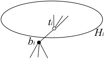 Figure 41
 Figure 51
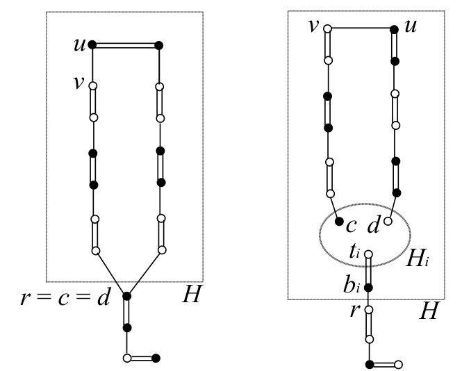 Figure 61
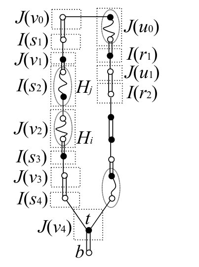 Figure 72
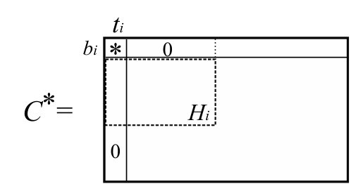 Figure 1
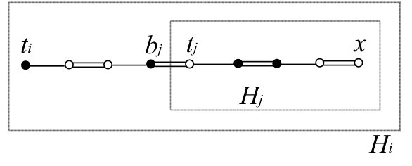 Figure 4
 Figure 5
 Figure 6
 Figure 9
 Figure 10
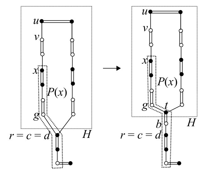 Figure 11
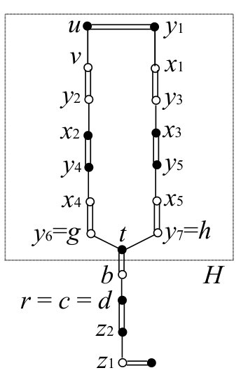 Figure 12
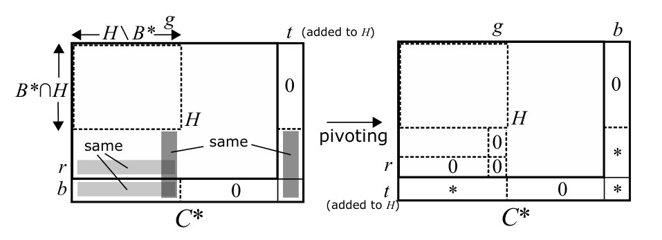 Figure 13
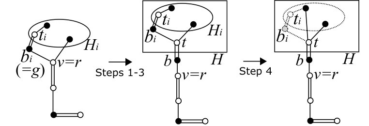 Figure 15
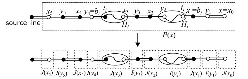 Figure 16
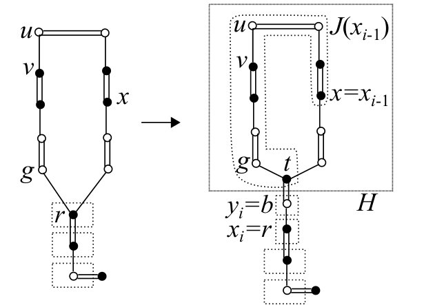 Figure 18
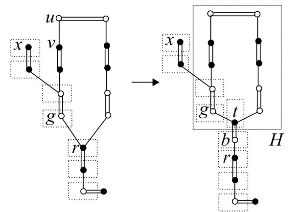 Figure 19
 Figure 20
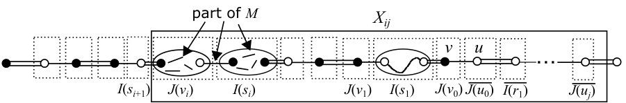 Figure 21
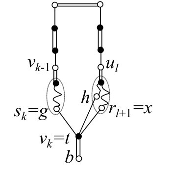 Figure 22
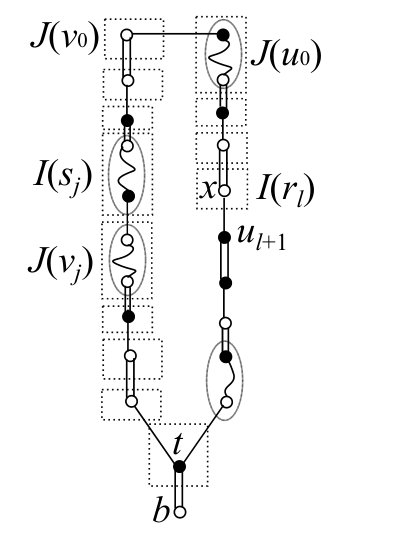 Figure 23
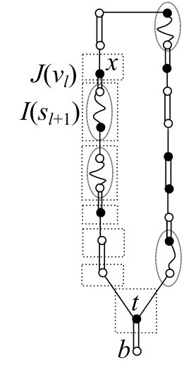 Figure 24
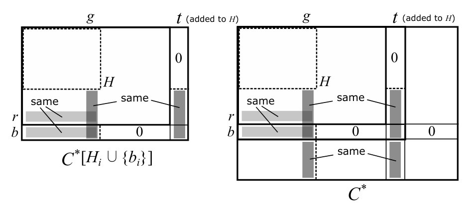 Figure 30
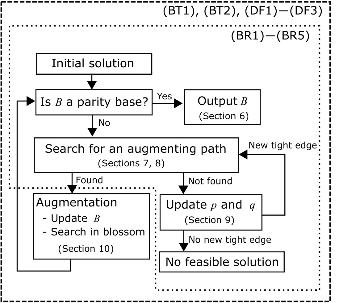 Figure 31
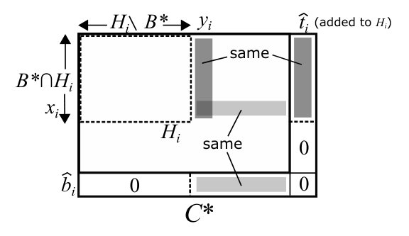 Figure 32
Peer Reviews
No public reviews on file for this paper yet. If you reviewed it on a platform where reviews are public (OpenReview, ICLR, NeurIPS, ICML), you can paste yours below so the community can read it here.
Videos
No videos yet. Explain this paper in a talk, walkthrough, or lecture? Add one.
Taxonomy
TopicsComplexity and Algorithms in Graphs · Advanced Graph Theory Research · Optimization and Search Problems
A Weighted Linear Matroid Parity Algorithm††thanks:
A preliminary version of this paper has appeared in Proceedings of the 49th Annual ACM Symposium on Theory of Computing (STOC 2017), pp. 264–276.
Satoru Iwata Department of Mathematical Informatics, University of Tokyo, Tokyo 113-8656, Japan. E-mail: [email protected]
Yusuke Kobayashi Research Institute for Mathematical Sciences, Kyoto University, Kyoto, 606-8502, Japan. E-mail: [email protected]
Abstract
The matroid parity (or matroid matching) problem, introduced as a common generalization of matching and matroid intersection problems, is so general that it requires an exponential number of oracle calls. Nevertheless, Lovász (1980) showed that this problem admits a min-max formula and a polynomial algorithm for linearly represented matroids. Since then efficient algorithms have been developed for the linear matroid parity problem.
In this paper, we present a combinatorial, deterministic, polynomial-time algorithm for the weighted linear matroid parity problem. The algorithm builds on a polynomial matrix formulation using Pfaffian and adopts a primal-dual approach based on the augmenting path algorithm of Gabow and Stallmann (1986) for the unweighted problem.
1 Introduction
The matroid parity problem [22] (also known as the matchoid problem [20] or the matroid matching problem [24]) was introduced as a common generalization of matching and matroid intersection problems. In the general case, it requires an exponential number of independence oracle calls [19, 26], and a PTAS has been developed only recently [23]. Nevertheless, Lovász [24, 26, 27] showed that the problem admits a min-max theorem for linear matroids and presented a polynomial algorithm that is applicable if the matroid in question is represented by a matrix.
Since then, efficient combinatorial algorithms have been developed for this linear matroid parity problem [12, 33, 34]. Gabow and Stallmann [12] developed an augmenting path algorithm with the aid of a linear algebraic trick, which was later extended to the linear delta-matroid parity problem [14]. Orlin and Vande Vate [34] provided an algorithm that solves this problem by repeatedly solving matroid intersection problems coming from the min-max theorem. Later, Orlin [33] improved the running time bound of this algorithm. The current best deterministic running time bound due to [12, 33] is , where is the cardinality of the ground set, is the rank of the linear matroid, and is the matrix multiplication exponent, which is at most . These combinatorial algorithms, however, tend to be complicated.
An alternative approach that leads to simpler randomized algorithms is based on an algebraic method. This is originated by Lovász [25], who formulated the linear matroid parity problem as rank computation of a skew-symmetric matrix that contains independent parameters. Substituting randomly generated numbers to these parameters enables us to compute the optimal value with high probability. A straightforward adaptation of this approach requires iterations to find an optimal solution. Cheung, Lau, and Leung [3] have improved this algorithm to run in time, extending the techniques of Harvey [16] developed for matching and matroid intersection.
While matching and matroid intersection algorithms [7, 9] have been successfully extended to their weighted version [8, 10, 18, 21], no polynomial algorithms have been known for the weighted linear matroid parity problem for more than three decades. Camerini, Galbiati, and Maffioli [2] developed a random pseudopolynomial algorithm for the weighted linear matroid parity problem by introducing a polynomial matrix formulation that extends the matrix formulation of Lovász [25]. This algorithm was later improved by Cheung, Lau, and Leung [3]. The resulting complexity, however, remained pseudopolynomial. Tong, Lawler, and Vazirani [39] observed that the weighted matroid parity problem on gammoids can be solved in polynomial time by reduction to the weighted matching problem. As a relaxation of the matroid matching polytope, Vande Vate [41] introduced the fractional matroid matching polytope. Gijswijt and Pap [15] devised a polynomial algorithm for optimizing linear functions over this polytope. The polytope was shown to be half-integral, and the algorithm does not necessarily yield an integral solution.
This paper presents a combinatorial, deterministic, polynomial-time algorithm for the weighted linear matroid parity problem. To do so, we combine algebraic approach and augmenting path technique together with the use of node potentials. The algorithm builds on a polynomial matrix formulation, which naturally extends the one discussed in [13] for the unweighted problem. The algorithm employs a modification of the augmenting path search procedure for the unweighted problem by Gabow and Stallmann [12]. It adopts a primal-dual approach without writing an explicit LP description. The correctness proof for the optimality is based on the idea of combinatorial relaxation for polynomial matrices due to Murota [31]. The algorithm is shown to require arithmetic operations. This leads to a strongly polynomial algorithm for linear matroids represented over a finite field. For linear matroids represented over the rational field, one can exploit our algorithm to solve the problem in polynomial time.
Independently of the present work, Gyula Pap has obtained another combinatorial, deterministic, polynomial-time algorithm for the weighted linear matroid parity problem based on a different approach.
The matroid matching theory of Lovász [27] in fact deals with a more general class of matroids that enjoy the double circuit property. Dress and Lovász [6] showed that algebraic matroids satisfy this property. Subsequently, Hochstättler and Kern [17] showed the same phenomenon for pseudomodular matroids. The min-max theorem follows for this class of matroids. To design a polynomial algorithm, however, one has to establish how to represent those matroids in a compact manner. Extending this approach to the weighted problem is left for possible future investigation.
The linear matroid parity problem finds various applications: structural solvability analysis of passive electric networks [30], pinning down planar skeleton structures [28], and maximum genus cellular embedding of graphs [11]. We describe below two interesting applications of the weighted matroid parity problem in combinatorial optimization.
A -path in a graph is a path between two distinct vertices in the terminal set . Mader [29] showed a min-max characterization of the maximum number of openly disjoint -paths. The problem can be equivalently formulated in terms of -paths, where is a partition of and an -path is a -path between two different components of . Lovász [27] formulated the problem as a matroid matching problem and showed that one can find a maximum number of disjoint -paths in polynomial time. Schrijver [37] has described a more direct reduction to the linear matroid parity problem.
The disjoint -paths problem has been extended to path packing problems in group-labeled graphs [4, 5, 35]. Tanigawa and Yamaguchi [38] have shown that these problems also reduce to the matroid matching problem with double circuit property. Yamaguchi [42] clarifies a characterization of the groups for which those problems reduce to the linear matroid parity problem.
As a weighted version of the disjoint -paths problem, it is quite natural to think of finding disjoint -paths of minimum total length. It is not immediately clear that this problem reduces to the weighted linear matroid parity problem. A recent paper of Yamaguchi [43] clarifies that this is indeed the case. He also shows that the reduction results on the path packing problems on group-labeled graphs also extend to the weighted version.
The weighted linear matroid parity is also useful in the design of approximation algorithms. Prömel and Steger [36] provided an approximation algorithm for the Steiner tree problem. Given an instance of the Steiner tree problem, construct a hypergraph on the terminal set such that each hyperedge corresponds to a terminal subset of cardinality at most three and regard the shortest length of a Steiner tree for the terminal subset as the cost of the hyperedge. The problem of finding a minimum cost spanning hypertree in the resulting hypergraph can be converted to the problem of finding a minimum spanning tree in a 3-uniform hypergraph, which is a special case of the weighted parity problem for graphic matroids. The minimum spanning hypertree thus obtained costs at most 5/3 of the optimal value of the original Steiner tree problem, and one can construct a Steiner tree from the spanning hypertree without increasing the cost. Thus they gave a 5/3-approximation algorithm for the Steiner tree problem via weighted linear matroid parity. This is a very interesting approach that suggests further use of weighted linear matroid parity in the design of approximation algorithms, even though the performance ratio is larger than the current best one for the Steiner tree problem [1].
2 The Minimum-Weight Parity Base Problem
Let be a matrix of row-full rank over an arbitrary field with row set and column set . Assume that both and are even. The column set is partitioned into pairs, called lines. Each has its mate such that is a line. We denote by the set of lines, and suppose that each line has a weight .
The linear dependence of the column vectors naturally defines a matroid on . Let denote its base family. A base is called a parity base if it consists of lines. As a weighted version of the linear matroid parity problem, we will consider the problem of finding a parity base of minimum weight, where the weight of a parity base is the sum of the weights of lines in it. We denote the optimal value by . This problem generalizes finding a minimum-weight perfect matching in graphs and a minimum-weight common base of a pair of linear matroids on the same ground set.
As another weighted version of the matroid parity problem, one can think of finding a matching (independent parity set) of maximum weight. This problem can be easily reduced to the minimum-weight parity base problem.
Associated with the minimum-weight parity base problem, we consider a skew-symmetric polynomial matrix in variable defined by
[TABLE]
where is a block-diagonal matrix in which each block is a skew-symmetric polynomial matrix corresponding to a line . Assume that the coefficients are independent parameters (or indeterminates).
For a skew-symmetric matrix whose rows and columns are indexed by , the support graph of is the graph with edge set . We denote by the Pfaffian of , which is defined as follows:
[TABLE]
where the sum is taken over all perfect matchings in and takes in a suitable manner, see [28]. It is well-known that and for any square matrix .
We have the following lemma that associates the optimal value of the minimum-weight parity base problem with .
Lemma 2.1**.**
The optimal value of the minimum-weight parity base problem is given by
[TABLE]
In particular, if (i.e., ), then there is no parity base.
Proof.
We split into and such that
[TABLE]
The row and column sets of these skew-symmetric matrices are indexed by . By [32, Lemma 7.3.20], we have
[TABLE]
where each sign is determined by the choice of , is the principal submatrix of whose rows and columns are both indexed by , and is defined in a similar way. One can see that if and only if (or, equivalently ) is a union of lines. One can also see for that if and only if is nonsingular, which means that is a base of . Thus, we have
[TABLE]
where the sum is taken over all parity bases . Note that no term is canceled out in the summation, because each term contains a distinct set of independent parameters. For a parity base , we have
[TABLE]
which implies that the minimum weight of a parity base is . ∎
Note that Lemma 2.1 does not immediately lead to a (randomized) polynomial-time algorithm for the minimum weight parity base problem. This is because computing the degree of the Pfaffian of a skew-symmetric polynomial matrix is not so easy. Indeed, the algorithms in [2, 3] for the weighted linear matroid parity problem compute the degree of the Pfaffian of another skew-symmetric polynomial matrix, which results in pseudopolynomial complexity.
3 Algorithm Outline
In this section, we describe the outline of our algorithm for solving the minimum-weight parity base problem.
We regard the column set as a vertex set. The algorithm works on a vertex set that includes some new vertices generated during the execution. The algorithm keeps a nested (laminar) collection of vertex subsets of such that is a union of lines for each . The indices satisfy that, for any two members with , either or holds. Each member of is called a blossom. The algorithm maintains a potential and a nonnegative variable , which are collectively called dual variables.
We note that although and are called dual variables, they do not correspond to dual variables of an LP-relaxation of the minimum-weight parity base problem. Indeed, this paper presents neither an LP-formulation nor a min-max formula for the minimum-weight parity base problem, explicitly. We will show instead that one can obtain a parity base that admits feasible dual variables and , which provide a certificate for the optimality of .
The algorithm starts with splitting the weight into and for each line , i.e., . Then it executes the greedy algorithm for finding a base with minimum value of . If is a parity base, then is obviously a minimum-weight parity base. Otherwise, there exists a line in which exactly one of its two vertices belongs to . Such a line is called a source line and each vertex in a source line is called a source vertex. A line that is not a source line is called a normal line.
The algorithm initializes and proceeds iterations of primal and dual updates, keeping dual feasibility. In each iteration, the algorithm applies the breadth-first search to find an augmenting path. In the meantime, the algorithm sometimes detects a new blossom and adds it to . If an augmenting path is found, the algorithm updates along . This will reduce the number of source lines by two. If the search procedure terminates without finding an augmenting path, the algorithm updates the dual variables to create new tight edges. The algorithm repeats this process until becomes a parity base. Then is a minimum-weight parity base. See Fig. 1 for a flowchart of our algorithm.
The rest of this paper is organized as follows.
In Section 4, we introduce new vertices and operations attached to blossoms. We describe some properties of blossoms kept in the algorithm, which we denote (BT1) and (BT2).
The feasibility of the dual variables is defined in Section 5. The dual feasibility is denoted by (DF1)–(DF3). We also describe several properties of feasible dual variables that are used in other sections.
In Section 6, we show that a parity base that admits feasible dual variables attains the minimum weight. The proof is based on the polynomial matrix formulation of the minimum-weight parity base problem given in Section 2. Combining this with some properties of the dual variables and the duality of the maximum-weight matching problem, we show the optimality of such a parity base.
In Section 7, we describe a search procedure for an augmenting path. We first define an augmenting path, and then we describe our search procedure. Roughly, our procedure finds a part of the augmenting path outside the blossoms. The routing in each blossom is determined by a prescribed vertex set that satisfies some conditions, which we denote (BR1)–(BR5). Note that the search procedure may create new blossoms.
The validity of the procedure is shown in Section 8. We show that the output of the procedure is an augmenting path by using the properties (BR1)–(BR5) of the routing in each blossom. We also show that creating a new blossom does not violate the conditions (BT1), (BT2), (DF1)–(DF3), and (BR1)–(BR5).
In Section 9, we describe how to update the dual variables when the search procedure terminates without finding an augmenting path. We obtain new tight edges by updating the dual variables, and repeat the search procedure. We also show that if we cannot obtain new tight edges, then the instance has no feasible solution, i.e., there is no parity base.
If the search procedure succeeds in finding an augmenting path , the algorithm updates the base along . The details of this process are presented in Section 10. Basically, we replace the base with the symmetric difference of and . In addition, since there exist new vertices corresponding to the blossoms, we update them carefully to keep the conditions (BT1), (BT2), and (DF1)–(DF3). In order to define a new routing in each blossom, we apply the search procedure in each blossom, which enables us to keep the conditions (BR1)–(BR5).
Finally, in Section 11, we describe the entire algorithm and analyze its running time. We show that our algorithm solves the minimum-weight parity base problem in time when is a finite field of fixed order. When , it is not obvious that a direct application of our algorithm runs in polynomial time. However, we show that the minimum-weight parity base problem over can be solved in polynomial time by applying our algorithm over a sequence of finite fields.
4 Blossoms
In this section, we introduce buds and tips attached to blossoms and construct auxiliary matrices that will be used in the definition of dual feasibility.
Each blossom contains at most one source line. A blossom that contains a source line is called a source blossom. A blossom with no source line is called a normal blossom. Let and denote the sets of source blossoms and normal blossoms, respectively. Then, . Let denote the number of blossoms in .
Each normal blossom has a pair of associated vertices and outside , which are called the bud and the tip of , respectively. The pair is called a dummy line. To simplify the description, we denote and . The vertex set is defined by with . The tip is contained in , whereas the bud is outside . For every with , we have if and only if . Similarly, we have if and only if . Thus, each normal blossom is of odd cardinality. The algorithm keeps a subset such that and for each . It also keeps for distinct and for each . This implies that , where , and hence .
Recall that is the row set of . The fundamental cocircuit matrix with respect to a base is a matrix with row set and column set obtained by . In other words, is obtained from by identifying and , applying row transformations, and changing the ordering of columns. For a subset , we have if and only if is nonsingular. Here, denotes the symmetric difference. Then the following lemma characterizes the fundamental cocircuit matrix with respect to .
Lemma 4.1**.**
Suppose that is in the form of with being nonsingular. Then
[TABLE]
is the fundamental cocircuit matrix with respect to .
Proof.
In order to obtain the fundamental cocircuit matrix with respect to , we apply row elementary transformations to so that the columns corresponding to form the identity matrix. Hence, the obtained matrix is
[TABLE]
which shows that is the fundamental cocircuit matrix with respect to . ∎
This operation converting to is called pivoting around . We have the following property on the nonsingularity of their submatrices.
Lemma 4.2**.**
Let and be the fundamental cocircuit matrices with respect to and , respectively. Then, for any , is nonsingular if and only if is nonsingular.
Proof.
Consider the matrix whose column set is equal to . Then, is nonsingular if and only if the columns of indexed by form a nonsingular matrix. This is equivalent to that the corresponding columns of form a nonsingular matrix, which means that is nonsingular. ∎
The algorithm keeps a matrix whose row and column sets are and , respectively. The matrix is obtained from by attaching additional rows/columns corresponding to , and then pivoting around . Thus we have . In other words, the matrix obtained from by pivoting around contains as a submatrix (see (BT1) below). If the row and column sets of are clear, for a vertex set , we denote .
In our algorithm, the matrix satisfies the following properties.
(BT1)
Let be the matrix obtained from by pivoting around . Then, is the fundamental cocircuit matrix with respect to .
(BT2)
Each normal blossom satisfies the following.
- •
If and , then , for any with , and for any with (see Fig. 2).
- •
If and , then , for any with , and for any with .
5 Dual Feasibility
In this section, we define feasibility of the dual variables and show their properties. Our algorithm for the minimum-weight parity base problem is designed so that it keeps the dual feasibility.
Recall that a potential , and a nonnegative variable are called dual variables. A blossom is said to be positive if . For distinct vertices and for , we say that a pair crosses if . For distinct , we denote by the set of indices such that crosses . We introduce the set of ordered vertex pairs defined by
[TABLE]
For distinct , we define
[TABLE]
The dual variables are called feasible with respect to and if they satisfy the following.
(DF1)
for every line .
(DF2)
for every .
(DF3)
for every and with .
If no confusion may arise, we omit and when we discuss dual feasibility.
Note that if , then corresponds to the nonzero entries of , which shows that holds for . This implies that (DF2) holds if is a base minimizing , because for any . We also note that (DF3) holds if . Therefore, and are feasible if satisfies (DF1), , and minimizes in . This ensures that the initial setting of the algorithm satisfies the dual feasibility.
We now show some properties of feasible dual variables.
Lemma 5.1**.**
Suppose that and are feasible dual variables. Let be a vertex subset such that is nonsingular. Then, we have
[TABLE]
Proof.
Since is nonsingular, there exists a perfect matching between and such that , , and for . The dual feasibility implies that for . Combining these inequalities, we obtain
[TABLE]
If is odd, there exists an index such that , which shows that the coefficient of in the right hand side of (1) is at least . This completes the proof ∎
We now consider the tightness of the inequality in Lemma 5.1. Let be the undirected graph with vertex set and edge set , where we regard as a set of unordered pairs. An edge with and is said to be tight if . We say that a matching is consistent with a blossom if at most one edge in crosses . We say that a matching is tight if every edge of is tight and is consistent with every positive blossom . As the proof of Lemma 5.1 clarifies, if there exists a tight perfect matching in the subgraph of induced by , then the inequality of Lemma 5.1 is tight. Furthermore, in such a case, every perfect matching in must be tight, which is stated as follows.
Lemma 5.2**.**
For a vertex set , if has a tight perfect matching, then any perfect matching in is tight.
When for some , one can delete from without violating the dual feasibility. In fact, removing such a source blossom does not affect the dual feasibility, (BT1), and (BT2). If is a normal blossom, then apply the pivoting operation around to , remove and from , and remove from . This process is referred to as .
Lemma 5.3**.**
If for some , the dual variables remain feasible and (BT1) and (BT2) hold after is executed.
Proof.
We only consider the case when and , since we can deal with the case of and in the same way. Let be the original matrix and be the matrix obtained after is executed. Let (resp. ) be the ordered vertex pairs corresponding to the nonzero entries of (resp. ).
Suppose that and are feasible with respect to . In order to show that and are feasible with respect to , it suffices to consider (DF2), since (DF1) and (DF3) are obvious. Suppose that . If , then by the dual feasibility with respect to . Otherwise, we have and . By Lemma 4.1, , and hence and imply that and . Then, by the dual feasibility with respect to , we obtain
[TABLE]
Furthermore, we have by (DF3) and . By combining these inequalities, we obtain . This shows that (DF2) holds with respect to .
By the definition of , it is obvious that satisfies (BT1).
To show (BT2), let be a normal blossom that is different from . Suppose that and . we consider the following cases, separately.
- •
If , then for any . In particular, .
- •
If , then for any . In particular, .
- •
If , then we have that and .
In every case, we have that for any , and for any . Therefore, , for any with , and for any with . We can deal with the case when and in a similar way. This shows that satisfies (BT2). ∎
6 Optimality
In this section, we show that if we obtain a parity base and feasible dual variables and , then is a minimum-weight parity base.
Note again that although and are called dual variables, they do not correspond to dual variables of an LP-relaxation of the minimum-weight parity base problem. Our optimality proof is based on the algebraic formulation of the problem (Lemma 2.1) and the duality of the maximum-weight matching problem.
Theorem 6.1**.**
If is a parity base and there exist feasible dual variables and , then is a minimum-weight parity base.
Proof.
Since the optimal value of the minimum-weight parity base problem is represented with as shown in Lemma 2.1, we evaluate the value of , assuming that we have a parity base and feasible dual variables and .
Recall that is transformed to by applying row transformations and column permutations, where is the fundamental cocircuit matrix with respect to the base obtained by . Note that the identity submatrix gives a one to one correspondence between and , and the row set of can be regarded as . We now apply the same row transformations and column permutations to , and then apply also the corresponding column transformations and row permutations to obtain a skew-symmetric polynomial matrix , that is,
[TABLE]
where is a skew-symmetric matrix obtained from by applying row and column permutations simultaneously. Note that , where the sign is determined by the ordering of .
We now consider the following skew-symmetric matrix:
[TABLE]
Here, the row and column sets of are both indexed by , where is the row set of , which can be identified with . Then, we have the following claim.
Claim 6.2**.**
It holds that .
Proof.
Since satisfies (BT1), we can obtain \left(\begin{array}[]{c|c|c}O&X&I\\ \hline\cr I&C&O\end{array}\right) from \left(\begin{array}[]{c|c|c}O&\lx@intercol\hfil\hfil\lx@intercol\\ \cline{1-1}\cr I&\lx@intercol\hfil\raisebox{7.0pt}[0.0pt][0.0pt]{\ C^{*}}\hfil\lx@intercol\end{array}\right) by applying elementary row transformations, where is some matrix. Here, the row and column sets are and , respectively. We apply the same row transformations and their corresponding column transformations to . Then, we obtain the following matrix:
[TABLE]
and hence . Since , we have that
[TABLE]
which completes the proof. ∎
In what follows, we evaluate . Construct a graph with edge set . Each edge has a weight . Then it can be easily seen by the definition of Pfaffian that the maximum weight of a perfect matching in is at least . Let us recall that the dual linear program of the maximum-weight perfect matching problem on is formulated as follows.
[TABLE]
where \Omega=\{Z\mid Z\subseteq W^{*},\,\mbox{|Z|: odd},|Z|\geq 3\} and (see, e.g., [37, Theorem 25.1]). In what follows, we construct a feasible solution of this linear program. The objective value provides an upper bound on the maximum weight of a perfect matching in , and consequently serves as an upper bound on .
Since can be identified with , we can naturally define a bijection between and . We define by
[TABLE]
For each , we introduce and set (see Fig. 3). Since is of odd cardinality and there is no source line in , we see that
[TABLE]
is odd and . Define for any . We now show the following claim.
Claim 6.3**.**
The dual variables and defined as above form a feasible solution of the linear program (6).
Proof.
Suppose that . If and , then (DF1) shows that , where . Since is even for any , this shows (6). If and , then implies that , and hence , which shows (6) as is even for any .
The remaining case of is when and . That is, it suffices to show that satisfies (6) if . By the definition of , we have , where . By the definition of , we have if and only if , which shows that
[TABLE]
Since , by (DF2), we have
[TABLE]
Thus, we obtain
[TABLE]
which shows that satisfies (6). ∎
The objective value of this feasible solution is
[TABLE]
where the first equality follows from the definition of , the second one follows from the definition of and (DF3), and the third one follows from (DF1). By the weak duality of the maximum-weight matching problem, we have
[TABLE]
On the other hand, Lemma 2.1 shows that any parity base satisfies that
[TABLE]
Combining (3)–(5), we have , which means is a minimum-weight parity base by Lemma 2.1. ∎
7 Finding an Augmenting Path
In this section, we define an augmenting path and present a procedure for finding one. The validity of our procedure is shown in Section 8.
Suppose we are given , , , , and feasible dual variables and . Let be the set of tight edges, i.e., . Our procedure works primarily on the undirected graph , where we ignore the ordering of the vertices when we regard or as an edge set. For a vertex set , denotes the subgraph of induced by . For , define as
[TABLE]
Here, is regarded as if . This definition shows that we can ignore when we consider edges in (or ) connecting and .
Roughly, our procedure finds a part of the augmenting path outside the blossoms. The routing in each blossom is determined by a prescribed vertex set for , where . For any and for any , the prescribed vertex set is assumed to satisfy the following.
(BR1)
.
(BR2)
If , then consists of lines, dummy lines, and the tip . If , then consists of lines, dummy lines, and a source vertex.
(BR3)
For any with and , it holds that .
See Fig. 4 for an example of . We sometimes regard as a sequence of vertices, and in such a case, the last two vertices are . We also suppose that the first vertex of is if and the unique source vertex in if . Each blossom is assigned a total order among all the vertices in . In the procedure, keeps additional properties which will be described in Section 8.1.
We say that a vertex set is an augmenting path if it satisfies the following properties.
(AP1)
consists of normal lines, dummy lines, and two vertices from distinct source lines.
(AP2)
For each , either or for some .
(AP3)
has a unique tight perfect matching.
By (AP1), (AP2), and (BR2), we have the following observation.
Observation 7.1**.**
For an augmenting path and for each with , it holds that .
In the rest of this section, we describe how to find an augmenting path. Section 7.1 is devoted to the search procedure, which calls two procedures: and . The details of these procedures are described in Sections 7.2 and 7.3, respectively. In Section 7.4, we show that the procedure keeps some conditions.
7.1 Search Procedure
In this subsection, we describe a procedure for searching for an augmenting path. The procedure performs the breadth-first search using a queue to grow paths from source vertices. A vertex is labeled and put into the queue when it is reached by the search. The procedure picks the first labeled element from the queue, and examines its neighbors. A linear order is defined on the labeled vertex set so that means is labeled prior to .
For each , we define if there exists a maximal blossom such that is a normal blossom with , and define if there exists a maximal blossom such that is a source blossom with . If such a blossom does not exist, then it is called single and we denote . The procedure also labels some blossoms with or , which will be used later for modifying dual variables. With each labeled vertex , the procedure associates a path and its subpath , where a path is a sequence of vertices. The first vertex of is a labeled vertex in a source line and the last one is . The reverse path of is denoted by . For a path and a vertex in , we denote by the subsequence of after (not including ). We sometimes identify a path with its vertex set. When an unlabeled vertex is examined in the procedure, we assign a vertex and a path . Roughly, is a neighbor of such that is examined when we pick up from the queue. Paths and , where is an unlabeled vertex and is a labeled vertex, are used to decompose a search path as we will see in Lemma 8.1 later. Roughly, and represent “fractions” of the search path containing and , respectively. The procedure is described as follows.
Procedure
Step 0:
Initialize the objects so that the queue is empty, every vertex is unlabeled, and every blossom is unlabeled.
Step 1:
While there exists an unlabeled single vertex in a source line, label with and put into the queue. While there exists a source line such that and is adjacent to in , add a new source blossom to , label with , and define and . While there exists an unlabeled maximal source blossom , label with and do the following: for each vertex in the order of , label with and put into the queue.
Step 2:
If the queue is empty, then return and terminate the procedure (see Section 9). Otherwise, remove the first element from the queue.
Step 3:
While there exists a labeled vertex adjacent to in with , choose such that is minimum with respect to and do the following (3-1) and (3-2) (see Fig. 5).
(3-1)
If the first elements in and in belong to different source lines, then return as an augmenting path.
(3-2)
Otherwise, apply to add a new blossom to .
Step 4:
While there exists an unlabeled vertex adjacent to in with such that is not assigned, do the following (4-1)–(4-3).
(4-1)
If , then label with and , set and , and put into the queue (see Fig. 8). Furthermore, if , then apply .
(4-2)
If for some and , then apply (see Fig. 8).
(4-3)
If for some and , then choose with that is minimum with respect to , and do the following.111Such always exists, because satisfies the condition. Label with , label with and , and put into the queue. For each unlabeled vertex , set and (see Fig. 8).
Step 5:
Go back to Step 2.
7.2 Creating a Blossom
In this subsection, we describe procedure that creates a new blossom, which is called in Steps (3-2) and (4-1) of .
Procedure
Step 1:
Let be the last vertex in such that contains a vertex in . Let be the last vertex in contained in . Note that . If , then define and . If , then define and let be the last vertex in not contained in if exists. See Fig. 9 for an example.
Step 2:
If contains no source line, then define to be the vertex subsequent to in , introduce new vertices and , namely , and add to , namely . Update , , and as follows (see Fig. 10).
- •
If and , then , , for , for , for , for , and .
- •
If and , then , , for , for , for , for , and .
- •
Apply the pivoting operation around to , namely , and update accordingly.
Step 3:
If contains no source line, then for each labeled vertex with , replace by . Label with and , and extend the ordering of the labeled vertices so that is just after , i.e., and no element is between and . For each vertex with , update as . Set and (see Fig. 11).
Step 4:
For each unlabeled vertex , label as follows.
- (i)
If and , then . 2. (ii)
If and , then . 3. (iii)
If for some labeled with such that and , then . 4. (iv)
If for some labeled with such that and , then . 5. (v)
If for some labeled with such that and , then . 6. (vi)
If for some labeled with such that and , then .
Define and put into the queue (see Fig. 12). Here, we choose the vertices in the ordering such that the following conditions hold.
- •
For two unlabeled vertices , if , then we choose prior to .
- •
For two unlabeled vertices , if , , and , then we choose prior to .
- •
If holds, then no element is chosen between and , where is the vertex subsequent to in . Note that this condition makes sense only when or corresponds to a blossom labeled with .
Step 5:
Label with . Define for each if contains no source line, and define for each if contains a source line. Define by the ordering of the labeled vertices in . Add to with regarding and , if exist, as the bud and the tip of , respectively, and update , , , , and for , accordingly.
We note that, for any , if (resp. ) is defined, then it is equal to either or (resp. either or ) for some . In particular, the last element of and the first element of are . We also note that and are not used in the procedure explicitly, but we introduce them to show the validity of the procedure.
7.3 Grafting a Blossom
In this subsection, we describe that replaces a blossom with another blossom, which is called in Step (4-2) of . See Fig. 13 for an illustration.
Procedure
Step 1:
Set , where is a normal blossom. Introduce new vertices and in the same say as Step 2 of with and , add to , and apply the pivoting operation around to . Label with and , and extend the ordering of the labeled vertices so that is just after , i.e., and no element is between and . Set and .
Step 2:
For each vertex in the order of , label with and , and put into the queue.
Step 3:
Label with . Define for each . Define by the ordering of the labeled vertices in . Add to with regarding and as the bud and the tip of , respectively, and update , , , and for , accordingly.
Step 4:
Set and modify the dual variables by , ,
[TABLE]
Apply to delete from , and set . For each vertex , delete and from , , and .
We note that Step 4 of is executed to keep the condition for distinct .
7.4 Basic Properties
For better understanding of the pivoting operations in and , we give several lemmas in this subsection. Then, we show that the conditions (BT1), (BT2), and (DF1)–(DF3) hold in the search procedure.
Lemma 7.2**.**
Suppose that or Steps 1–3 of have created a new blossom containing no source line. Then the following conditions hold after the pivoting operation:
- •
* and satisfy the conditions in (BT2),*
- •
there is no edge in between and , and
- •
there is no edge in between and .
Proof.
To show the properties, we use the notation , , and to represent the objects after the pivoting operation, whereas , , , and represent those before the pivoting operation. We only consider the case when and as the other case can be dealt with in a similar way.
In Step 2 of (or Step 1 of ), we have , and hence . Since for any , we have for any with . Similarly, since for any , we have for any with . Thus, and satisfy the conditions in (BT2).
Since and for any , we have for any by Lemma 4.1. Thus, there is no edge in between and . Similarly, since and for any , we have for any by Lemma 4.1. Thus, there is no edge in between and . ∎
The following lemma shows how creating a blossom affects the edges in .
Lemma 7.3**.**
Suppose that or Steps 1–3 of have created a new blossom containing no source line, and let (resp. ) be the tight edge set before (resp. after) the execution of or Steps 1–3 of . If , then (i) , or (ii) exactly one of , say , is contained in , and .
Proof.
Suppose that . By Lemma 4.1, we have only when or holds before the pivoting operation in Step 2 of (or Step 1 of ). This shows that exactly one of , say , is contained in , and that holds before (or ).
Suppose that . In this case, if holds before (or ) and , then we have
[TABLE]
Furthermore, we have by a simple counting argument. Combining these inequalities, we see that all the inequalities above must be tight. Thus, we have . The same argument can be applied to the case when . ∎
The proof of this lemma implies the following result.
Corollary 7.4**.**
Suppose that or Steps 1–3 of have created a new blossom containing no source line, and let (resp. ) be the edge set before (resp. after) the execution of or Steps 1–3 of . If , then (i) , or (ii) exactly one of , say , is contained in , and .
The following lemma shows that Step 4 of roughly replaces edges incident to with ones incident to .
Lemma 7.5**.**
Suppose that is executed for some positive blossom in . Then, we have the following.
- •
* does not affect the edges in that are not incident to .*
- •
If after , then or before .
- •
If after , then or before .
- •
If before with , then after .
Proof.
Since is the only edge in connecting and , and are the only edges in incident to just before . Thus, the first property holds. By Lemma 4.2, after if and only if is nonsingular before , which shows the second property. Then, by the dual feasibility, we obtain the third property. If before , then before by the dual feasibility, and hence is nonsingular. Thus, after . ∎
We can also see that creating a new blossom does not violate the dual feasibility as follows.
Lemma 7.6**.**
Suppose that the dual variables are feasible before or Steps 1–3 of , which create a new blossom . Then, the dual variables remain feasible after or Steps 1–3 of .
Proof.
We use , , , , , and to represent the objects after (or Steps 1–3 of ), whereas , , , , , and represent the objects before (or Steps 1–3 of ). We only consider the case when and , as the other case can be dealt with in a similar way.
Since there is an edge in between and , we have , and hence
[TABLE]
By the definition of , we have the following.
- •
If for , then and . Thus, we have
[TABLE]
by (6) and the dual feasibility before (or Steps 1–3 of ).
- •
If for , then and . Thus, we have
[TABLE]
by (6), the dual feasibility before (or Steps 1–3 of ), and .
- •
If for and , then , , and by Corollary 7.4. Thus, we have
[TABLE]
by the dual feasibility before (or Steps 1–3 of ).
These facts show that and are feasible with respect to . ∎
It is obvious that creating a new blossom does not violate (BT1). Thus, by Lemmas 5.3, 7.2, and 7.6, we see that the procedure Search keeps the conditions (BT1), (BT2), and (DF1)–(DF3).
8 Validity
This section is devoted to the validity proof of the procedures described in Section 7. In Section 8.1, we introduce properties (BR4) and (BR5) of the routing in blossoms. The procedures are designed so that they keep the conditions (BR1)–(BR5). Assuming these conditions, we show in Section 8.2 that a nonempty output of is indeed an augmenting path. In Section 8.3, we show that these conditions hold during the procedure.
8.1 Properties of Routings in Blossoms
In this subsection, we introduce properties (BR4) and (BR5) of kept in the procedure. Recall that, for ,
[TABLE]
In addition to (BR1)–(BR3), we assume that satisfies the following (BR4) and (BR5) for any and .
(BR4)
has a unique tight perfect matching.
(BR5)
If , then we have the following. Suppose that satisfies that for any , , and for any positive blossom . Then, has no tight perfect matching.
Here, we suppose that has a unique tight perfect matching to simplify the description.
We now explain roles of (BR4) and (BR5). These conditions are used to show that the output in Step (3-1) of satisfies (AP3), i.e., has a unique tight perfect matching. We will show that the obtained path can be decomposed into subsequences, and each subsequence consists of a singleton or a set for some (see Lemma 8.1). Our aim is to show that if has a tight perfect matching, then is the only vertex in that is matched with a vertex outside . This is guaranteed by (BR5), where means the set of vertices that are matched with vertices outside . Then, (BR4) assures that there exists a unique perfect matching covering except .
8.2 Finding an Augmenting Path
This subsection is devoted to the validity of Step (3-1) of . We first show the following lemma.
Lemma 8.1**.**
In each step of , for any labeled vertex , is decomposed as
[TABLE]
with such that, for each ,
(PD0)
* is equal to either or for some , and is equal to either or for some positive blossom ,*
(PD1)
* is adjacent to in ,*
(PD2)
the first element of and the last element of form a line or a dummy line,
(PD3)
any labeled vertex with is not adjacent to in , and
(PD4)
* is not adjacent to in . Furthermore, if , then is not adjacent to in .*
See Fig. 14 for an example of the decomposition.
Proof.
The procedure naturally defines the decomposition
[TABLE]
It suffices to show that and do not violate the conditions (PD0)–(PD4), since we can easily see that the other operations do not violate them.
We first consider the case when is applied to obtain a new blossom . In , is updated or defined as , , or . Let (resp. ) be the tight edge sets before (resp. after) the execution of that adds to .
Suppose that is defined by , where and . In this case, (PD0), (PD1), and (PD2) are trivial. We now consider (PD3). Since satisfies (PD3), in order to show that any labeled vertex with is not adjacent to in , it suffices to consider the case when , , and (see Fig. 15). Assume to the contrary that is adjacent to in . Since is not adjacent to in by the procedure, Lemma 7.3 shows that . This contradicts that and the definition of . To show (PD4), it suffices to consider the case when . In this case, since is not adjacent to in by Lemma 7.2, satisfies (PD4).
Suppose that is updated as or , where and (see Fig. 16 for an example). In this case, (PD0), (PD1), and (PD2) are trivial. We now consider (PD3). Since (PD3) holds before creating , in order to show that any labeled vertex with is not adjacent to in , it suffices to consider the case when (i) , or (ii) , or (iii) and , or (iv) and by Lemma 7.3. In the first case, if , then , which contradicts that (PD3) holds before creating . In the second case, if , then implies that , which contradicts that and the definition of . If , then implies that , which contradicts that and are labeled. In the third case, implies as (PD3) holds before creating . By the definition of , however, contradicts . In the fourth case, contradicts that and are labeled. By these four cases, we obtain (PD3).
We next consider (PD4). Since (PD4) holds before creating , in order to show that is not adjacent to or in it suffices to consider the case when (i) , or (ii) , or (iii) crosses . In the first case, the claim is obvious. In the second case, if , then , which contradicts that (PD4) holds before creating . In the third case, since and , Lemma 7.3 implies that it suffices to consider the case when and , which contradicts that and are labeled. By these three cases, we obtain (PD4).
We can show that does not violate (PD0)–(PD4) in a similar manner by observing that is updated or defined as or in . We note that in does not affect (PD0)–(PD4) by Lemma 7.5. ∎
Recall that we assume the conditions (BT1), (BT2), (DF1)–(DF3), and (BR1)–(BR5). We are now ready to show the validity of Step (3-1) of .
Lemma 8.2**.**
If returns in Step (3-1), then is an augmenting path.
Proof.
It suffices to show that has a unique tight perfect matching. By Lemma 8.1, and are decomposed as and . For each pair of and , let denote the set of vertices in the subsequence
[TABLE]
of . We intend to show inductively that has a unique tight perfect matching.
We first show that has a unique tight perfect matching. Since and are adjacent in , (PD0) and (BR4) guarantee that has a tight perfect matching. Let be an arbitrary tight perfect matching in , and let be the set of vertices in adjacent to in . If , then it is obvious that . Otherwise, for some . For any positive blossom , since is consistent with by the definition of a tight matching, we have that . Since there are no edges of between and , we have that for any . Furthermore, since there is an edge in connecting each and , we have . Then it follows from (BR5) that has no tight perfect matching unless . This means is the only vertex in adjacent to in . Note that has a unique tight perfect matching by (BR4), which must form a part of . Let be the vertex adjacent to in . Since the vertices in are not adjacent to in , we have if for some (see Fig. 17). By (BR5) again, has no tight perfect matching unless . This means must contain the edge . Note that has a unique tight perfect matching by (BR4), which must form a part of . Thus must be the unique tight perfect matching in .
We now show the statement for general and assuming that the same statement holds if either or is smaller. Suppose that . Then there are no edges of between and by (PD3) of Lemma 8.1. Let be an arbitrary tight perfect matching in , and let be the set of vertices in adjacent to in . Then, by the same argument as above, has no tight perfect matching unless . Thus is the only vertex in matched to in . Since is not adjacent to in by (PD3) and (PD4) of Lemma 8.1, an edge connecting and must belong to . We note that it is the only edge in between and since is tight and is equal to either or for some positive blossom . Let be the vertex adjacent to in . By (BR5), has no tight perfect matching unless (see Fig. 18). This means that contains the edge . Note that each of and has a unique tight perfect matching by (BR4), and so does by induction hypothesis. Therefore, is the unique tight perfect matching in . The case of can be dealt with similarly. Thus, we have seen that has a unique tight perfect matching. ∎
This proof implies the following corollaries.
Corollary 8.3**.**
For any labeled vertex , has a unique tight perfect matching.
Corollary 8.4**.**
If returns , then the unique tight matching in contains exactly one edge connecting and for each with .
8.3 Routing in Blossoms
First, to see that is well-defined for each when we create a new blossom , we observe that every vertex satisfies one of the six cases in Step 4 of . This is because, if for some with , then , and if , , and for some , then by Lemma 7.2.
When we create a new blossom in , for each , clearly satisfies (BR1)–(BR5) by Lemma 7.5. Suppose that a new blossom is created in . For each , defined in also satisfies (BR1)–(BR3). We will show (BR4) and (BR5) in this subsection.
Lemma 8.5**.**
Suppose that creates a new blossom . Then, for each , satisfies (BR4) and (BR5).
Proof.
We only consider the case when contains no source line, since the case with a source line can be dealt with in a similar way. We note that a vertex is adjacent to in before if and only if is adjacent to in after . If , the claim is obvious. We consider the other cases separately.
Case 1. Suppose that was not labeled before is created.
Among six cases in Step 4 of , we consider the cases of (i), (iii), and (v), since the other cases can be dealt with in a similar manner.
By Lemma 8.1, can be decomposed as
[TABLE]
with . In the cases of (i) and (iii), can be decomposed as with , where the first element of is , and hence
[TABLE]
with . Similarly, in the case of (v), can be decomposed as
[TABLE]
Therefore, in the cases of (i), (iii), and (v), we have
[TABLE]
with and (see Fig. 19 for an example).
We now intend to show that satisfies (BR5), that is, has no tight perfect matching if satisfies that for any , , and for any positive blossom . Suppose to the contrary that has a tight perfect matching . Note that , because for any . For each , since either or for some positive blossom , we have . Similarly, . Furthermore, if (resp. ), then (resp. ) is even, and hence there is no edge in between (resp. ) and its outside, because is a tight perfect matching. If , then and contains no edge between and the outside of , which contradicts that has no tight perfect matching by (BR5). Thus, we may assume that . Since implies that there exists no edge in between and the outside of , we can take the largest number such that . We consider the following two cases separately.
Case 1a. Suppose that . In this case, since , there exists an edge in between and . See Fig. 21 for an example. If this edge is incident to , then for some positive blossom and by the procedure, and hence has no tight perfect matching by (BR5), which is a contradiction. Otherwise, since is matched with some vertex , we have , where is as in Step 4 of . This shows that as for any . Since , , and is a tight perfect matching, we have , for some , and each of and has a tight perfect matching. This shows that and by (BR5) and the definition of . Then, we obtain
[TABLE]
Since no element is chosen between and in Step 4 of , we have and , which contradicts that and by Lemma 7.2.
We note that when we apply the same argument to the cases of (ii), (iv), and (vi) by changing the roles of and , we obtain . Then, this contradicts that and .
Case 1b. Suppose that . In this case, since is a tight perfect matching, for , we have and is the only edge in between and the outside of . We can also see that , since for any . We denote by the set of vertices in matched by to the outside of . Since for any and for some , we have , where is the vertex naturally defined by the decomposition of (see Fig. 21). Note that the assumption is used here. Then, for any vertex with , there is no edge in connecting and because of the following:
- •
By (PD3) of Lemma 8.1, is not adjacent to for , because .
- •
By (PD3) of Lemma 8.1, is not adjacent to for , because .
- •
If with , then is not adjacent to by (PD3) of Lemma 8.1.
- •
For , is the only edge in between and its outside, and hence there is no edge is between and .
This shows that . Therefore, by (BR5), if has a tight perfect matching, then . The vertex is not adjacent to the vertices in by (PD3) and (PD4) of Lemma 8.1. Since is the only edge in between and its outside for , has to be adjacent to . Furthermore, by and by (PD4) of Lemma 8.1, we have that is incident to a vertex with , where for some positive blossom . Since has no tight perfect matching by (BR5), we obtain a contradiction.
We next show that satisfies (BR4), that is, has a unique tight perfect matching. Let be an arbitrary tight perfect matching in . Recall that and either or for some positive blossom . Since is a tight perfect matching and is even, there is no edge in between and its outside. By (BR4), has a unique tight perfect matching, which must form a part of . On the other hand,
[TABLE]
has a unique tight perfect matching by the same argument as Lemma 8.2. By combining them, we have that has a unique tight perfect matching.
Case 2. Suppose that was labeled before is created.
We consider the case of with . The case of with can be dealt with in a similar manner. By Lemma 8.1, can be decomposed as
[TABLE]
with (see Fig. 22).
We first show that satisfies (BR5), that is, has no tight perfect matching if satisfies that for any , , and for any positive blossom . Since for any , we have that , which shows that we can apply the same argument as Case 1 to obtain (BR5).
We next show that satisfies (BR4), that is, has a unique tight perfect matching. By Corollary 8.3, has a unique tight perfect matching , and a part of forms a tight perfect matching in . Thus, this matching is a unique tight perfect matching in . ∎
We note that, for a blossom , creating/deleting another blossom does not change and by Corollary 7.4 and Lemma 7.5. We also note that if satisfies (BR1)–(BR5) for , then creating/deleting another blossom does not violate these conditions by Lemmas 7.2, 7.3 and 7.5. Therefore, Lemma 8.5 shows that the procedure Search keeps the conditions (BR1)–(BR5).
9 Dual Update
In this section, we describe how to modify the dual variables when returns in Step 2. In Section 9.1, we show that the procedure keeps the dual variables finite as long as the instance has a parity base. In Section 9.2, we bound the number of dual updates per augmentation.
Let be the set of vertices that are reached or examined by the search procedure and not contained in any blossoms. We denote by and the sets of labeled and unlabeled vertices in , respectively. In particular, the bud of a maximal blossom belongs to if is labeled with , and to if is labeled with . Let denote the set of vertices in contained in labeled blossoms. The set is partitioned into and , where
[TABLE]
We denote by the set of vertices that do not belong to these subsets, i.e., .
For each vertex , we update as
[TABLE]
We also modify for each maximal blossom by
[TABLE]
To keep the feasibility of the dual variables, is determined by , where
[TABLE]
If , then we terminate and conclude that there exists no parity base. Otherwise, while there exists a maximal blossom whose value of is zero after the dual update, delete such a blossom from by . Then, apply the procedure again.
9.1 Detecting Infeasibility
By the definition of , we can easily see that the updated dual variables are feasible if is a finite value. We now show that we can conclude that the instance has no parity base if .
A skew-symmetric matrix is called an alternating matrix if all the diagonal entries are zero. Note that any skew-symmetric matrix is alternating unless the underlying field is of characteristic two. By a congruence transformation, an alternating matrix can be brought into a block-diagonal form in which each nonzero block is a alternating matrix. This shows that the rank of an alternating matrix is even, which plays an important role in the proof of the following lemma.
Lemma 9.1**.**
Suppose that there is a source line, and suppose also that when we update the dual variables. Then, the instance has no parity base.
Proof.
In order to show that there is no parity base, by Lemma 2.1, it suffices to show that . We construct the matrix
[TABLE]
in the same way as Section 6, where . Note that we regard the row set of as instead of , and hence the row/column set of is . Then is equivalent to .
Construct a graph with edge set . In order to show that , it suffices to prove that does not have a perfect matching. Since is the identity matrix, we have a natural bijection between and . We then define by .
Since , no maximal blossom is labeled with . For each maximal blossom labeled with , we introduce . If is a normal blossom, then is of odd cardinality and does not contain any source line, which imply that is odd. If is a source blossom, then is of even cardinality and contains exactly one source line, which again imply that is of odd cardinality. Note that there exist no edges of between and .
All the source lines that are not included in any blossoms are contained in . For each normal line , exactly one vertex in is unlabeled and the other vertex is labeled. For each line , we now introduce by
[TABLE]
Note that is of odd cardinality and that there exist no edges of between and .
Let denote the number of odd components after deleting from . For each , we have a corresponding odd component . For each , we have an odd component . In addition, there are some other odd components coming from source blossoms or source lines. Thus we have , which implies by the theorem of Tutte [40] that does not admit a perfect matching. ∎
9.2 Bounding Iterations
We next show that the dual variables are updated times per augmentation. To see this, roughly, we show that this operation increases the number of labeled vertices. Although contains flexibility on the ordering of vertices, it does not affect the set of the labeled vertices when returns . This is guaranteed by the following lemma.
Lemma 9.2**.**
Suppose that a vertex v\in V\cup\{b_{i}\mid\mbox{H_{i}\in\Lambda_{\rm n} is a maximal blossom}\} is not removed in that returns . Then, is labeled in if and only if there exists a vertex set such that
- •
* consists of normal lines, dummy lines, and a source vertex ,*
- •
,
- •
* is nonsingular, and*
- •
the equality
[TABLE]
holds.
Proof.
We first observe that creating or deleting a blossom does not affect the conditions in Lemma 9.2 unless is removed. Indeed, when is updated as or by creating/deleting a blossom, satisfies the conditions by Lemma 4.2. Thus, it suffices to show that is labeled in if and only if there exists a vertex set satisfying the conditions when returns . In what follows in the proof, all notations (, etc.) represent the objects when returns .
If is labeled in , then we obtain such that has a unique tight perfect matching by Corollary 8.3. Define . For any minimal with , it follows from Lemma 7.3 that is a unique edge in between and . Thus, if has a perfect matching, then it must contain . By applying this argument repeatedly for each with in the order of indices (i.e., in the order from smaller blossoms to larger ones), has a unique tight perfect matching, because for any with by Observation 7.1. Thus, is nonsingular by Lemma 5.2, and the equality (7) holds.
We now intend to prove the converse. Suppose that satisfies the above conditions, and assume to the contrary that is not labeled when returns . Then, we can update the dual variables keeping the dual feasibility as described at the beginning of this section. We now see how the dual update affects (7).
- •
Consider the dual variables corresponding to . If is single, then the left hand side of (7) decreases by by updating . Otherwise, for some source blossom , since is a source vertex. Then, is odd as , and hence the right hand side of (7) increases by by updating .
- •
Consider the dual variables corresponding to .
- –
If is single, then the left hand side of (7) decreases by or does not change by updating , because .
- –
If for some maximal blossom , then is even. Thus, the right hand side of (7) does not change by updating . Furthermore, since is not labeled with , we have , which shows that the left hand side of (7) decreases by or does not change by updating .
- –
If for some maximal blossom , then is odd. Since is not labeled with , the right hand side of (7) increases by or does not change by updating .
- –
If for some maximal blossom , then is labeled, which contradicts the assumption.
- •
For any with , updating the dual variables corresponding to does not affect the equality (7), since is even for any with and is odd for any with .
By combining these facts, after updating the dual variables, we have that the left hand side of (7) is strictly less than its right hand side, which contradicts Lemma 5.1. ∎
By using this lemma, we bound the number of dual updates as follows.
Lemma 9.3**.**
The dual variables are updated at most times before finds an augmenting path or we conclude that the instance has no parity base by Lemma 9.1.
Proof.
Suppose that we update the dual variables more than once, and we consider how the value of
[TABLE]
will change between two consecutive dual updates, where
[TABLE]
Note that every maximal blossom labeled with contains no labeled vertex, and hence . We first show that does not decrease.
By Lemma 9.2, if is labeled at the time of the first dual update, then it is labeled again at the time of the second dual update. This shows that |\{w\in V\mid\mbox{w is labeled}\}| does not decrease. By Lemma 9.2 again, blossoms satisfy the following.
- •
If a blossom is in at the time of the first dual update, then it is still in at the time of the second dual update unless it is deleted. Note that such a blossom is deleted only when it is replaced with a new blossom in .
- •
If a blossom is in at the time of the first dual update, then it is in at the time of the second dual update unless it is deleted.
- •
If a blossom is in at the time of the first dual update, then it is in at the time of the second dual update unless it is deleted.
- •
If a new blossom is created in after the first dual update, then it is in at the time of the second dual update.
- •
If is applied after the first dual update, then it replaces a blossom in with a new blossom containing a labeled vertex, i.e., the new blossom is in at the time of the second dual update.
By the above observations, does not decrease. In what follows, we show that increases strictly.
If we update the dual variables with , then there exists a maximal blossom labeled with such that , which shows that is deleted before the time of the second dual update. This shows that increases.
If , then there is a new tight edge between and , or between two vertices in . We note that some blossoms may be created or deleted in after the first dual update is executed. However, such a new tight edge remains to exist by Lemmas 7.3 and 7.5.
Suppose that . In this case, we create a new tight edge with and . Since is labeled again at the time of the second dual update, some vertex in is newly labeled. Thus, |\{w\in V\mid\mbox{w is labeled}\}| increases or a blossom in becomes a member of , and hence the value of will increase. The same argument can be applied to the case of .
Suppose that . In this case, we create a new tight edge with and . By changing the roles of and if necessary, we may assume that . Then, we consider each of the following cases.
- •
If the first elements in and belong to different source lines, then we obtain an augmenting path, which contradicts that we apply the second dual update.
- •
If for some maximal normal blossom and , then there exists an edge in between and , which contradicts Lemma 7.2.
- •
If neither of the above cases apply, then a new blossom is created in , and hence increases. This shows that the value of increases.
Thus, the value of increases by at least one between two consecutive dual updates. Since the range of is at most , the dual variables are updated at most times. ∎
10 Augmentation
The objective of this section is to describe how to update the primal solution using an augmenting path . The augmentation procedure that primarily replaces with , where denotes the symmetric difference. In addition, it updates the bud and the tip of each normal blossom.
Suppose we are given , , , , and feasible dual variables and . Let be an augmenting path, and denote the set of blossoms that intersect with , i.e., . Let denote the set of positive blossoms in . In the augmentation along , we update , , , , , , , and . The procedure for augmentation is described as follows.
Procedure
Step 0:
While there exists a maximal blossom with , apply .
Step 1:
Let be the unique tight perfect matching in . For each , let be the unique edge in with and (see Corollary 8.4), add new vertices and to , and update , , and as follows (see Fig. 23).
- •
Add to . For each blossom with , add and to .
- •
If and , then ,
[TABLE]
, and .
- •
If and , then ,
[TABLE]
, and .
Step 2:
Apply the pivoting operation around to , namely .
Step 3:
For each (not necessarily maximal) blossom , remove from , and if is a normal blossom, then remove also and from . For each , remove and from if is a normal blossom, and rename and as the bud and the tip of , respectively.
Step 4:
For each in the order of indices (i.e., in the order from smaller blossoms to larger ones), apply the following.
- (i)
Introduce new vertices and and add to . For each blossom with , add and to . 2. (ii)
If and , then ,
[TABLE]
, and . 3. (iii)
If and , then ,
[TABLE]
, and . 4. (iv)
Apply the pivoting operation around to , namely .
Then, for each , remove and from , and rename and as the bud and the tip of , respectively.
Step 5:
For each in the reverse order of indices (i.e., in the order from larger blossoms to smaller ones), apply the procedures (i)–(iv) in Step 4. Then, for each , remove and from , and rename and as the bud and the tip of , respectively.
Note that Steps 4 and 5 are executed to keep (BT2). After Step 3, (BT2) does not necessarily hold, whereas the dual variables are feasible and (BT1) holds. Step 4 is applied to delete all the edges in between and for each , and Step 5 is applied to delete all the edges in between and for each . See Lemma 10.3 for details.
In Section 10.1, we show the validity of the augmentation procedure. After the augmentation, the algorithm applies in each blossom to obtain a new routing and ordering in , which will be described in Section 10.2.
10.1 Validity
In this subsection, we show the validity of . We first show that the dual feasibility holds after the augmentation.
Lemma 10.1**.**
Suppose that the dual variables are feasible at the beginning of . Then the procedure keeps the dual feasibility.
Proof.
By Lemma 5.3, the dual variables are feasible after Step 0.
We intend to show that are feasible after Step 1. New edges that appear in are incident to or for some . For a new edge , we have , , and . If , we have
[TABLE]
If , we can similarly derive . For a new edge , we have , , and . If , we have
[TABLE]
If , we can similarly derive . Thus the dual variables remain feasible at the end of Step 1.
We next intend to show that Step 2 also keeps the dual feasibility. Suppose that with and after Step 2. Then must be nonsingular before the pivoting operation by Lemma 4.2. Since is even for each with , it follows from Lemma 5.1 that
[TABLE]
before Step 2. On the other hand, since contains a tight perfect matching, we have
[TABLE]
before Step 2. Combining these two inequalities with and , we obtain , which shows that remain feasible after Step 2.
Removing some vertices in Step 3 does not affect the dual feasibility.
Finally, we consider each step of Steps 4 and 5. We can see that adding and does not violate the dual feasibility by the same argument as Step 1. If after the pivoting operation in Step 4 or 5, then is nonsingular where before the pivoting operation by Lemma 4.2. Since contains a tight perfect matching before the pivoting operation, we can apply the same argument as Step 2 to show that remain feasible after Steps 4 and 5.
Thus is feasible throughout the procedure. ∎
We next show the nonsingularity of in Step 2, which guarantees that we can apply the pivoting operation in Step 2 of .
Lemma 10.2**.**
When we apply the pivoting operation in Step 2 of , is nonsingular.
Proof.
We first note that in Step 0 does not affect the edges in .
We show that has a unique tight perfect matching for with . Since has a unique tight perfect matching , which contains , both and have a unique tight perfect matching. By the definition of and , this shows that both and have a unique tight perfect matching. Thus, we obtain a tight perfect matching in . Furthermore, since is even and is positive, any tight perfect matching in consists of a tight perfect matching in and one in . Therefore, has a unique tight perfect matching.
By applying the same argument to each , repeatedly, we see that has a unique tight perfect matching. By Lemma 5.2, has a unique perfect matching, which shows that is nonsingular. ∎
Finally in this subsection, we show that (BT1) and (BT2) hold after .
Lemma 10.3**.**
The procedure keeps (BT1) and (BT2).
Proof.
It is obvious from the definition that (BT1) holds.
We first show by induction on that, for any with , and there is no edge in between and after the pivoting operation around in Step 4. We only consider the case when and after the pivoting operation as the other case can be dealt with in a similar way. Since
[TABLE]
is nonsingular before the pivoting operation around in Step 2, we have is nonsingular after the pivoting operation around in Step 2 by Lemma 4.2. By Lemma 4.2 again, this shows that is nonsingular after the pivoting operation around in Step 4. Since there is no edge between and for by induction hypothesis, the nonsingularity of shows that . Before the pivoting operation around , for with , is zero, since two columns in are the same by the definition of . Thus, for with after the pivoting operation around . Furthermore, for any with , the pivoting operation around does not create a new edge in between and , because a row/column of corresponding to is zero before the pivoting operation around . We can also see that the pivoting operation around does not remove from for any with . Hence, for each , and there is no edge in between and after applying (i)–(iv) for each normal blossom in Step 4.
We next show by induction on (in the reverse order) that, for any with , satisfies the condition in (BT2) after the pivoting operation around in Step 5. Note that the pivoting operation around creates/deletes neither an edge in between and for , nor an edge in between and for . Thus, it suffices to show that there is no edge in between and after the pivoting operation around in Step 5. We only consider the case when and after the pivoting operation as the other case can be dealt with in a similar way. Before the pivoting operation around , for with , is zero, since two rows in are the same by the definition of . Thus, for with after the pivoting operation around . Hence, by applying (i)–(iv) for each normal blossom in Step 5, there is no edge in between and for each .
Since the pivoting operations do not create/delete an edge in between and for each , (BT2) holds after . ∎
10.2 Search in Each Blossom
In this subsection, we describe how to update the routing for each and the ordering in after the augmentation. If does not intersect with the augmenting path , then the augmentation does not affect , and the algorithm simply keeps the same routing and ordering as before.
For each blossom with , in the order of indices, we apply to in which we regard the dummy line as the unique source line. The family of blossoms is restricted to the set of blossoms with . For each inner blossom , we have already computed and for . Since there exists no augmenting path in , always returns . Then, we can show that the procedure labels every vertex in without updating the dual variables as we will see in Lemma 10.4. However, this procedure may create new blossoms in , and the bud of such a blossom is not labeled. This means that we do not obtain , whereas might be in . To overcome this problem, we update the dual variables and apply . Whenever terminates, we update the dual variables as we will describe later. We repeat this process until becomes zero. Then, we apply .
A new blossom created in this procedure is accompanied by and for satisfying (BR1)–(BR5) by the argument in Sections 7 and 8. We can also see that and are feasible after creating a new blossom by the same argument as Lemma 7.6.
This argument shows that (BT1), (BT2), and (DF1)–(DF3) hold when we restrict the instance to . We now show that we can create a new blossom with in the procedure so that these conditions hold in the entire instance. To this end, when we create a new blossom , we define the row and the column of corresponding to as follows.
- •
If , then we define for any and for any (see Fig. 24).
- •
If , then we define for any and for any
- •
The other entries in are determined by in .
- •
Then, apply the pivoting operation to around .
In other words, we consider all the vertices in (instead of ) when we introduce new vertices in Step 2 of or Step 1 of . Note that this modification does not affect the entries in , and hence it does not affect in .
Lemma 10.4**.**
When we apply in as above, the procedure labels every vertex in without updating the dual variables.
Proof.
By Lemma 9.2, it suffices to show that for every vertex , there exists a vertex set with the conditions in Lemma 9.2.
We first show that such a vertex set exists after Step 3 of . For a given vertex , define by
[TABLE]
Then, has a unique tight perfect matching by (BR4). Set
[TABLE]
Since each of and has a unique tight perfect matching, where might be the emptyset, also has a unique tight perfect matching. This shows that is nonsingular before the pivoting operation around in Step 2 of by Lemma 5.2, and hence with is nonsingular after the pivoting operation around by Lemma 4.2. Then, consists of lines, dummy lines, and the tip , and it contains all the buds and the tips in after updating and in Step 3 of . Furthermore, the tightness of the perfect matching in shows that satisfies (7) after the augmentation. Thus, satisfies the conditions in Lemma 9.2 after Step 3 of .
We next show that such a set exists after Steps 4 and 5 of . Suppose that we apply (i)–(iv) in Step 4 or 5 of for , that is, we apply the pivoting operation around . We consider the following three cases, separately.
- •
Suppose that . In this case, since is nonsingular before the pivoting operation around , is nonsingular after the pivoting operation by Lemma 4.2. We can also check that satisfies the other conditions in Lemma 9.2.
- •
Suppose that or . Let . Since satisfies (7) and is even, the nonsingularity of and shows that is nonsingular before the pivoting operation around . Hence, is nonsingular after the pivoting operation by Lemma 4.2. Since is even, this implies that is nonsingular after the pivoting operation. We can also check that satisfies the other conditions in Lemma 9.2.
- •
Suppose that . Let . Since and there is no edge in between and , the nonsingularity of shows that is nonsingular before the pivoting operation around . Hence, is nonsingular after the pivoting operation by Lemma 4.2. We can also check that satisfies the other conditions in Lemma 9.2.
By these cases, there exists a set satisfying the conditions in Lemma 9.2 after Steps 4 and 5 of .
Therefore, every vertex in is labeled without updating the dual variables by Lemma 9.2, which completes the proof. ∎
In what follows in this subsection, we describe how to update the dual variables.
Suppose that returns when it is applied to . Define , , , , , and as in Section 9. By Lemma 10.4, we have that , R^{-}=\{b_{j}\mid\mbox{H_{j}H_{j}\subsetneq H_{i}}\}, , and . In particular, every maximal blossom is labeled with . Here, a blossom is called a maximal blossom if there exists no blossom with . We now modify the dual variables in as follows. Set , which is a finite positive value. Then update as
[TABLE]
and update as . For each maximal blossom , which must be labeled with , update as and as
[TABLE]
Note that is not applied for any maximal blossom , because after the dual update, whereas is applied when becomes zero.
We now prove the following claim, which shows the validity of this procedure.
Claim 10.5**.**
The obtained dual variables and are feasible in (not only in ).
Proof.
It suffices to show (DF2). Suppose that , , and . Since the value of is zero for newly created blossoms , the dual variable are feasible at the end of in applied to . Updating the dual variables decreases the slack only if and belong to distinct maximal blossoms included in or one of them is . In these cases, however, we have . Thus the above update of the dual variables does not violate the feasibility. ∎
11 Algorithm Description and Complexity
Our algorithm for the minimum-weight parity base problem is described as follows.
Algorithm
-
Step 1:
Split the weight into and for each line , i.e., . Execute the greedy algorithm for finding a base with minimum value of . Set .
Step 2:
If there is no source line, then return as an optimal solution. Otherwise, apply . If returns , then go to Step 3. If finds an augmenting path , then go to Step 4.
Step 3:
Update the dual variables as in Section 9. If , then conclude that there exists no parity base and terminate the algorithm. Otherwise, apply for all maximal blossoms with and go to Step 2.
Step 4:
Apply to obtain a new base , a family of blossoms, and feasible dual variables and . For each normal blossom with in the increasing order of , do the following.
While , apply in and update the dual variables as in Section 10.2. Apply .
Go back to Step 2.
We have already seen the correctness of this algorithm, and we now analyze the complexity. Since , an execution of the procedure as well as the dual update requires arithmetic operations. By Lemma 9.3, Step 3 is executed at most times per augmentation. In Step 4, we create a new blossom or apply when we update the dual variables, which shows that the number of dual updates as well as executions of in Step 4 is also bounded by . Thus, and dual update are executed times per augmentation, which requires operations. We note that it also requires operations to update and after augmentation. Since each augmentation reduces the number of source lines by two, the number of augmentations during the algorithm is , where , and hence the total number of arithmetic operations is .
Theorem 11.1**.**
Algorithm Minimum-Weight Parity Base finds a parity base of minimum weight or detects infeasibility with arithmetic operations over .
If is a finite field of fixed order, each arithmetic operation can be executed in time. Hence Theorem 11.1 implies the following.
Corollary 11.2**.**
The minimum-weight parity base problem over an arbitrary fixed finite field can be solved in strongly polynomial time.
When , it is not obvious that a direct application of our algorithm runs in polynomial time. This is because we do not know how to bound the number of bits required to represent the entries of . However, the minimum-weight parity base problem over can be solved in polynomial time by applying our algorithm over a sequence of finite fields.
Theorem 11.3**.**
The minimum-weight parity base problem over can be solved in time polynomial in the binary encoding length of the matrix representation .
Proof.
By multiplying each entry of by the product of the denominators of all entries, we may assume that each entry of is an integer. Let be the maximum absolute value of the entries of , and put . Note that is bounded by a polynomial in . We compute the smallest prime numbers . Since it is known that by the prime number theorem, they can be computed in polynomial time by the sieve of Eratosthenes.
For , we consider the minimum-weight parity base problem over where each entry of is regarded as an element of . In other words, we consider the problem in which each operation is executed modulo . Since each arithmetic operation over can be executed in polynomial time, we can solve the minimum-weight parity base problem over in polynomial time by Theorem 11.1. Among all optimal solutions of these problems, the algorithm returns the best one . That is, is the minimum weight parity set subject to and for some .
To see the correctness of this algorithm, we evaluate the absolute value of the subdeterminant of . For any subset with , we have
[TABLE]
This shows that if and only if . Therefore, if and only if for some , which shows that the output is an optimal solution. ∎
Acknowledgements
The authors thank the anonymous reviewer and Kei Nakashima for very careful reading of our manuscript and valuable comments. They also thank Jim Geelen, Gyula Pap and Kenjiro Takazawa for fruitful discussions on the topic of this paper. This work is supported by JST through CREST, No. JPMJCR14D2, ACT-I, No. JPMJPR17UB, and ERATO, No. JPMJER1201, and by Grants-in-Aid for Scientific Research No. JP24106002 and No. JP24106005 from MEXT, and No. JP16K16010 from JSPS.
The reference list from the paper itself. Each links out to its DOI / PubMed record.
- 1[1] J. Byrka, F. Grandoni, T. Rothvoss, L. Sanità: Steiner tree approximation via iterative randomized rounding, J. ACM , 60 (2013), 6: 1–33.
- 2[2] P. M. Camerini, G. Galbiati, and F. Maffioli: Random pseudo-polynomial algorithms for exact matroid problems, J. Algorithms , 13 (1992), 258–273.
- 3[3] H. Y. Cheung, L. C. Lau, and K. M. Leung: Algebraic algorithms for linear matroid parity problems, ACM Trans. Algorithms , 10 (2014), 10: 1–26.
- 4[4] M. Chudnovsky, W. H. Cunningham, and J. Geelen: An algorithm for packing non-zero A 𝐴 A -paths in group-labelled graphs, Combinatorica , 28 (2008), 145–161.
- 5[5] M. Chudnovsky, J. Geelen, B. Gerards, L. A. Goddyn, M. Lohman, and P. D. Seymour: Packing non-zero A 𝐴 A -paths in group-labelled graphs, Combinatorica , 26 (2006), 521–532.
- 6[6] A. Dress and L. Lovász: On some combinatorial properties of algebraic matroids, Combinatorica , 7 (1987), 39–48.
- 7[7] J. Edmonds: Paths, trees, and flowers, Canadian Journal of Mathematics 17 (1965), 449–467.
- 8[8] J. Edmonds: Maximum matching and a polyhedron with 0 , 1 0 1 0,1 -vertices, J. Research National Bureau of Standards , Section B, 69 (1965), 125–130.