Exploiting Uncertainty of Loss Landscape for Stochastic Optimization
Vineeth S. Bhaskara, Sneha Desai

TL;DR
This paper presents new stochastic optimization methods that incorporate loss landscape uncertainty, improving convergence and generalization in training neural networks by using variance-based momentum variants and a novel regularization technique.
Contribution
It introduces variance-aware momentum variants and a data-driven stochastic regularization method, enhancing optimization and generalization in deep learning.
Findings
Improved convergence rate on MNIST and CIFAR-10 datasets.
Enhanced generalization through variance-based momentum.
Effective exploration in non-convex optimization landscapes.
Abstract
We introduce novel variants of momentum by incorporating the variance of the stochastic loss function. The variance characterizes the confidence or uncertainty of the local features of the averaged loss surface across the i.i.d. subsets of the training data defined by the mini-batches. We show two applications of the gradient of the variance of the loss function. First, as a bias to the conventional momentum update to encourage conformity of the local features of the loss function (e.g. local minima) across mini-batches to improve generalization and the cumulative training progress made per epoch. Second, as an alternative direction for "exploration" in the parameter space, especially, for non-convex objectives, that exploits both the optimistic and pessimistic views of the loss function in the face of uncertainty. We also introduce a novel data-driven stochastic regularization…
Click any figure to enlarge with its caption.
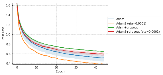 Figure 1
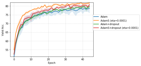 Figure 2
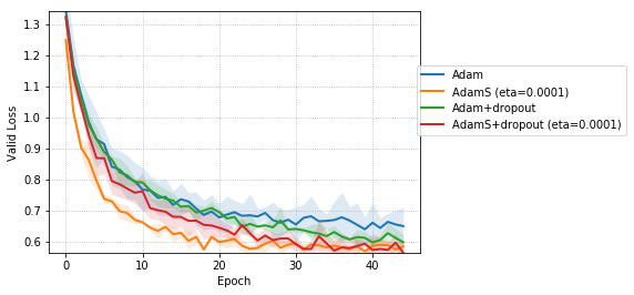 Figure 3
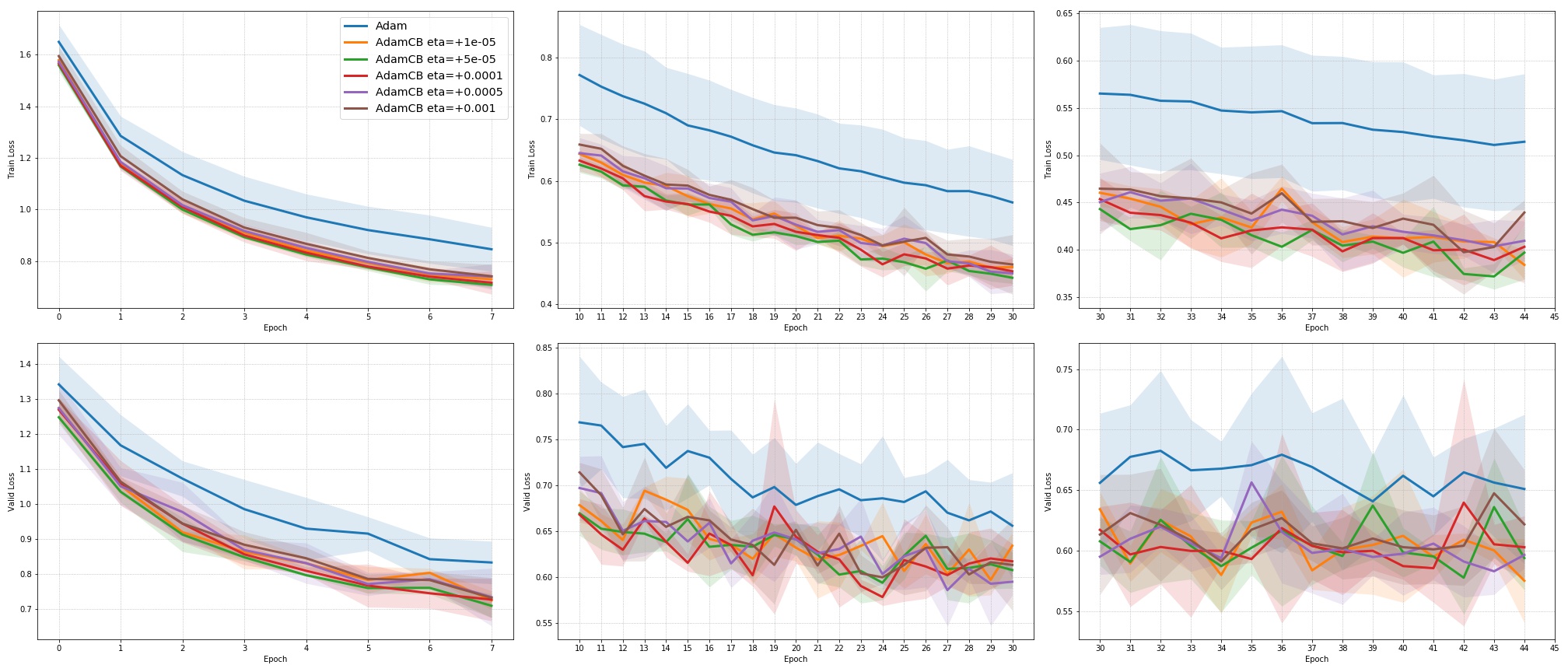 Figure 4
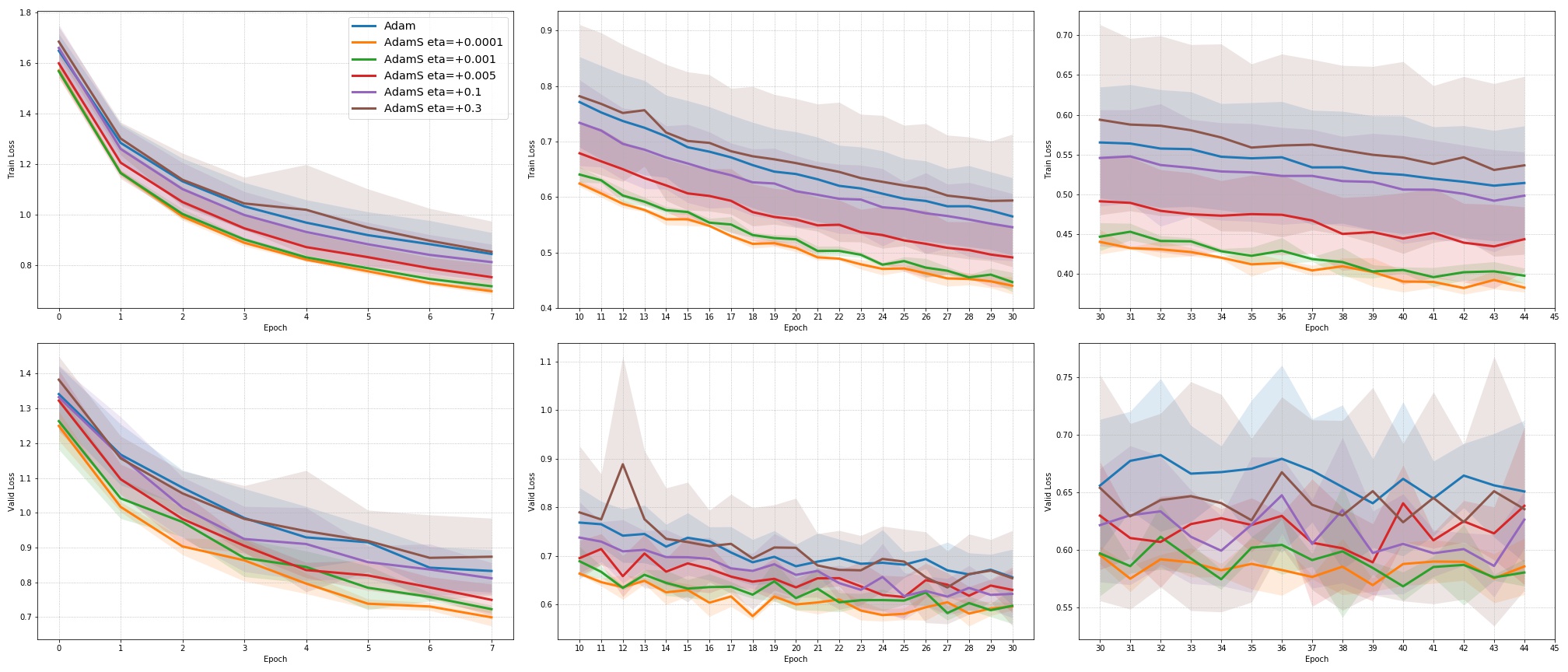 Figure 5
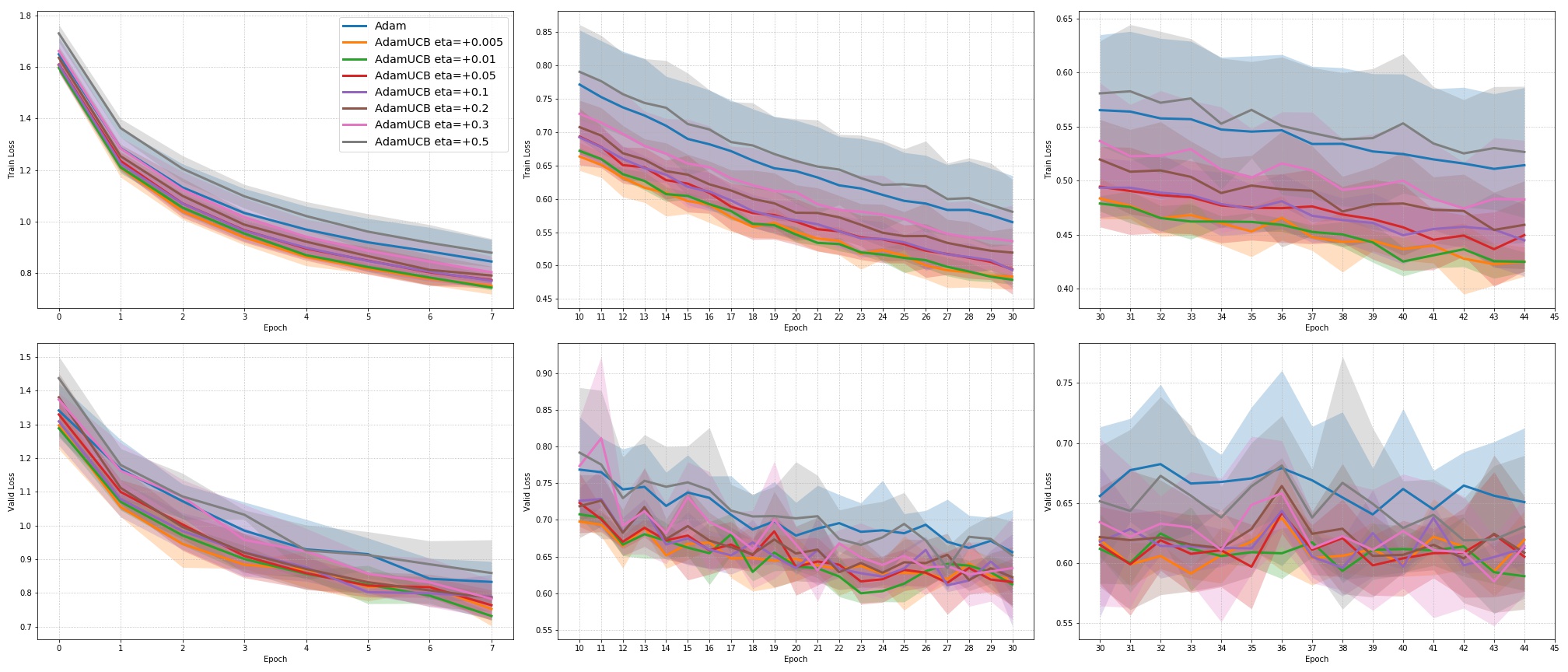 Figure 6
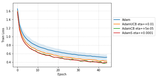 Figure 7
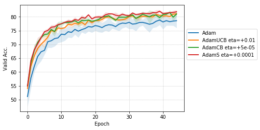 Figure 8
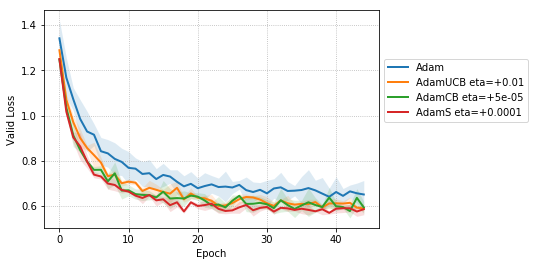 Figure 9
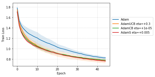 Figure 10
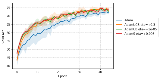 Figure 11
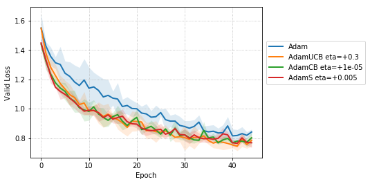 Figure 12
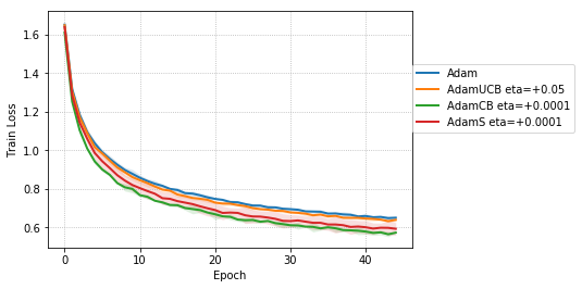 Figure 13
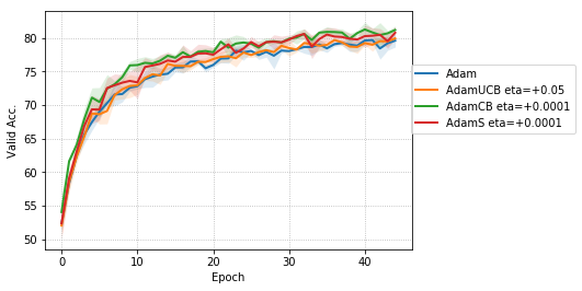 Figure 14
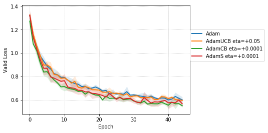 Figure 15
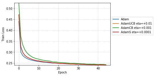 Figure 16
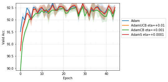 Figure 17
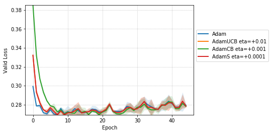 Figure 18
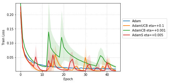 Figure 19
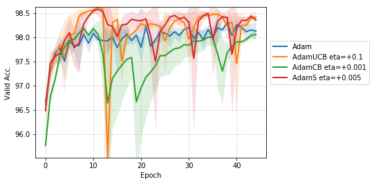 Figure 20
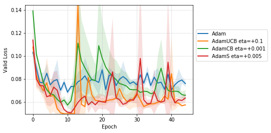 Figure 21
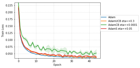 Figure 22
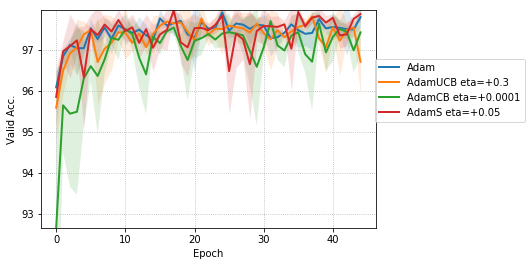 Figure 23
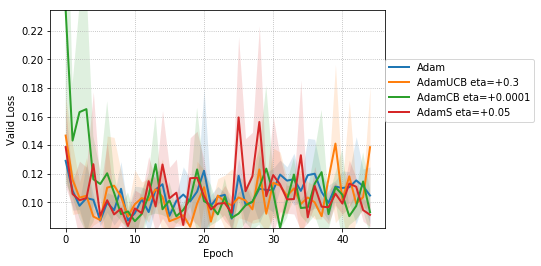 Figure 24
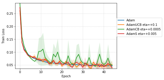 Figure 25
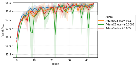 Figure 26
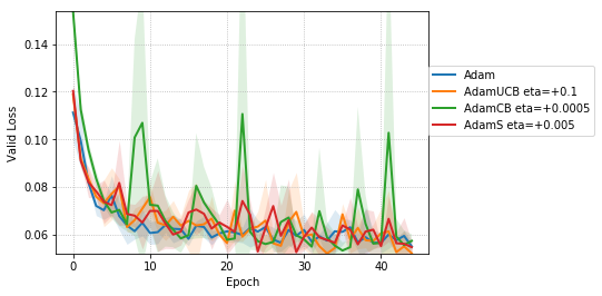 Figure 27
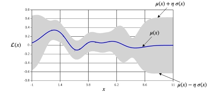 Figure 28
| Dataset | Model | Batch Size | Dropout | |||
| MNIST | LR | 128 | NO | |||
| MNIST | MLP | 128 | NO | |||
| YES | ||||||
| 16 | NO | |||||
| CIFAR-10 | CNN | 128 | NO | |||
| YES | ||||||
| 16 | NO |
| Epoch | Optimizer | Train Loss | Val. Loss | Val. Acc. (%) |
|---|---|---|---|---|
| 3 | Adam | |||
| AdamUCB | ||||
| AdamCB | ||||
| AdamS | ||||
| 20 | Adam | |||
| AdamUCB | ||||
| AdamCB | ||||
| AdamS | ||||
| 45 | Adam | |||
| AdamUCB | ||||
| AdamCB | ||||
| AdamS |
| Batch Size | Dropout | Epoch | Optimizer | Train Loss | Val. Loss | Val. Acc. (%) |
|---|---|---|---|---|---|---|
| 3 | Adam | |||||
| AdamUCB | ||||||
| AdamCB | ||||||
| AdamS | ||||||
| 20 | Adam | |||||
| NO | AdamUCB | |||||
| AdamCB | ||||||
| AdamS | ||||||
| 45 | Adam | |||||
| AdamUCB | ||||||
| AdamCB | ||||||
| 128 | AdamS | |||||
| 3 | Adam | |||||
| AdamUCB | ||||||
| AdamCB | ||||||
| AdamS | ||||||
| 20 | Adam | |||||
| YES | AdamUCB | |||||
| AdamCB | ||||||
| AdamS | ||||||
| 45 | Adam | |||||
| AdamUCB | ||||||
| AdamCB | ||||||
| AdamS | ||||||
| 3 | Adam | |||||
| AdamUCB | ||||||
| AdamCB | ||||||
| AdamS | ||||||
| 20 | Adam | |||||
| 16 | NO | AdamUCB | ||||
| AdamCB | ||||||
| AdamS | ||||||
| 45 | Adam | |||||
| AdamUCB | ||||||
| AdamCB | ||||||
| AdamS |
Peer Reviews
No public reviews on file for this paper yet. If you reviewed it on a platform where reviews are public (OpenReview, ICLR, NeurIPS, ICML), you can paste yours below so the community can read it here.
Code & Models
Videos
No videos yet. Explain this paper in a talk, walkthrough, or lecture? Add one.
Taxonomy
TopicsStochastic Gradient Optimization Techniques · Neural Networks and Applications · Advanced Neural Network Applications
MethodsAdam · REINFORCE
Exploiting Uncertainty of Loss Landscape for Stochastic Optimization
Vineeth S. Bhaskara
Department of Computer Science
University of Toronto
[email protected] Sneha Desai
Department of Computer Science
University of Toronto
Abstract
We introduce novel variants of momentum by incorporating the variance of the stochastic loss function. The variance characterizes the confidence or uncertainty of the local features of the averaged loss surface across the i.i.d. subsets of the training data defined by the mini-batches. We show two applications of the gradient of the variance of the loss function. First, as a bias to the conventional momentum update to encourage conformity of the local features of the loss function (e.g. local minima) across mini-batches to improve generalization and the cumulative training progress made per epoch. Second, as an alternative direction for "exploration" in the parameter space, especially, for non-convex objectives, that exploits both the optimistic and pessimistic views of the loss function in the face of uncertainty. We also introduce a novel data-driven stochastic regularization technique through the parameter update rule that is model-agnostic and compatible with arbitrary architectures. We further establish connections to probability distributions over loss functions and the REINFORCE policy gradient update with baseline in RL. Finally, we incorporate the new variants of momentum proposed into Adam, and empirically show that our methods improve the rate of convergence of training based on our experiments on the MNIST and CIFAR-10 datasets.
1 Introduction
††Code for our optimizers and experiments is publicly available at https://github.com/bsvineethiitg/adams.
Training deep neural networks by stochastic gradient descent has been highly successful in solving several important tasks in vision (He et al., 2016), language (Child et al., 2019), and Reinforcement Learning (RL) (Silver et al., 2017). Predominantly, the training procedure for modern deep neural networks involves some variation of vanilla stochastic gradient descent (SGD), where updates to the parameters are based on the gradient computed over the current mini-batch’s loss function.
The mini-batch gradient is a noisy unbiased estimator of the full-gradient. A widely used method to stabilize the mini-batch gradient is momentum, where parameter updates are based on an exponentially weighted average of the previous mini-batch gradients, thus "smoothing" out the oscillations in the updates (Goh, 2017). This improves training speed and convergence significantly (Sutskever et al., 2013), and has remained an essential component of modern optimization algorithms such as Adam and AdaMax (Kingma & Ba, 2014). In Section 3, we present an alternative perspective on why momentum (with the bias-correction term) works by showing that it approximates the full-gradient under certain assumptions and an exponential probability distribution.
In this paper, we propose exploiting the gradient of the second moment (or the "variance-gradient") of the stochastic loss function across mini-batches to quantify the uncertainty or error of the gradient of the first moment estimate (or the momentum) in approximating the full-gradient. The variance-gradient points along directions of the loss surface where the local features either conform or disagree the most across mini-batches.
In Section 4, we introduce MomentumUCB, a biased version of the momentum method that encourages updates along regions of the loss surface that locally conform across mini-batches in addition to the objective of minimizing the expected loss. In Section 5, we introduce MomentumCB and MomentumS that are biased and unbiased versions of the momentum, respectively, and exploit both the optimistic and pessimistic views of the loss surface in the face of uncertainty.
2 Related work
Previous work such as SAG (Roux et al., 2012), SAGA (Defazio et al., 2014) and SVRG (Johnson & Zhang, 2013) propose accelerating SGD through variance reduction of the mini-batch gradient by introducing a baseline for the gradient that is computed every steps.
Unlike the above work, our paper focuses on variance reduction of the underlying stochastic loss function rather than dealing directly with the variance of the gradient. Similar to SAG and SVRG, we introduce MomentumUCB, a biased estimator that has an additional variance minimization objective. We also empirically show that instead of maximizing or minimizing the variance of the stochastic loss objective throughout the optimization, exploration in the parameter space by alternating between optimistic and pessimistic views of the loss landscape accelerates training and provides an unbiased estimate of the full-gradient.
Similar to SAGA, we introduce MomentumS that is an unbiased estimator. In contrast to SAG, SAGA and SVRG, our variants of momentum introduced in the paper are computationally similar in cost to SGD with conventional momentum.
3 Momentum as an approximation to the full-gradient
Full-gradient
Consider the "full-loss" function under the parameters over the entire training dataset. Let the integer index denote mini-batch out of a total of mini-batches of the training dataset. Then one may write the full-batch loss function as \mathcal{L}({\boldsymbol{\theta}})=\mathbb{E}_{\mathcal{P}(i)}\bigg{[}\mathcal{L}^{(i)}({\boldsymbol{\theta}})\bigg{]} under . Therefore, the full-gradient at time step with parameters , may be explicitly written as:
[TABLE]
SGD with momentum and bias-correction term
Consider stochastic gradient descent with momentum and bias-correction term in Algorithm (1). At time step (with the current mini-batch labeled by ), one may unroll the recurrence for as
[TABLE]
Note that the operations on index are all done in modulo so that the indices still represent one of the mini-batches. In Algorithm (1), corresponds to an exponentially weighted sum (at timescale ) of the previous gradients across the mini-batches. The exponentially weighted average, , is obtained by dividing by the sum of the exponential weights , which precisely gives the term that is referred to as the "bias-correction term" in Adam (Kingma & Ba, 2014). Therefore, is the exponentially weighted average of the gradients across the mini-batches at time step . Writing explicitly, we have
[TABLE]
Compare Eq. (4) with the full-gradient in Eq. (1). Since one may not computationally afford to evaluate the network at the current parameters for each mini-batch to get the full-gradient at time step , momentum compromises to using an approximation for the full-gradient noting that when the learning rate is sufficiently small. An exponential decay weight proportional to is considered for the gradient at parameters as the approximation becomes less reasonable as gets larger. This can be noted by explicitly rewriting Eq. (4) as an expectation under an exponentially weighted probability distribution at a given time step (defined below) as follows:
[TABLE]
Thus, can be viewed as an approximation to the full-gradient at time step , mini-batch index mod, and parameters .
With this analogy in place, we approximate the gradient of the variance of the mini-batch loss function ("variance-gradient") under the exponentially weighted probability distribution defined above to derive an update rule similar to momentum.
4 MomentumUCB: Biasing momentum along low variance regions of the loss landscape
Consider the loss objective that accounts the variance of the loss function to bias the updates along the regions of the landscape that conform across the mini-batches up to an extent determined by the "confidence hyperparameter" as follows:
[TABLE]
where the subscript corresponds to a probability distribution over the mini-batches and . The above loss objective is similar in form to the Upper Confidence Bound (UCB) acquisition function in Bayesian optimization that is maximized to balance exploration with exploitation.
The additional variance-minimization objective encourages generalization by providing an incentive for performing equally well on individual i.i.d. subsets of the training data (defined by the mini-batches) separately to keep the variance of the loss lower.
Figure (1) illustrates the resultant optimization landscape in 1D, as an example, for the cases of (pessimism) and (optimism) in the face of uncertainty.
Considering the gradient of in Eq. (6), one has:
[TABLE]
where \sigma_{l}^{2}=\text{Var}_{i}[\mathcal{L}^{(i)}({\boldsymbol{\theta}})]=\mathbb{E}_{i}\left[\left(\mathcal{L}^{(i)}({\boldsymbol{\theta}})\right)^{2}\right]-\left(\mathbb{E}_{i}\big{[}\mathcal{L}^{(i)}({\boldsymbol{\theta}})\big{]}\right)^{2}, and \mu_{l}=\mathbb{E}_{i}\bigg{[}\mathcal{L}^{(i)}({\boldsymbol{\theta}})\bigg{]}.
We infer the update rule for computing by approximating the expectation in Eq. (9) under the exponentially weighted probability distribution . We refer to the resultant update rule as MomentumUCB to distinguish it from the conventional momentum update.
AdamUCB: Adam with MomentumUCB
Considering the stochastic gradient at time step to be , one may write the traditional Adam update concisely as , where s are the time scales, and denotes under the exponentially decaying probability distribution.
We introduce AdamUCB in Algorithm (2) that implements MomentumUCB (Eq. (9)) in the parameter update rule as follows
[TABLE]
where is the mini-batch loss at the current time step , {} are the mean and the standard deviation of mini-batch losses up to time step , respectively, and is the confidence hyperparameter.
4.1 Connections to policy gradient with baseline in reinforcement learning
Consider a typical setting of a RL problem with representing the cumulative reward for a roll out . The goal is to maximize the expected return, , where represents the probability of the roll out that depends both on the policy and the dynamics of the environment.
The REINFORCE policy gradient update with baseline can be written as . A common choice for the baseline is the average return obtained so far, i.e., . Substituting into REINFORCE, we have
[TABLE]
Consider the MomentumUCB gradient from Eq. (9) as follows:
[TABLE]
Simplifying the variance-gradient term, we have
[TABLE]
Therefore, when and in Eq. (13) are chosen to be the negative cross-entropy loss in a supervised learning setting, for instance, and the co-variance is instead computed across the mini-batches, then the policy gradient term in Eq. (13) reduces to the variance-gradient in Eq. (15).
5 Exploiting pessimism and optimism in the face of uncertainty
In the previous section, we introduced MomentumUCB justifying the case for as taking a pessimistic view of the loss surface that biases updates along regions that conform across mini-batches. An undesirable effect of such a variance-minimization objective is that the parameters might eventually land on a plateau of the loss surface, preventing further progress and slowing down training. In this section we propose incorporating the best of both the cases of (pessimism in the face of uncertainty) and (optimism in the face of uncertainty) where the updates alternate between maximizing and minimizing the variance objective based on a criterion.
5.1 Bounding the relative standard deviation by on both sides
We propose a simple modification to the MomentumUCB term in Eq. (9) by replacing with the difference of the current relative standard deviation (defined by ) and the required relative standard deviation (specified by a hyperparameter that is different from the in MomentumUCB) that must be maintained throughout the optimization. The intuition behind this criterion is that the variance of the loss landscape should not be too low (to avoid undesirable plateaus of the surface) or too high (since a "good" minima likely performs comparably well across the i.i.d. mini-batches).
Replacing , we have the following version of Momentum that we call MomentumCB or Confidence bounded Momentum since the standard deviation is bounded on both the sides (two-sided bound):
[TABLE]
When the current relative std. dev. is greater than the specified hyperparameter , the term takes a positive sign (with a magnitude proportional to the violation) and updates along directions that reduce the variance (in addition to the usual momentum gradient), and, hence, takes a pessimistic view of the loss surface. Similarly, when the current relative std. dev. is lower than the hyperparameter , the updates get biased along directions that increase the variance.
AdamCB: Adam with MomentumCB
We incorporate MomentumCB into Adam under the exponential probability distribution (similar to Algorithm (2)). The parameter update rule for AdamCB is given by
[TABLE]
5.2 The reparametrization trick and stochastic momentum
In this section we introduce a stochastic regularizer based on the variance-gradient that utilizes both the directions of minimizing and maximizing the variance to randomly "explore" in the parameter space.
By "exploration," especially, in the context of non-convex optimization, we refer to choosing a perturbed parameter based on the variance-gradient after a conventional momentum update step. This acts as an initialization for the subsequent update and allows access to multiple regions of the loss surface over the course of training. Also, unlike dropout (Srivastava et al., 2014), our stochastic regularizer is architecture and model agnostic, and, therefore, is compatible with batch normalization (Li et al., 2018).
If in the Eq. (6) is promoted to a new random variable such that , where is a Gaussian distribution and specifies the variance of the Gaussian (different from in MomentumUCB), then we have the loss function also promoted to a random variable in such that
[TABLE]
Therefore, instead of fixing in MomentumUCB, if one samples it from a Gaussian distribution centered around zero with a specified standard deviation (given by a new hyperparameter ), then one can exploit both the directions of minimizing and maximizing the variance during the optimization.
By the reparametrization trick (Kingma & Welling, 2013), sampling in the above equation for is equivalent to sampling a loss function from a Gaussian distribution over mini-batch loss functions, i.e.,
[TABLE]
before computing the gradient. We call the approximation of under the exponential probability distribution as Stochastic Momentum or MomentumS since is a stochastic variable in .
Interestingly, since is a random variable in , its expectation over the Gaussian results in an unbiased estimate of the full-gradient. That is,
[TABLE]
since when . Therefore, MomentumS is an unbiased estimate of the full-gradient when is sampled from at each step.
With recent high-capacity deep neural networks such as OpenAI Five (OpenAI, 2018) being trained for several months continuously, "exploration" in the parameter space ensures that the optimization is not wastefully stuck on a plateau or bounded within a local region.
AdamS: Adam with Stochastic Momentum
We incorporate Stochastic Momentum into Adam by sampling in AdamUCB (see Algorithm (2)) from a zero-centered Gaussian whose standard deviation is provided as a hyperparameter.
6 Experiments
We empirically evaluate the three variants of Adam, namely, AdamUCB, AdamCB and AdamS and compare their performance with the original Adam optimizer. We train multiple architectures of neural networks such as logistic regression (see Figure 2), MLPs (see Figure 3), CNNs (see Figure 4) on MNIST/CIFAR-10 datasets on a single nVIDIA Tesla P4 GPU. The architectures of the networks are chosen to closely resemble the experiments published by Kingma & Ba (2014).
Since our comparison is only among Adam-like optimizers, we use a fixed learning rate of (without any scheduling) and do not search over different s. This is because the RMSprop-like denominator in all of our proposed variants ensures the step size to be roughly the same as Adam. We also use a weight-decay of , batch size of 128, and keep the values of and fixed to Adam defaults of 0.9 and 0.999, respectively, across all our experiments. The input images are pre-processed by normalizing with the mean and the standard deviation of the pixel values. Best hyperparameter obtained by searching over a grid is used for each variant of the optimizer in the comparison. We present detailed results for additional training configurations (such as different batch sizes, etc) in the appendices.
7 Discussion
For the simple case of logistic regression on MNIST, the original Adam algorithm performs the best across the training metrics (Figure 2). Since convex objectives have an unique solution, the advantage of "exploration" along variance-gradient direction diminishes.
From Figure 3, for the case of MLPs trained on MNIST, AdamS and AdamUCB achieve a lower training and validation loss on average than Adam. For instance, at epoch 20 and 45, AdamS achieves half and one-third of the training error of Adam, respectively.
For CNNs trained on CIFAR-10 (Figure 4), AdamUCB, AdamCB and AdamS perform significantly better the original Adam optimizer when no dropout is used ( 6% improvement in val. acc. at epoch = 3). Not only is the validation loss better for our variants of Adam but also is the rate of convergence of training. We notice that AdamCB and AdamS consistently perform better than AdamUCB in this case. This shows that exploiting both the directions of variance-gradient indeed helps. For the case of CNNs with dropout, AdamCB and AdamS still outperform Adam but with a reduced margin of improvement ( 2% improvement in val. acc. at epoch = 3).
Figure 5 compares the effect of adding dropout to Adam and AdamS for the case of CNNs trained on CIFAR-10 dataset. The stochastic regularization implemented by AdamS leads to faster training convergence and better validation error when compared to dropout regularization.
8 Conclusion and future work
In this paper, we introduced novel ways of incorporating the variance information of the loss landscape across mini-batches for stochastic optimization. Based on our experiments with CIFAR-10, we recommend AdamS for optimizing general non-convex objectives (a good default for is ).
Our work opens up directions of incorporating existing research on exploration–exploitation trade-off in Bayesian optimization into gradient-based stochastic optimization algorithms. Interesting directions for future research include exploiting other acquisition functions like Probability of Improvement (PI), Expected Improvement (EI), among others, to design loss objectives that efficiently utilize the uncertainty information of the loss landscape to accelerate training.
Investigating SGD with variations of momentum proposed in this paper could also prove to be interesting as our formulation naturally gives a schedule for the learning rate through the variance of the loss. Finally, analyzing the effect of decay schedules for , AdaMax-like modifications to the proposed variants of Adam, and incorporating Nesterov’s momentum-like update rule (Nesterov, 1983; Dozat, 2016) would be other interesting directions to pursue.
Contributions
V.S.B. contributed to the theory, derivations, and the experiments on CIFAR-10 dataset using CNN architectures. S.D. verified the derivations and contributed to the experiments on MNIST using Logistic Regression and MLPs.
Acknowledgments
We greatly acknowledge the supervision of our project by Prof. Jimmy Ba and Prof. Roger Grosse at the University of Toronto. We also acknowledge the Vector Institute Scholarship in Artificial Intelligence (VSAI) for supporting our graduate studies towards MSc in Applied Computing (MScAC).
Appendix A Additional details on our experiments and results
We report the mean and the standard deviation for various performance metrics such as loss and accuracy across three random runs of our experiments. The hyperparameter is tuned for each variant of the optimizer, and the best values found are listed in Table 1.
A.1 Experiment: Logistic Regression
Table 2 summarizes the training and validation scores at different stages of the training under the four optimizers (Adam, AdamUCB, AdamCB and AdamS) for the best values of given in Table 1.
A.2 Experiment: Multi-layer Neural Networks
We additionally experiment by adding a dropout noise layer () over the output activations of the first hidden layer, and study the effect of different batch sizes.
Table 3 and Figure 6 summarize the training, and validation performances for batch sizes 16 and 128 for the best values of given in Table 1 at different stages of the training.
A.3 Experiment: Convolutional Neural Networks
We include results of our experiments with batch size = 16. Figure 7 shows the improvement in the rate of convergence for the case of batch size = 16. Figure 8 summarizes the results of our experiments without dropout on a mini-batch size of across different . Table 4 summarize the training, and validation performances for batch sizes 16 and 128 for the best values of given in Table 1 at different stages of the training.
Appendix B Discussion
For the case of MLPs with dropout, AdamS outperforms Adam but with a reduced margin of improvement (see Table 3) when compared to the case without dropout. When a batch size of 16 is used instead, AdamS and Adam perform fairly similar.
For the case of CNNs trained on CIFAR-10, clearly, from the Figure 8, AdamUCB, AdamCB and AdamS perform significantly better for appropriate s than the original Adam optimizer. Figure 7 shows how the proposed versions of Adam accelerate training for batch size = 16. We also notice that the improvement in performance for lower mini-batch sizes is more significant for CIFAR-10.
Table 4 clearly shows how our variants of Adam accelerate training, especially, in the initial few epochs for CIFAR-10 dataset for both the cases of mini-batch sizes 16 and 128. When dropout is used, the improvement in validation accuracy reduces by some margin. ∎
The reference list from the paper itself. Each links out to its DOI / PubMed record.
- 1Child et al. (2019) Rewon Child, Scott Gray, Alec Radford, and Ilya Sutskever. Generating long sequences with sparse transformers. ar Xiv e-prints , art. ar Xiv:1904.10509, Apr 2019.
- 2Defazio et al. (2014) Aaron Defazio, Francis Bach, and Simon Lacoste-Julien. Saga: A fast incremental gradient method with support for non-strongly convex composite objectives. In Advances in Neural Information Processing Systems , pp. 1646–1654, 2014.
- 3Dozat (2016) Timothy Dozat. Incorporating nesterov momentum into adam. 2016.
- 4Goh (2017) Gabriel Goh. Why momentum really works. Distill , 2(4):e 6, 2017.
- 5He et al. (2016) Kaiming He, Xiangyu Zhang, Shaoqing Ren, and Jian Sun. Deep residual learning for image recognition. In Proceedings of the IEEE Conference on Computer Vision and Pattern Recognition , pp. 770–778, 2016.
- 6Johnson & Zhang (2013) Rie Johnson and Tong Zhang. Accelerating stochastic gradient descent using predictive variance reduction. In Advances in Neural Information Processing Systems , pp. 315–323, 2013.
- 7Kingma & Ba (2014) Diederik P Kingma and Jimmy Ba. Adam: A method for stochastic optimization. ar Xiv preprint ar Xiv:1412.6980 , 2014.
- 8Kingma & Welling (2013) Diederik P Kingma and Max Welling. Auto-encoding variational bayes. ar Xiv preprint ar Xiv:1312.6114 , 2013.