Cross-section measurements of radiative proton-capture reactions in $^{112}$Cd at energies of astrophysical interest
A. Psaltis, A. Khaliel, E.-M. Assimakopoulou, A. Kanellakopoulos, V., Lagaki, M. Lykiardopoulou, E. Malami, P. Tsavalas, A. Zyriliou, T. J., Mertzimekis
TL;DR
This study measures the cross sections of the $^{112}$Cd(p,$ extgamma$)$^{113}$In reaction at astrophysically relevant energies, providing new experimental data to inform nucleosynthesis models and compare with theoretical predictions.
Contribution
First experimental determination of the $^{112}$Cd(p,$ extgamma$)$^{113}$In cross sections within the Gamow window using two complementary techniques.
Findings
Cross sections measured at astrophysical energies.
Astrophysical S factors and isomeric ratios deduced.
Results compared with Hauser-Feshbach calculations.
Abstract
Reactions involving the group of nuclei commonly known as p nuclei are part of the nucleosynthetic mechanisms at astrophysical sites. The In nucleus is such a case with several open questions regarding its origin at extreme stellar environments. In this work, the experimental study of the cross sections of the radiative proton-capture reaction Cd(p,)In is attempted for the first time at energies lying inside the Gamow window with an isotopically enriched Cd target. Two different techniques, the in-beam -ray spectroscopy and the activation method, have been applied. The latter method is required to account for the presence of a low-lying In isomer at 392 keV having a halflife of min. From the cross sections, the astrophysical S factors and the isomeric ratios have been additionally deduced. The experimental results are…
Click any figure to enlarge with its caption.
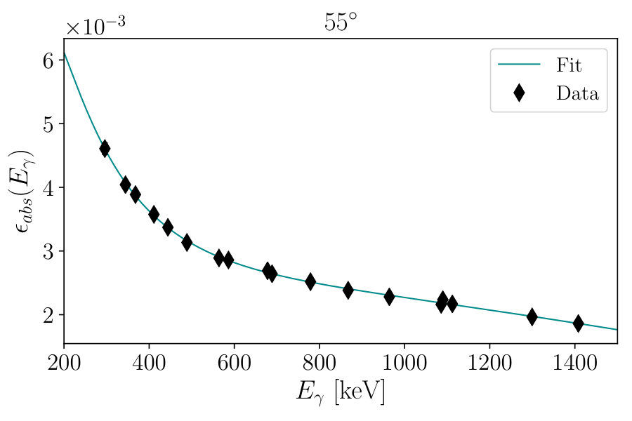 Figure 1
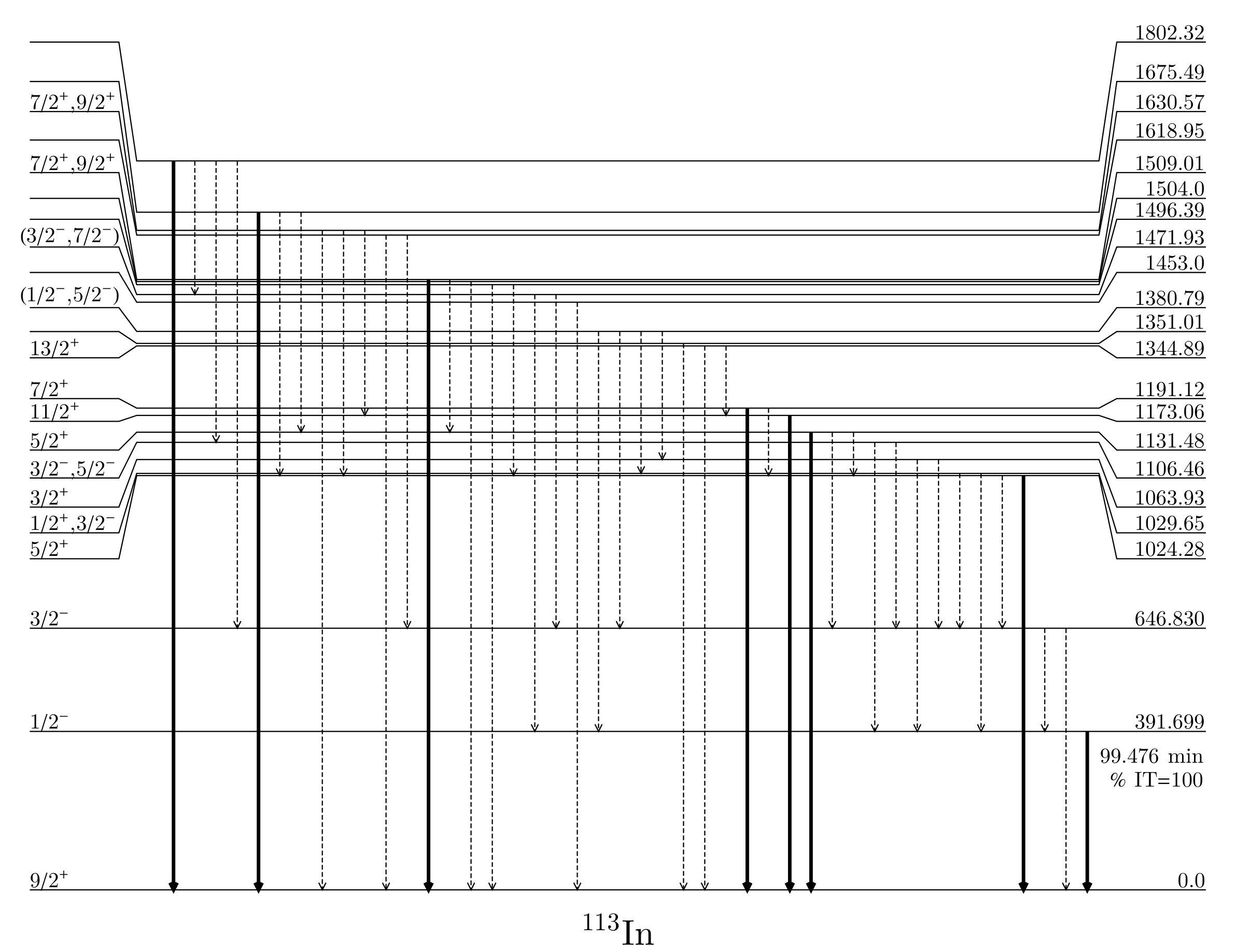 Figure 2
 Figure 3
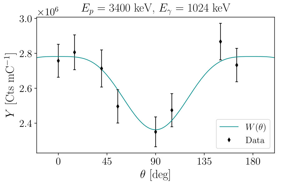 Figure 4
 Figure 5
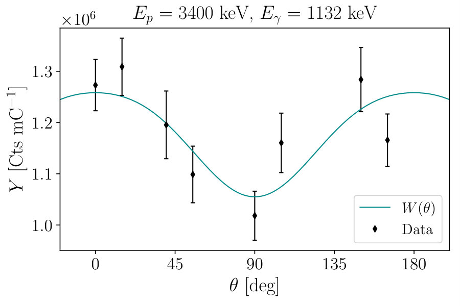 Figure 6
 Figure 7
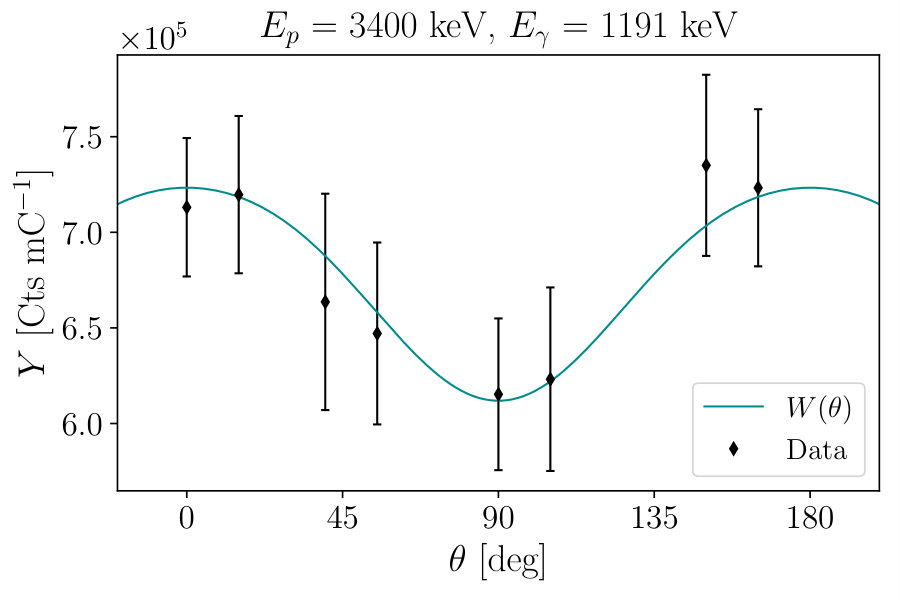 Figure 8
 Figure 9
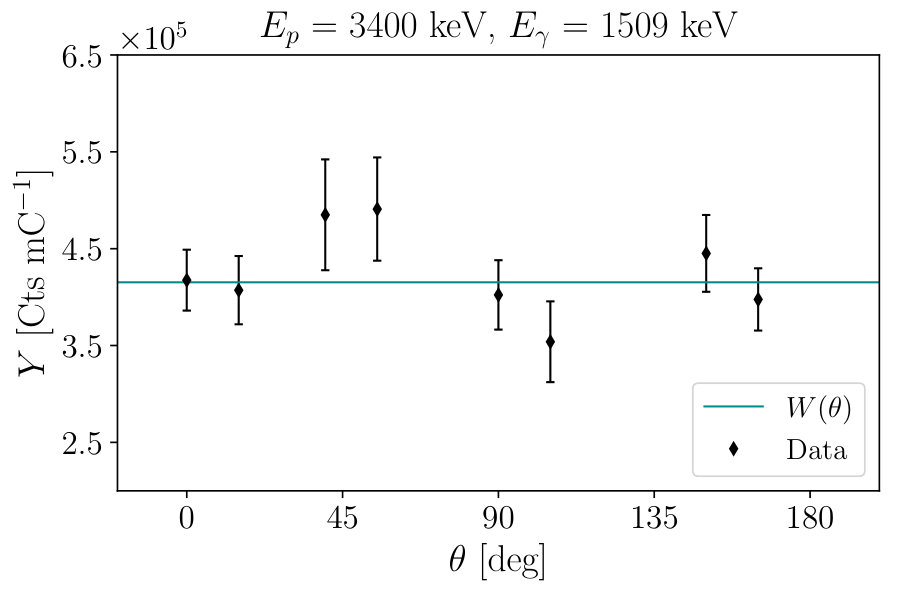 Figure 10
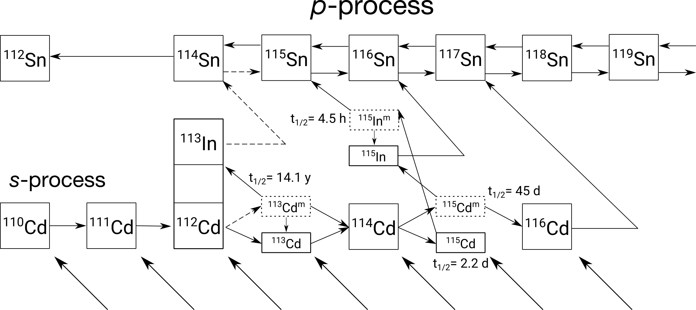 Figure 11
 Figure 12
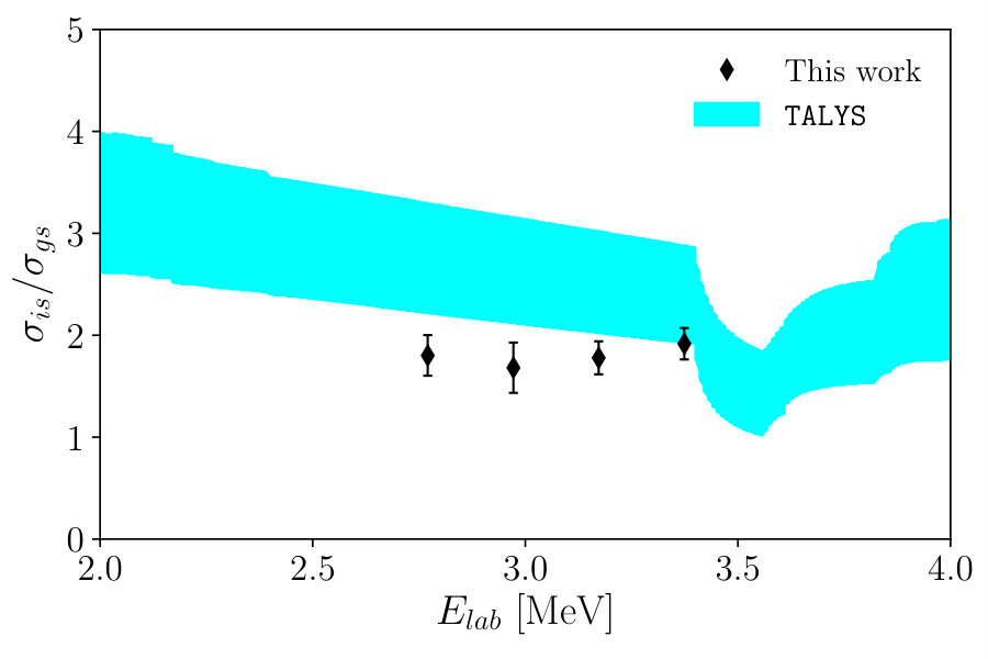 Figure 13
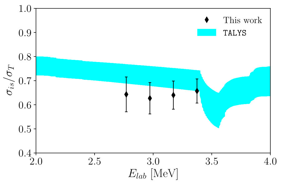 Figure 14
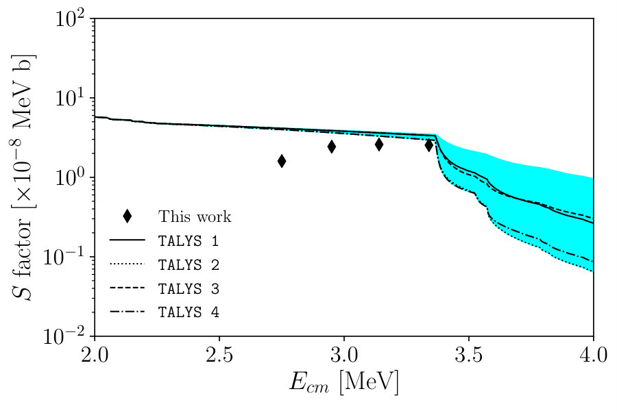 Figure 15
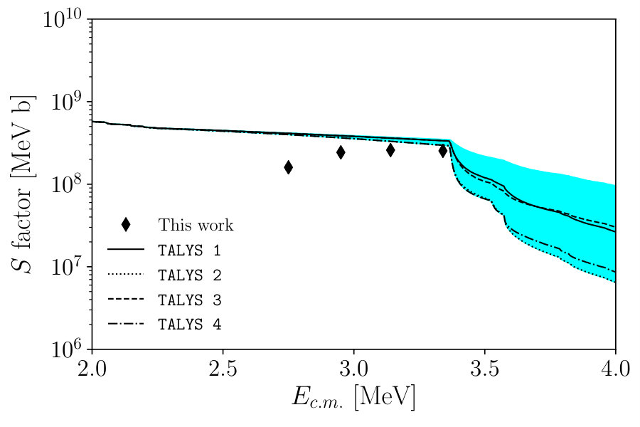 Figure 16
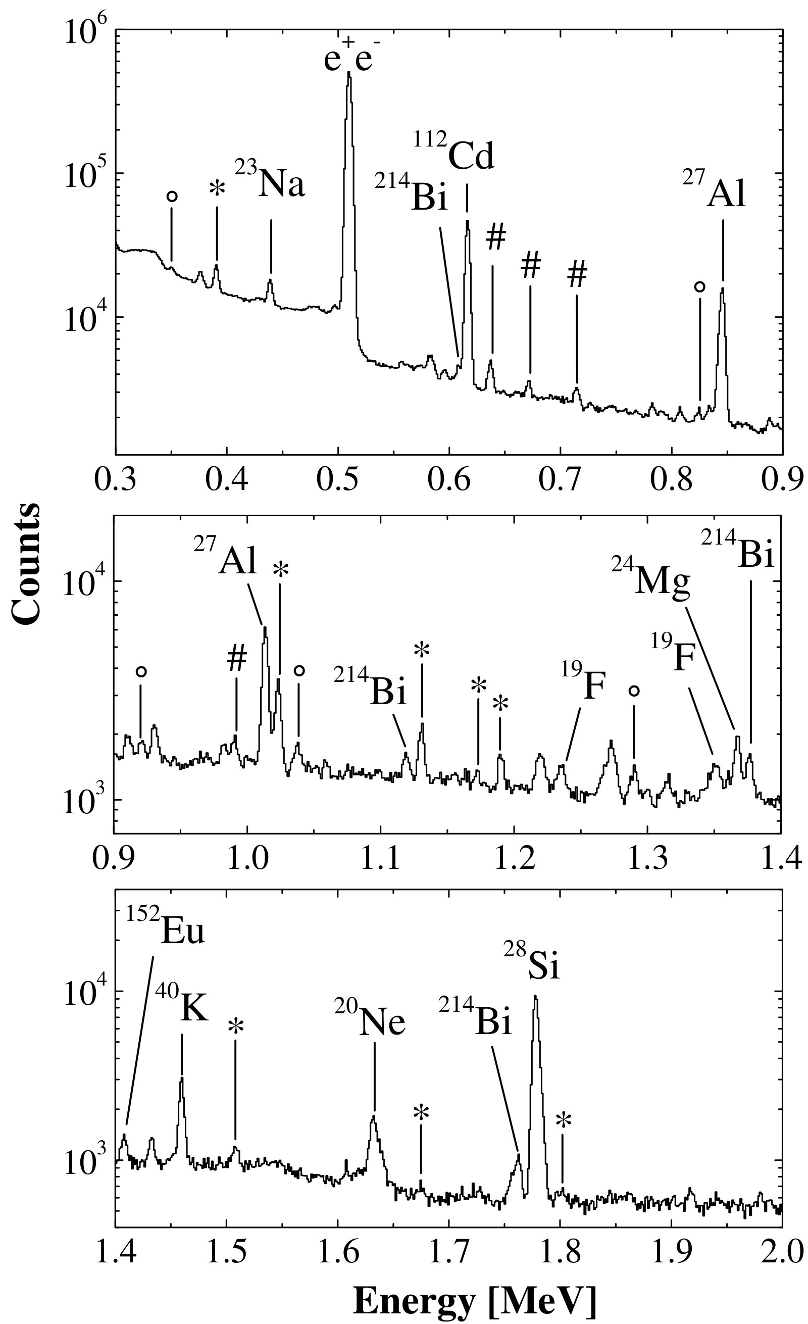 Figure 17
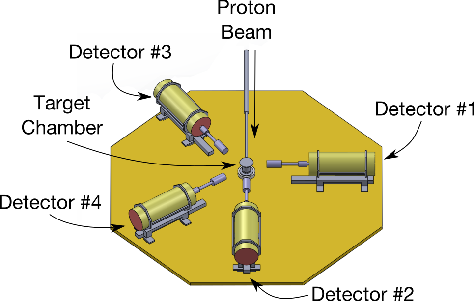 Figure 18
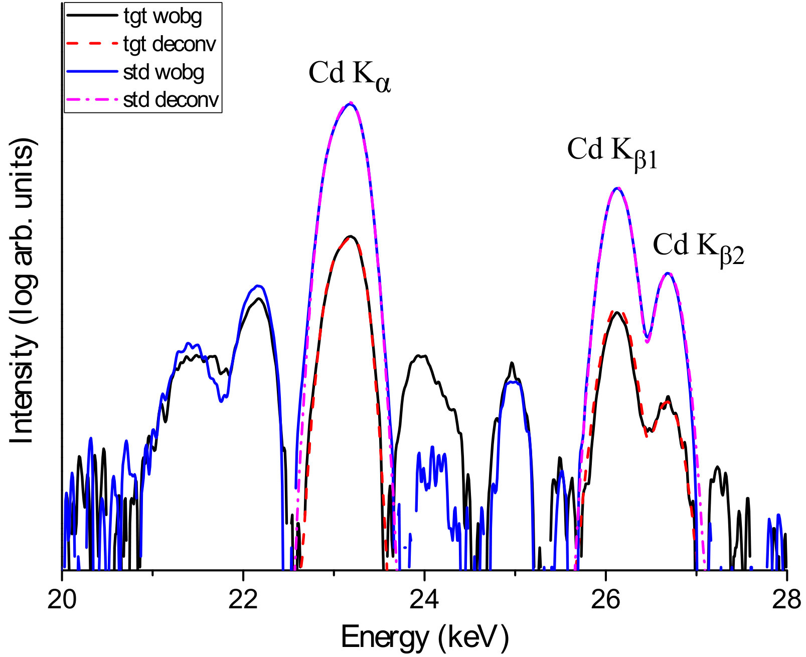 Figure 19
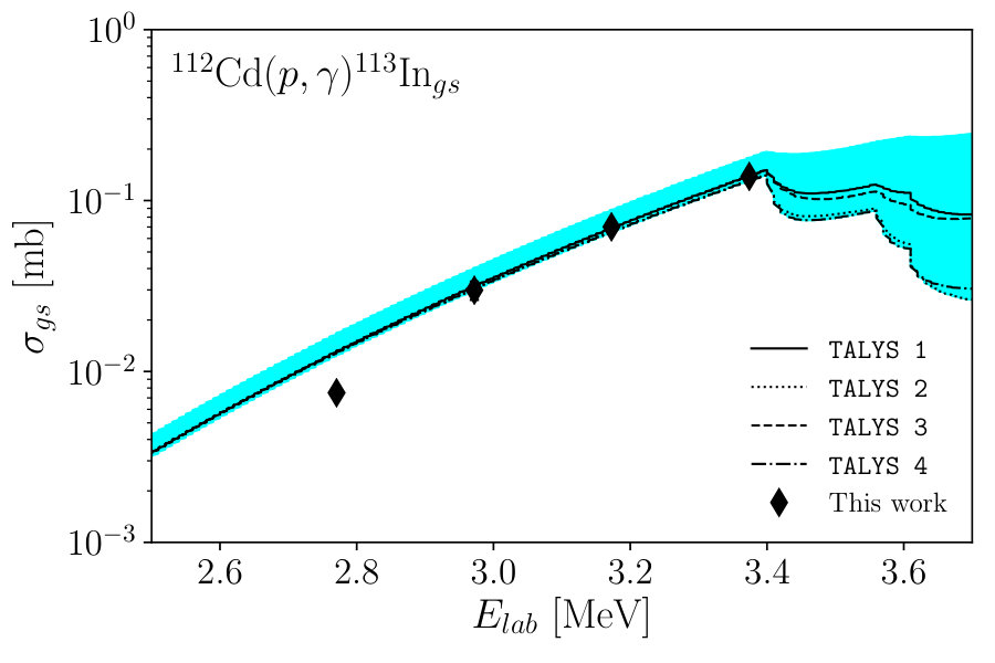 Figure 20
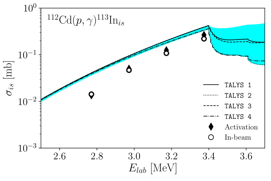 Figure 21
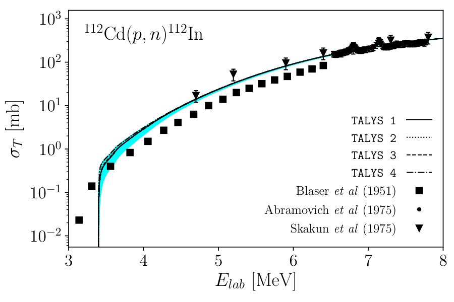 Figure 22
 Figure 23
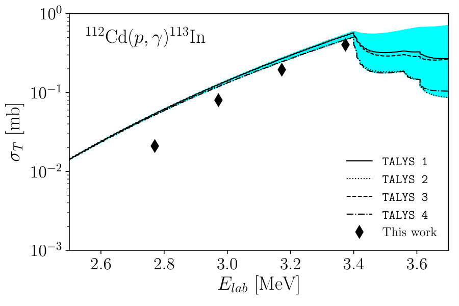 Figure 24
| E keV | |
| E keV | |
| E keV | |
| E keV | |
| E keV | |
| unknown | E keV |
| unknown | E keV |
| (lab) | (lab) | (c.m.) | S factor | |||||
|---|---|---|---|---|---|---|---|---|
| (MeV) | (MeV) | (MeV) | (mb) | (mb) | (mb) | ( MeV b) | ||
| 2.800 | 2.771 | 2.746 | ||||||
| 3.000 | 2.972 | 2.945 | ||||||
| 3.200 | 3.172 | 3.144 | ||||||
| 3.400 | 3.374 | 3.344 |
| Optical Model Potential | Nuclear Level Density | Strength Function |
|---|---|---|
| Koning–Delaroche (KD) Koning and Delaroche (2003) | Constant Temperature Model (CTM) Gilbert and Cameron (1965) | Kopecky–Uhl Kopecky and Uhl (1990) |
| Bauge–Delaroche–Girod (BDG) Bauge et al. (2001) | Back–shifted Fermi gas model (BSFG) Dilg et al. (1973) | Brink–Axel Brink (1957); Axel (1962) |
| Generalized Superfluid Model (GSM) Ignatyuk et al. (1993) | Hartree–Fock BCS (HFBCS) Capote et al. (2009) | |
| Goriely Tables Goriely et al. (2001) | Hartree–Fock–Bogolubov (HFB) Capote et al. (2009) | |
| Hilaire Tables Goriely et al. (2008) | Goriely Hybrid Model Goriely (1998) | |
| T–dependent HFB, Gogny force (TDHFB) Hilaire et al. (2012) | Goriely TDHFB Hilaire et al. (2012) | |
| T–Dependent RMF Arteaga and Ring (2008) | ||
| Gogny D1M HFB+QRPA Martini et al. (2014) |
| (lab) | (Activation) | (In–beam) | Deviation |
|---|---|---|---|
| (MeV) | (mb) | (mb) | (%) |
| 2.771 | 0.014 0.001 | 0.0143 0.0008 | 2 |
| 2.972 | 0.050 0.004 | 0.047 0.004 | 6 |
| 3.172 | 0.125 0.009 | 0.108 0.006 | 14 |
| 3.374 | 0.265 0.016 | 0.220 0.011 | 17 |
Peer Reviews
No public reviews on file for this paper yet. If you reviewed it on a platform where reviews are public (OpenReview, ICLR, NeurIPS, ICML), you can paste yours below so the community can read it here.
Videos
No videos yet. Explain this paper in a talk, walkthrough, or lecture? Add one.
Present address: ] Department of Physics and Astronomy, McMaster University, Hamilton, ON L8S 4M1, Canada
Present address: ] Department of Physics and Astronomy, Uppsala, Sweden
Present address: ] Instituut voor Kern– en Stralingsfysica, KU Leuven, Celestijnenlaan 200D, B–3001 Leuven, Belgium
Present address: ] CERN, Geneva, Switzerland
Present address: ] Department of Physics and Astronomy, University of British Columbia, 6224 Agricultural Road, Vancouver, BC V6T1Z1, Canada
Present address: ] Nikhef, Science Park 105, 1098 XG, Amsterdam, Netherlands
Cross–section measurements of radiative proton–capture reactions
in \isotope[112]Cd at energies of astrophysical interest
A. Psaltis
[
Department of Physics, National Kapodistrian University of Athens, Zografou Campus, GR–15784, Athens, Greece
A. Khaliel
Department of Physics, National Kapodistrian University of Athens, Zografou Campus, GR–15784, Athens, Greece
E.–M. Assimakopoulou
[
Department of Physics, National Kapodistrian University of Athens, Zografou Campus, GR–15784, Athens, Greece
A. Kanellakopoulos
[
Department of Physics, National Kapodistrian University of Athens, Zografou Campus, GR–15784, Athens, Greece
V. Lagaki
[
Department of Physics, National Kapodistrian University of Athens, Zografou Campus, GR–15784, Athens, Greece
M. Lykiardopoulou
[
Department of Physics, National Kapodistrian University of Athens, Zografou Campus, GR–15784, Athens, Greece
E. Malami
[
Department of Physics, National Kapodistrian University of Athens, Zografou Campus, GR–15784, Athens, Greece
P. Tsavalas
Department of Physics, National Kapodistrian University of Athens, Zografou Campus, GR–15784, Athens, Greece
INRASTES, NCSR “Demokritos”, GR–15310, Aghia Paraskevi, Greece
A. Zyriliou
Department of Physics, National Kapodistrian University of Athens, Zografou Campus, GR–15784, Athens, Greece
T.J. Mertzimekis
Corresponding author: [email protected]
Department of Physics, National Kapodistrian University of Athens, Zografou Campus, GR–15784, Athens, Greece
Abstract
Reactions involving the group of nuclei commonly known as p nuclei are part of the nucleosynthetic mechanisms at astrophysical sites. The \isotope[113]In nucleus is such a case with several open questions regarding its origin at extreme stellar environments. In this work, the experimental study of the cross sections of the radiative proton–capture reaction \isotope[112]Cd()\isotope[113]In is attempted for the first time at energies lying inside the Gamow window with an isotopically enriched \isotope[112]Cd target. Two different techniques, the in–beam –ray spectroscopy and the activation method, have been applied. The latter method is required to account for the presence of a low–lying \isotope[113]In isomer at 392 keV having a halflife of min. From the cross sections, the astrophysical S factors and the isomeric ratios have been additionally deduced. The experimental results are compared to detailed Hauser–Feshbach theoretical calculations using TALYS, and discussed in terms of their significance to the optical model potential involved.
p nuclei, \isotope[112]Cd, \isotope[113]In, cross section, Hauser–Feshbach theory
pacs:
24.60.Dr, 25.40.Lw, 27.60.+j
††preprint: APS/123-QED
I Introduction
The origin of some 35 neutron–deficient stable isotopes with mass , between \isotope[74]Se and \isotope[196]Hg, in the neutron–deficient side of the valley of stability, commonly known as “p nuclei”, has been one of the major open questions in nuclear astrophysics Burbidge et al. (1957); Cameron (1957). The solar abundances of p nuclei are one to two orders of magnitude lower compared to the respective r and s nuclides in the same mass region Lodders et al. (2009), which is attributed to “shielding” by their reaction flow Arnould and Goriely (2003); Rauscher et al. (2013).
Various astrophysical environments and associated processes have been proposed to explain the origin of the p nuclei and their solar abundances. The main mechanism is referred to as the p process, but it is used interchangeably with the term process, which also plays a dominant role to this nucleosynthesis scenario Woosley and Howard (1978). The p process is assumed to occur in different zones inside a core–collapse supernovae, and thus the peak temperature for the p process lies between GK Arnould and Goriely (2003). It has also been shown that the p process can also occur in a single–degenerate type Ia supernovae scenario Travaglio et al. (2011).
Several other explosive nucleosynthesis scenarios, such as the rp process Schatz et al. (1999), the pn process Goriely et al. (2002) and the p process Fröhlich et al. (2006); Pruet et al. (2006); Wanajo (2006) have been proposed to contribute to the production of p nuclei. It is remarkable that despite the variety of astrophysical models, these processes can reproduce the solar abundances of the p nuclei within a factor of 3 (e.g. see the sensitivity study by Rapp et al. Rapp et al. (2006)). Nevertheless, several species, such as \isotope[92,94]Mo, \isotope[96,98]Ru, \isotope[113]In and \isotope[115]Sn, are significantly underproduced in most models. In the context of the present work, the origin of \isotope[113]In is discussed in some detail later in the text.
The vast p process reaction network involves roughly reactions among nuclei Arnould and Goriely (2003) and thus, within that framework, most of the reaction rates need to be estimated using the Hauser–Feshbach statistical model Hauser and Feshbach (1952).
The experimental input is invaluable in terms of constraining the model parameters. Measurements of cross sections in radiative proton–capture reactions can play a two–fold pivotal role towards the understanding of the p process. First, they can be used to adjust the parameters of the statistical model improving theoretical predictions for currently unmeasured reactions, and second, they can make calculations of important photodisintegration decay constants possible José and Iliadis (2011).
Open questions on the origin of \isotope[113]In
The production of \isotope[113]In at astrophysical sites has been a long–standing puzzle for nuclear astrophysics Ward and Beer (1981). \isotope[113][]In is the lightest in a group of four p nuclei that are not even–even111The other three are \isotope[115]Sn, \isotope[138]La and \isotope[180m]Tam. \isotope[138]La is considered to be produced by the process ( flows from core–collapse supernovae) Woosley et al. (1990). Rauscher et al. (2013), and has a relatively high elemental contribution of 4.3% Lodders et al. (2009).
The complexity of nucleosynthesis in the Cd–In–Sn region arises mainly due to the existence of several long–lived –decaying isomers Németh et al. (1994); Theis et al. (1998) (see also Fig. 1) and leads to significant underproduction of the rare odd–A isotopes \isotope[113]In and \isotope[115]Sn Rapp et al. (2006).
Nemeth et al. Németh et al. (1994) proposed a s–process contribution to the origin of \isotope[113]In, which was calculated to be very small (less than 1%). Recent calculations, using KADoNiS Dillmann et al. (2006) have resulted in a much smaller, 0.0013% contribution.
Theis et al. have showed that post–r process –decay chains could account for less than 12% of the solar abundance of \isotope[113]In, and that thermally enhanced decay of the progenitor \isotope[114]Cd is possible Theis et al. (1998). Finally, Dillmann et al. Dillmann et al. (2007, 2008) proposed the –delayed r process decay chains as the most promising scenario.
The rp and p processes are excluded as possible production mechanisms, since they generally produce nuclei up to Dillmann et al. (2008). In this context, a p process sensitivity study by Wanajo et al. Wanajo et al. (2011) has demonstrated that by changing either astrophysical or nuclear physics input parameters, the p process could account for the origin of \isotope[113]In and other p nuclei.
Concerning possible astrophysical sites, Fujimoto et al. showed in Ref. Fujimoto et al. (2007) that \isotope[113]In and several other underproduced p nuclei can be abundantly synthesized in ejecta originated by a collapsar Woosley (1993). Specifically, the heavy p nuclei, including \isotope[113]In, are produced in the jets through fission Fujimoto et al. (2007).
Interestingly enough, it has been demonstrated by Babishov and Kopytin Babishov and Kopytin (2006); Kopytin and Hussain (2013) that \isotope[113]In could be produced during a supernova explosion of a star. However, their final p abundances are accompanied by underestimated molybdenum and ruthenium abundances, still leaving some open questions.
As a consequence of all the above, it is nowadays widely accepted that \isotope[113]In is not a “pure” p nucleus, but has non–negligible contributions from the s and r processes Pignatari et al. (2016).
Many studies have focused on \isotope[113]In in the vicinity of –process nucleosynthesis energies, such as the \isotope[113,115]In()\isotope[114,116]Sn reactions Harissopulos et al. (2016), the elastic scattering Kiss et al. (2013), and the \isotope[113]In()\isotope[117]Sb reactions Yalçın et al. (2009). Recently, Muhammed Shan et al. Shan et al. (2018) focused on proton–induced reactions in \isotope[113]In at energies ranging 8–22 MeV adding information to earlier investigations of the \isotope[112]Cd()\isotope[113]In reaction Blaser et al. (1951); Abramovich et al. (1975); Skakun et al. (1975). The spin isomer in \isotope[113]In was also very recently studied in the pygmy resonance region with photoexcitation Nedorezov et al. (2019).
In the present work, we report on a first experimental attempt to study the radiative proton capture relevant to the production of \isotope[113]In by measuring the reaction cross sections at astrophysically interesting energies, using an isotopically enriched \isotope[112]Cd target. Despite the particular reaction is not necessarily a strong channel in the reaction flow Rauscher (2006), it can still be considered valuable to have its cross section measured, as it can assist in constraining models to offer better predictions for reactions that can not be measured directly in this mass regime.
II Experimental Details
Measurements for the study of the radiative proton capture reaction on \isotope[112]Cd were carried out at the 5.5 MV T11 Tandem Van de Graaff accelerator of the NCSR “Demokritos” in Athens, Greece. Both the in–beam and activation methods have been used in the measurements to account for a low–lying isomeric state in the populated nucleus \isotope[113]In.
II.1 The Proton Beams
The reaction \isotope[112]Cd()\isotope[113]In ( keV) qva was studied at four proton lab energies in total, i.e. 2.8, 3.0, 3.2 and 3.4 MeV. All energies lie inside the Gamow Window for temperatures related to the production of p nuclei with at GK, which corresponds to MeV. During the experiments the target was irradiated with protons of beam currents ranging enA.
II.2 The Target
A multi–layer target was irradiated during the experiments, comprising a front layer of 99.7% enriched \isotope[112]Cd evaporated on a \isotope[nat]Bi layer, backed by an \isotope[nat]In layer and a thick \isotope[nat]Cu layer. Considering the generally low proton–capture cross section at these energies and the low natural abundance of \isotope[112]Cd, the use of an enriched target was imperative. The thick \isotope[nat]Cu backing provided efficient charge collection during the experiment.
The \isotope[112]Cd layer thickness was measured equal to mg/cm2 with the Rutherford Backscattering Technique (RBS) before and after the experiment and found to have no degradation due to irradiation Gyürky, Gy. et al. (2019). To further confirm the layer thickness, an independent measurement was carried out after the experiment using X–ray Fluorescence Spectroscopy (XRF) resulting in a value of mg/cm2. The two results were combined to produce the average value of mg/cm2, where the error cited is the standard deviation calculated from the two measurements.
The target was turned inside the chamber by with respect to the beam to avoid having its aluminum frame masking any of the surrounding HPGe detectors, in particular the one sitting at 90∘ (see also Ref. Khaliel et al. (2017)), thus resulting in an effective thickness of the target, mgcm*-2*.
Proton–beam energy losses in the target were calculated using SRIM2013 Ziegler et al. (2010) and found to be keV for the corresponding proton beam energies MeV in the laboratory frame. Assuming reactions taking place in the middle of the \isotope[112]Cd layer, the effective energy in the center–of–mass system is given by (see also Table 1):
[TABLE]
A voltage of V was applied to the target chamber to suppress the emission of secondary electrons from altering the charge collection readings, which are essential for the calculation of the reaction yields and subsequently the cross section. The target was mounted on an aluminum heatsink cooled externally by an air–pumping system.
II.3 Detection Apparatus & Experimental Methods
An array of four high–purity Germanium (HPGe) detectors of 100% relative efficiency was mounted on an octagonal turntable with maximum radius 2.4 m (Fig. 3). The table’s turning ability enables measurements of a full angular distribution. This particular setup is known of its versatility on measuring cross sections and angular distributions of radiative capture reactions relevant to the p process. Similar studies can be found in Refs. Galanopoulos et al. (2003); Sauerwein et al. (2012); Khaliel et al. (2017).
Detectors 1–4 were initially placed at 90, 0, 55 and 165 degrees, respectively, with reference to the beam direction. Their distances from the target were 15.5, 15.5, 14.8 and 18.0 cm, respectively. By turning the table by 15 degrees counterclockwise, an additional set of angles was used (105, 15, 40, 150 degrees respectively). Energy calibrations and absolute efficiency measurements (Fig. 5) for all detectors were performed with a standard \isotope[152]Eu point source placed in the exact target position, before and after the experiments. Spectra were recorded in singles mode using the nuclear electronics setup described in Ref. Khaliel et al. (2017).
Due to the structure properties of \isotope[113]In (see level scheme in Fig. 4), two different methods were employed to study the cross–section of the radiative proton capture reaction: in–beam –ray spectroscopy, and activation.
A low–lying isomeric state of \isotope[113]In (=391.7 keV, min (see Ref. nnd for the data and Fig. 4 for a partial level scheme) was populated in the reactions. Due to the particular lifetime of the state, a measurement of the corresponding cross section relies on the exploitation of the activation method. In the recent past, similar studies have successfully employed the activation technique Yalçin et al. (2009); Kiss et al. (2011); Dillmann et al. (2011); Sauerwein et al. (2011); Halász et al. (2012); Netterdon et al. (2013, 2014); Güray et al. (2015); Kinoshita et al. (2016). For a more detailed description concerning the application of the activation method on proton–induced reactions relevant to the p process, the reader is referred to Refs. Gyürky et al. (2003); Gyürky, Gy. et al. (2019).
In the present case, the activation method was combined efficiently with the in–beam measurements. The duration of irradiation was kept at 6–8 h, to ensure that the isomeric state has been populated sufficiently and (almost) reached saturation. Following irradiation, overnight measurements for over five half–lives ( min) were performed, without beam delivery on the target. Activation measurements followed in–beam measurements for each proton beam energy used in this study.
III Data Analysis and Results
III.1 In–beam measurements
The cross section of the reaction \isotope[112]Cd()\isotope[113]Ings can be estimated from the relation Rolfs and Rodney (1988):
[TABLE]
where is the atomic mass of the target in a.m.u., is the Avogadro number, is the actual target thickness in and is the absolute yield of the reaction in counts per . The latter can be deduced from:
[TABLE]
where the coefficients are related to the angular distributions of the emitted photons originating from the –th transition feeding the ground state of the residual nucleus:
[TABLE]
where the are coefficients which depend on the spin and parity of the initial and final state of the transition, and are Legendre polynomials. From the level scheme of the residual nucleus \isotope[113]In (Fig. 4), seven transitions feeding the ground state were observed with statistics above the background:
Typical examples of measured angular distributions are shown in Fig. 7, showing the –transition angular pattern for the transitions , , , and at beam energy of keV. In cases where an angular distribution was not clearly demonstrated in the data (mainly due to large uncertainties), an average value was used instead (see e.g. lower right panel in Fig. 7). In addition, no was observed in the spectra, likely due to the large spin difference between the entry state (1/2+ or 3/2+) and the ground state of \isotope[113]In (Jπ=9/2+). The results for the ground state cross section are tabulated in Table 1 and plotted in Fig. 8.
III.2 Activation measurements
The isomeric transition is characterized by a half life of min. The measurement of the absolute yield of the particular transition demanded the use of the activation method. An additional measurement of the cross section of the isomeric state was performed with the in–beam method that was discussed in the previous paragraph.
For each beam energy, the target was irradiated for approximately three half–lives, which is a sufficient irradiation time interval, as after about , the process reaches saturation Iliadis (2015). The isomeric cross section was evaluated using the standard relation:
[TABLE]
where is the number of events under the corresponding photopeak of the isomeric transition, is the probability of –ray emission, is the decay constant of the transition, is the number of target nuclei per unit area, is the incident proton flux during the irradiation, is the absolute efficiency of the detector and , , are the waiting (or cooling) time of the sample, the counting time and the irradiation time of the sample, respectively. For the present case, and s*-1* end ; Blachot (2010).
The results for the isomeric cross sections with the activation method are tabulated in Table 1 and plotted in Fig. 9 (solid diamonds). Errors were evaluated by considering the uncertainties from photopeak integration, the detector efficiencies and the charge deposition on the target during the irradiation of the sample. Cross–section results for the isomeric state deduced from the in–beam technique taking into account all transitions reaching the isomeric state are shown in the same figure (empty circles).
III.3 Total cross–sections and astrophysical S factors
The total cross section of the reaction 112Cd()113In, , have been evaluated by adding the cross sections of all transitions feeding the ground state of the produced nucleus (summing to the in–beam cross section ) and the cross–section of the isomeric state, , as measured with the activation technique described earlier:
[TABLE]
The results for the total cross section of the studied reaction are tabulated in Table 1 and plotted in Fig. 10. After measuring the total cross section, the astrophysical S factor can be deduced, by means of the relation:
[TABLE]
where is the Sommerfeld parameter Yakovlev et al. (2010). The results for the astrophysical S factor are also tabulated in Table 1 and plotted in Fig. 12. The particular quantity is important for astrophysical applications, as it varies smoothly with energy, compared to the cross section, thus allowing for safer extrapolations to experimentally inaccessible energies, serving also as a useful quantity for reaction network calculations.
All energies selected for the experiment reside inside the Gamow window and below the reaction threshold at energy of MeV qva (see Table 1 for details).
III.4 Hauser–Feshbach calculations with TALYS
Theoretical calculations using the Hauser–Feshbach statistical model have been performed with the TALYS v1.9 code Koning et al. (2007). A total of 96 different combinations of the main ingredients of the model, i.e. the Optical Potential (OMP) (2 default options), the Nuclear Level Density (NLD) (6 default options) and the –ray Strength Function (SF) (8 default options) have been used. The models used are presented in Table 2. The calculations were performed using a 5–keV energy step, between 1.5 and 8.0 MeV using the supercomputing facility Z–machine at NCSR “Demokritos”.
Both microscopic and phenomenological models have been used for calculations, using the default parameters provided by TALYS. For the OMP, the phenomenological model of Koning–Delaroche Koning and Delaroche (2003), as well as the semi–microscopic model of Bauge–Delaroche–Girod Bauge et al. (2001) has been used. It is important to note that, at the studied energy range, which lies below the Coulomb barrier, the OMP, and in particular its imaginary component, is known to depend strongly on the energy Arnould and Goriely (2003).
All six available NLD models provided by TALYS have been used in the calculations, namely the phenomenological Constant–Temperature model (CTM) Gilbert and Cameron (1965), the Back–shifted Fermi gas model Dilg et al. (1973), the Generalized Superfluid model Ignatyuk et al. (1993), the semi–microscopic level density tables of Goriely Goriely et al. (2001), and Hilaire Goriely et al. (2008), and values using the Time–Dependent Hartree–Fock–Bogolyubov method combined with the Gogny force Hilaire et al. (2012).
Regarding SF models, the Kopecky–Uhl Kopecky and Uhl (1990) and Brink–Axel Brink (1957) generalized lorentzians were used, as well as values calculated using the Hartree–Fock–BCS and Hartree–Fock–Bogolyubov methods Capote et al. (2009). Goriely’s hybrid model Goriely (1998), as well as Goriely’s tables using the temperature–dependent Hartree–Fock–Bogolyubov method were additionally employed. Last, models using the Temperature–Dependent Relativistic Mean Field method Hilaire et al. (2012) and the Hartree–Fock–Bogolyubov method along with the Quasi–Random–Phase–Approximation using the Gogny D1M interaction Martini et al. (2014) have been considered.
After performing all possible calculations with the models described above, the maximum and minimum for each energy has been determined, defining the borders of the light blue area shown in Figs. 8–12. The calculations (TALYS 1–4) that best describe the ground–state cross section, based on direct comparison with the experimental data, have been also included in the plots: TALYS 1 and TALYS 2 employ the Koning–Delaroche OMP, while TALYS 3 and TALYS 4 use the Bauge–Delaroche–Girod OMP; TALYS 1 and TALYS 3 employ the Generalized Superfluid model NLD and the HFBCS SF, while TALYS 2 and TALYS 4 use the TDHFB with the Gogny force NLD model and the Temperature–dependent RMF SF model.
IV Discussion and Conclusions
In the framework of the present work, an experimental attempt to measure the total reaction cross section and the S factor of the astrophysically important reaction \isotope[112]Cd()\isotope[113]In has been carried out for the first time. The cross section was measured inside the astrophysically relevant energy range, at four beam energies, namely 2.8, 3.0, 3.2 and 3.4 MeV.
The measurement of the total reaction cross section required the use of two different techniques. The cross section of all prompt transitions feeding the ground state of the produced nucleus was determined using the in–beam –angular distribution method. All visible transitions in the spectra feeding the isomeric state were included in the measurement of its cross section. However, due to the significantly longer half–life of the isomeric state the activation technique was employed Rolfs and Rodney (1988); Gyürky, Gy. et al. (2019) additionally and was used to produce the total cross section. Table 3 lists the two data sets for each energy value and the % deviation of the cross section deduced from the in–beam method from the corresponding value found with the activation technique.
The absolute yields of seven (7) transitions feeding directly the ground state of \isotope[113]In have been measured. It has to be stressed that the cross sections are particularly small (7.5–138 b for the in–beam measurements; 14–265 b for the activation measurements) posing a real difficulty in collecting sufficient statistics, especially for the low–populated states decaying directly to the ground state at the lowest energy of 2.8 MeV. A few of the corresponding transitions hide under the background built up in singles mode, thus resulting in some missing yield. However, in the present work, this missing yield can be safely considered smaller than the experimental error for the two lower energies (Fig. 9).
An alternative experimental approach to remedy all that could possibly be the application of the detection method, which simplifies the tedious data analysis of a complex –ray spectrum, since it results into a single summing peak. The aforementioned method has been applied successfully for studies in reactions relevant to the p process Spyrou et al. (2007) despite its own constraints, such as the summing efficiency, which depends on the –decay scheme Iliadis (2015).
As mentioned earlier, the cross section of the isomeric state was measured using the activation technique in addition to measuring transitions feeding the isomeric state during the application of the in–beam technique. Compared to the latter case, in the activation method, there is no beam–induced background in the spectra and no angular distribution effect to consider. In the present case, the decay of the \isotope[113]In isomer emits 392–keV rays, where the efficiencies of the detectors are relatively better, compared with the higher–energy transitions measured with the in–beam method. However, it is of extreme importance to have accurate knowledge of the half–life and the branching ratios of the isomeric state, as the measurement explicitly depends on their values (see Eq. 5).
Combining the ground–state cross sections from the in–beam technique and the isomeric cross sections from the activation technique (see data listed in Table 1) the total cross sections, , for the reaction \isotope[112]Cd()\isotope[113]In has been deduced for all four energy values, ranging 21–404 b (also in Table 1). These results show a smooth increase with increasing energy as illustrated in Fig. 10. The values were used further to calculate the astrophysical S factors by means of Eq. 7, also included in Table 1. The S factor values exhibit an almost constant behavior, except for the lower energy point at beam energy 2.8 MeV, as it is evident from the data trend in Fig. 12.
From the experimental data in Table 1, the isomeric–to–ground state cross section ratio, , and the isomeric–to–total cross section ratio, , can be evaluated, as well. The isomeric cross section ratios are particularly useful in understanding the transfer of angular momentum in nuclear reactions. The results are shown in the two far–right columns in the same Table and shown in Fig. 13. Both ratios remain almost constant at different energies. Their weighted–averages have been deduced: and .
Theoretical calculations using the Hauser–Feshbach model have been performed, incorporating all possible combinations of the default TALYS parameters of the models tabulated in Table 2. The range of all calculations for each energy for the total cross section is plotted in Fig. 10, along with the experimental data. As expected, below the energy threshold of the () channel ( keV), the dependence from the NLD and SF models is relatively weak. In this energy range, the cross section depends almost exclusively on the choice of the OMP parameters, as it is evident in the convergence of all calculations at low energies.
Despite some overestimation, the theoretical predictions describe the trend of the experimental data fairly well (Figs. 8–10). TALYS 1–4 calculations agree well with the in–beam results with some small overestimation at 2.8 MeV for the ground state (Fig. 8). For the isomeric state, the theoretical trend is in fair agreement with the experimental results except the lowest energy point (Fig. 9), despite an overall overestimation of the cross section data, which is subsequently reflected on the total cross section (Fig. 10). There is no obvious reason for this minor disagreement from an experimental point of view. To further investigate the situation, the employed TALYS models have to be revisited more carefully, especially in regards of the OMP involved. Such disagreements have been observed in other cases in this mass regime (see e.g. Gyürky et al. (2001), the review article by Gyürky et al. Gyürky, Gy. et al. (2019) and references therein) and require careful consideration of the statistical uncertainties included in the models, as well as more detailed experimental work.
Along these lines, the () channel can offer some useful insights. Calculations for the cross sections of the () channel have been performed simultaneously with the () channel. These calculations are compared with existing experimental data, as shown in Fig. 11. The theoretical results seem to agree well with the data above 6.0 MeV, but theoretical calculations seem to diverge from the data below that energy value down to the () energy threshold. Also, two different sets of experimental data, those by Blaser et al. Blaser et al. (1951) and Skakun et al. Skakun et al. (1975), seem to significantly disagree with one another in the energy range between 4.5 and 6.2 MeV, and both with the present calculation (more the former, less the latter). However, the combinations TALYS 1–4, which best describe the ground–state cross section of the () channel, seem to also describe the data of Skakun et al. rather well.
It could be argued that the observed disagreement between the data and the theoretical calculations is due to the fact that the incorporated phenomenological and semi–microscopic OMPs have been optimized at significantly higher energy range than the one the present study focuses on. Consequently, an extrapolation to energies lower than the () threshold may be responsible for the overestimation of the experimentally deduced total reaction cross section data. However, it has to be noted that a full sensitivity analysis of the OMP parameters is beyond the scope of this work, as this would require careful consideration of all models involved in the calculation, scrutinizing the respective statistical uncertainties, and potentially fine–tuning the numerous model parameters.
Overall, the present work provides the first set of experimentally deduced cross sections, astrophysical S factors and isomeric ratios in \isotope[113]In populated in a proton–capture radiative reaction. The new information can support the improvement of reaction network calculations around the p nucleus . Certainly, further investigation is required in this region of the nuclear chart, both theoretically and experimentally, to provide firm insight at the driving mechanisms behind the p process reaction network, as well as to improve the phenomenological parts of the Optical Model Potentials in an energy region where a scarcity of experimental data, even for stable nuclei, still persists.
Acknowledgements.
The authors gratefully acknowledge the technical and scientific staff of the Tandem Accelerator Laboratory at NCSR “Demokritos” for their support during the experiment and useful discussions. We thank E. Mavrommatis for useful discussions, C. Markou and K. Pikounis for assistance in using the supercomputing facility at NCSR “D” and Dr. K. Mergia for providing access to the XRF spectroscopy station. A. Khaliel acknowledges support from the Hellenic Foundation for Research and Innovation (HFRI) and the General Secretariat for Research and Technology (GSRT), under the PhD Fellowship grant (GA. no. 74117/2017), and is thankful to the organizers, lecturers and fellow trainees of the ChETEC training school “An experiment of Nuclear Physics for Astrophysics using direct methods”, hosted by IFIN-HH of Bucharest-Magurele, for the fruitful discussions on the activation method. P. Tsavalas has performed work within the framework of the EUROfusion Consortium which has received funding from the Euratom research and training programme 2014-2018 and 2019-2020 under grant agreement No 633053. The views and opinions expressed herein do not necessarily reflect those of the European Commission. We are grateful to an anonymous reviewer for providing constructive comments resulting in an overall improvement of the present work.
The reference list from the paper itself. Each links out to its DOI / PubMed record.
- 1Burbidge et al. (1957) E. M. Burbidge, G. R. Burbidge, W. A. Fowler, and F. Hoyle, Rev. Mod. Phys. 29 , 547 (1957).
- 2Cameron (1957) A. G. W. Cameron, Publ. Astron. Soc. Pac. 69 , 201 (1957).
- 3Lodders et al. (2009) K. Lodders, H. Palme, and H.-P. Gail, in Solar system (Springer, 2009), pp. 712–770.
- 4Arnould and Goriely (2003) M. Arnould and S. Goriely, Phys. Rep. 384 , 1 (2003).
- 5Rauscher et al. (2013) T. Rauscher, N. Dauphas, I. Dillmann, C. Fröhlich, Z. Fülöp, and G. Gyürky, Rep. Prog. Phys. 76 , 066201 (2013).
- 6Woosley and Howard (1978) S. Woosley and W. Howard, Astrophys. J. Suppl. Ser. 36 , 285 (1978).
- 7Travaglio et al. (2011) C. Travaglio, F. K. Röpke, R. Gallino, and W. Hillebrandt, Astrophys. J. 739 , 93 (2011).
- 8Schatz et al. (1999) H. Schatz, L. Bildsten, A. Cumming, and M. Wiescher, Astrophys. J. 524 , 1014 (1999).