Composite Higgs at high transverse momentum
Andrea Banfi, Barry M. Dillon, Wissarut Ketaiam, and Sandra, Kvedarait\.e

TL;DR
This paper investigates how light top-partners in composite Higgs models influence Higgs+Jet production at the LHC, especially at high transverse momentum, revealing dependence on top-partner representations.
Contribution
It analyzes the effects of light top-partners on Higgs production and transverse momentum spectra, highlighting the role of top-partner representations in composite Higgs scenarios.
Findings
Corrections to Higgs couplings depend on top-partner representations.
Light top-partners significantly affect the Higgs transverse momentum spectrum.
Associated production can probe new physics scales not accessible via gluon fusion.
Abstract
In this paper we explore composite Higgs scenarios through the effects of light top-partners in Higgs+Jet production at the LHC. The pseudo-Goldstone boson nature of the Higgs field means that single-Higgs production via gluon fusion is insensitive to the mass spectrum of the top-partners. However in associated production this is not the case, and new physics scales may be probed. In the course of the work we consider scenarios with both one and two light top-partner multiplets in the spectrum of composite states. We study corrections to the Higgs couplings and the effects that the light top-partner multiplets have on the transverse momentum spectrum of the Higgs. Interestingly, we find that the corrections to the Standard Model expectation depend strongly on the representation of the top-partners in the global symmetry.
Click any figure to enlarge with its caption.
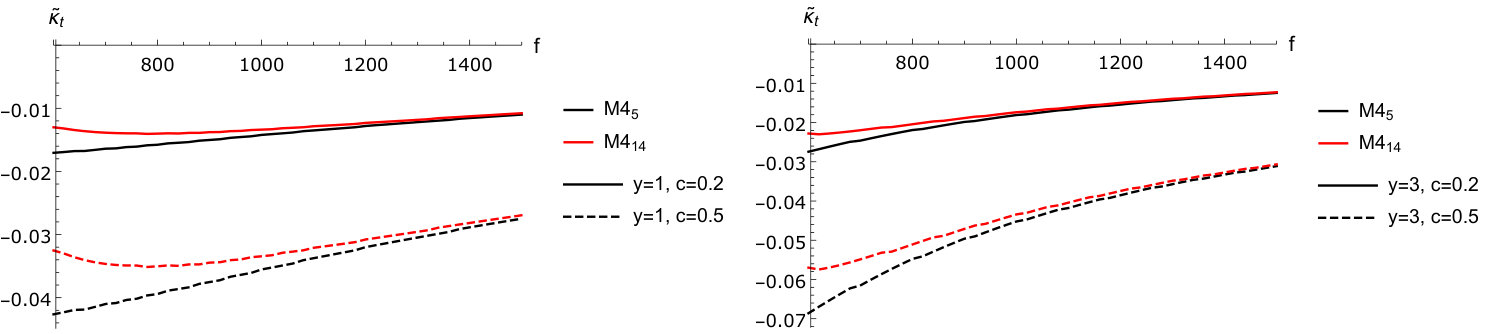 Figure 1
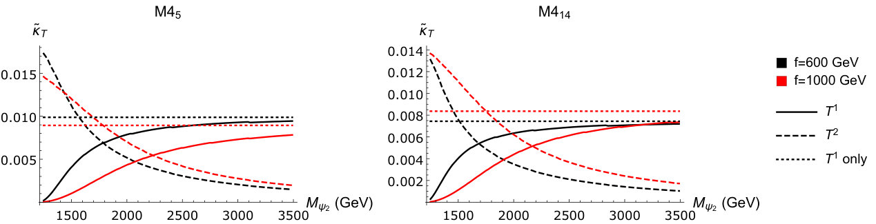 Figure 2
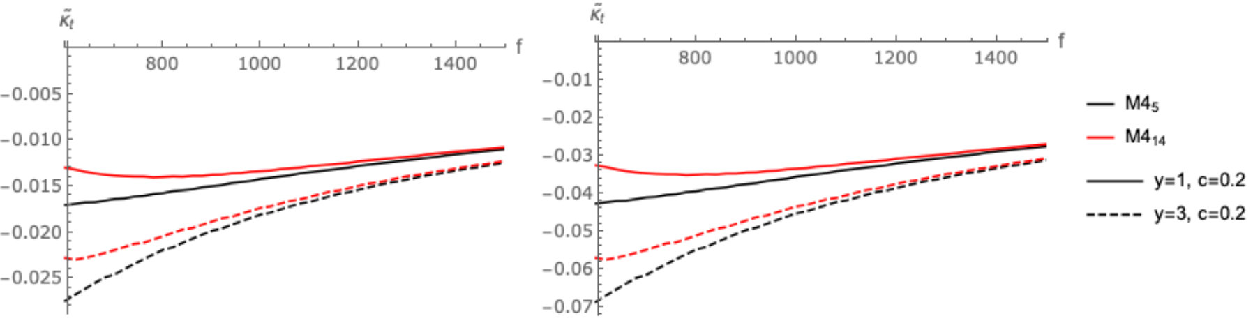 Figure 3
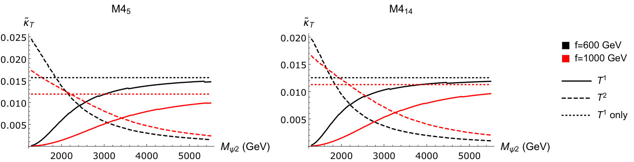 Figure 4
 Figure 5
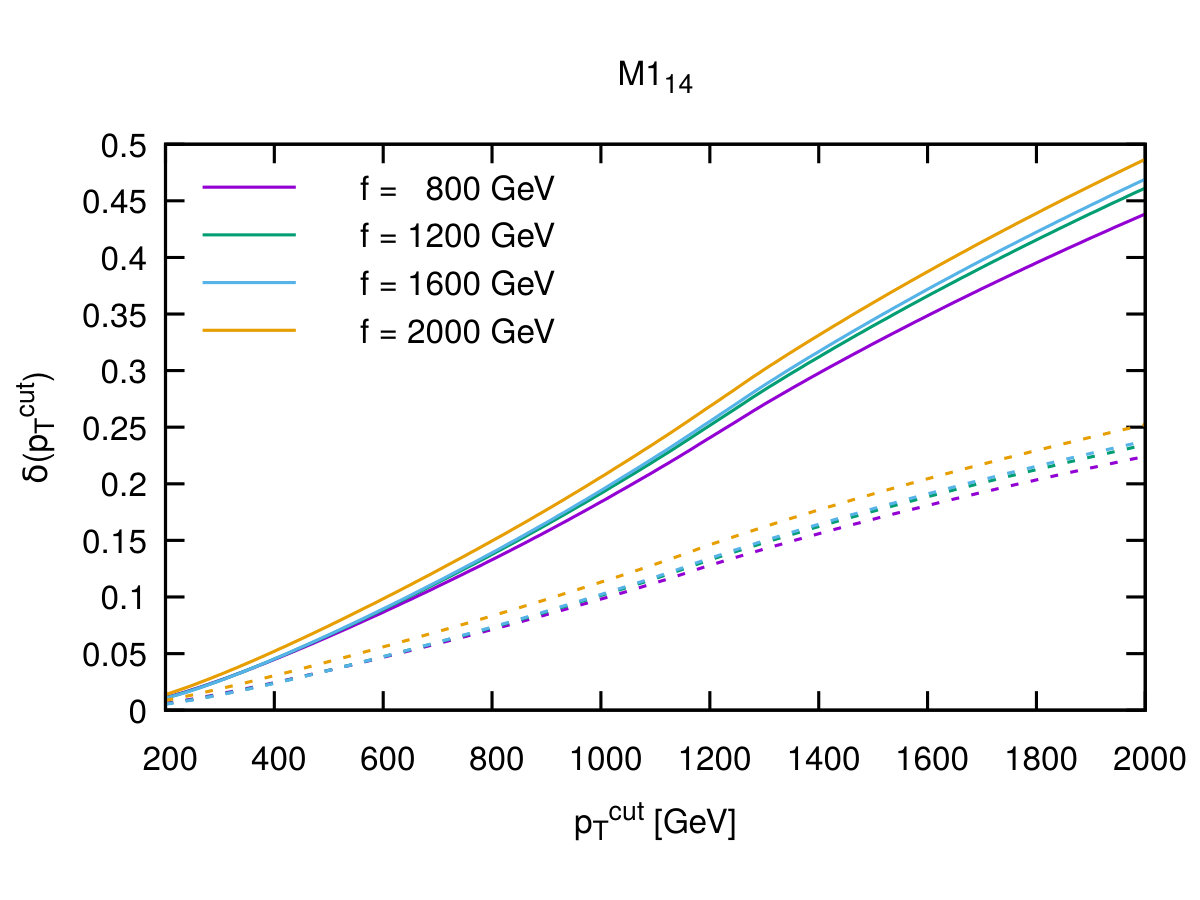 Figure 6
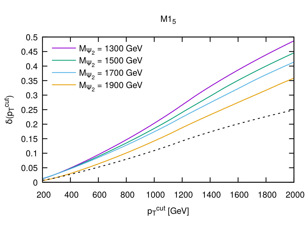 Figure 7
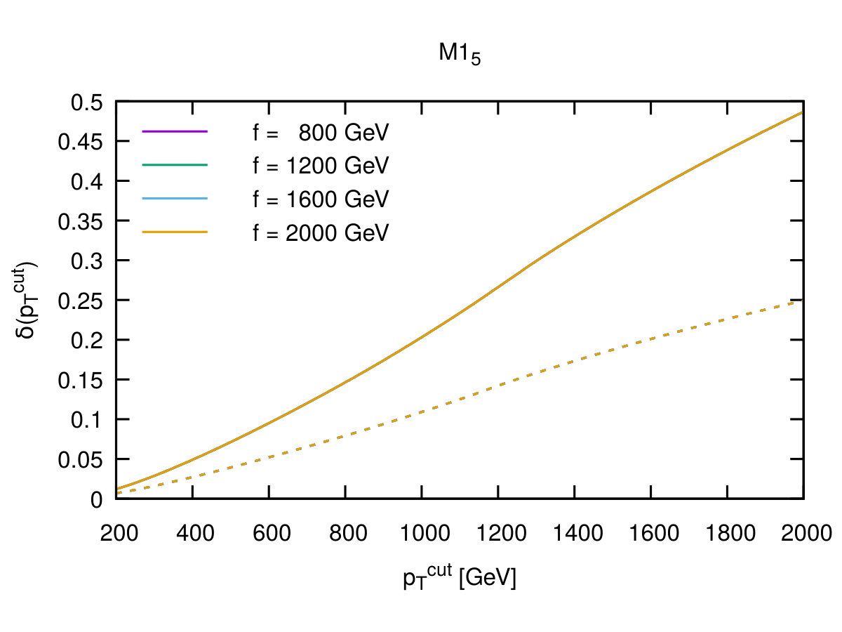 Figure 8
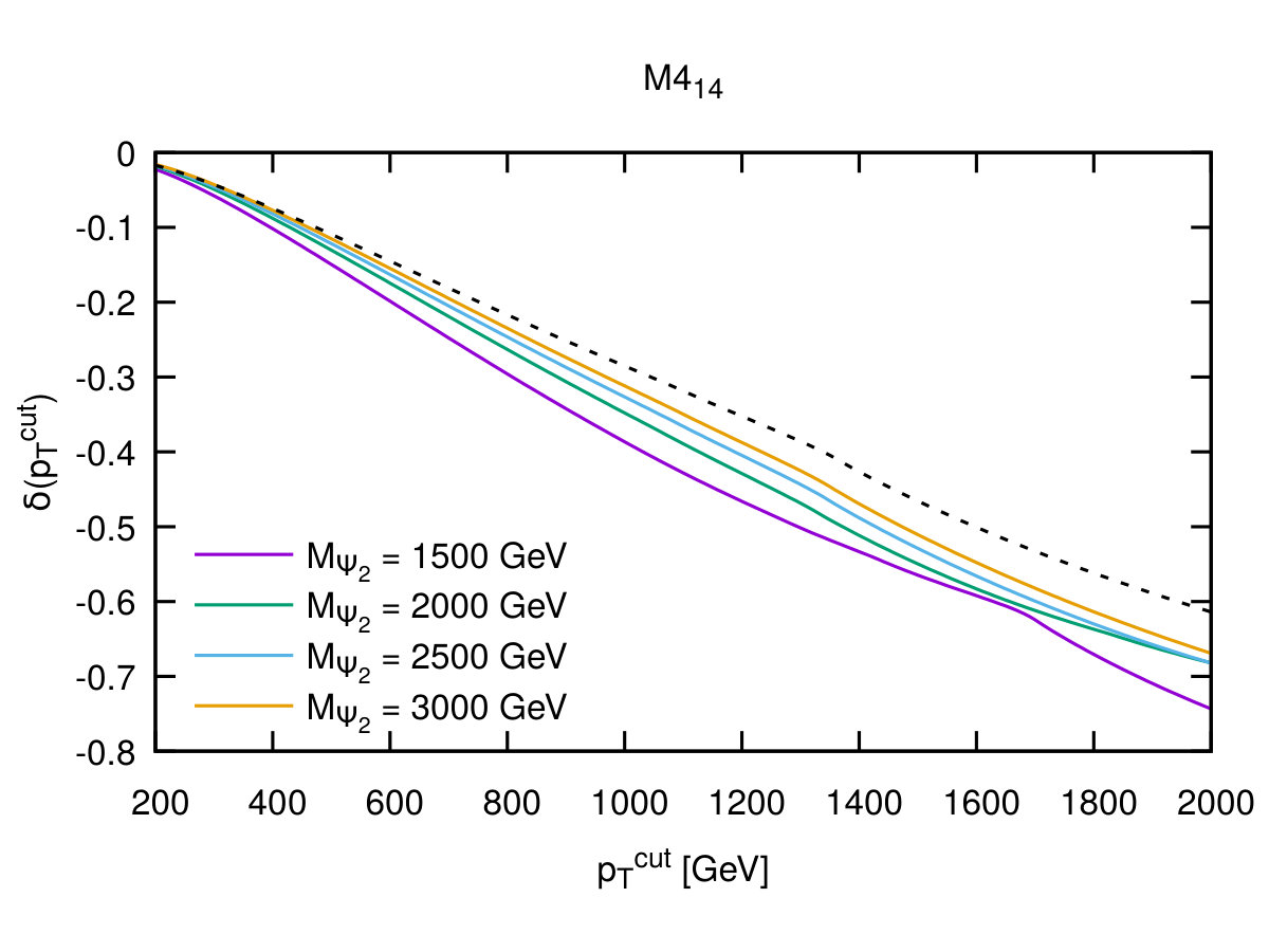 Figure 9
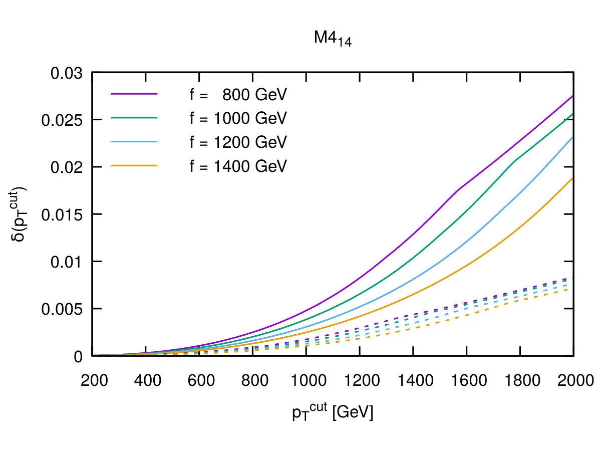 Figure 10
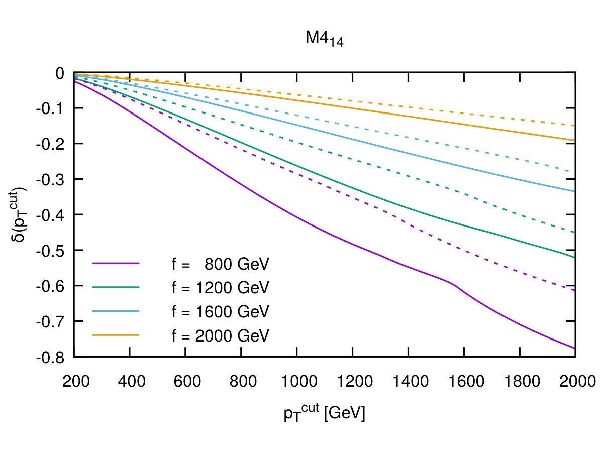 Figure 11
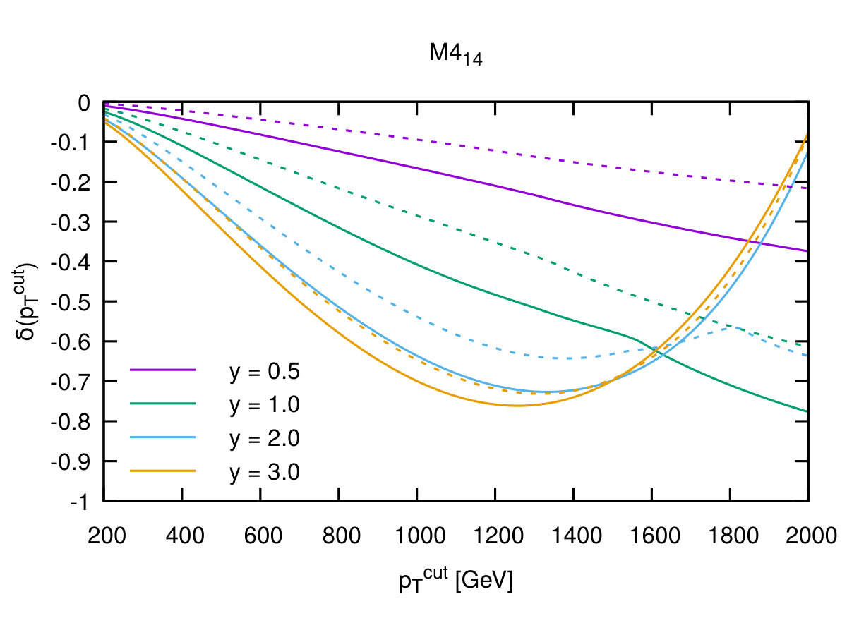 Figure 12
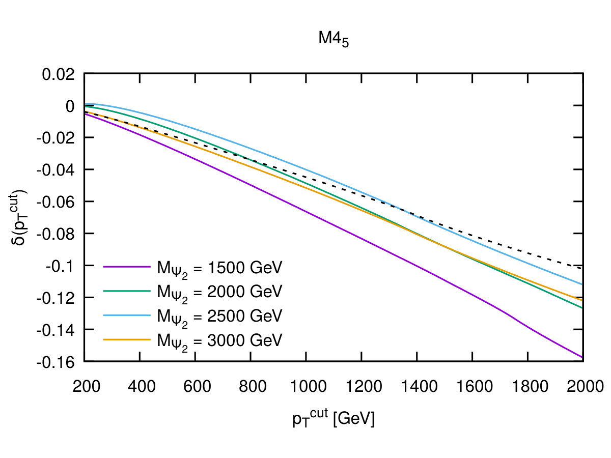 Figure 13
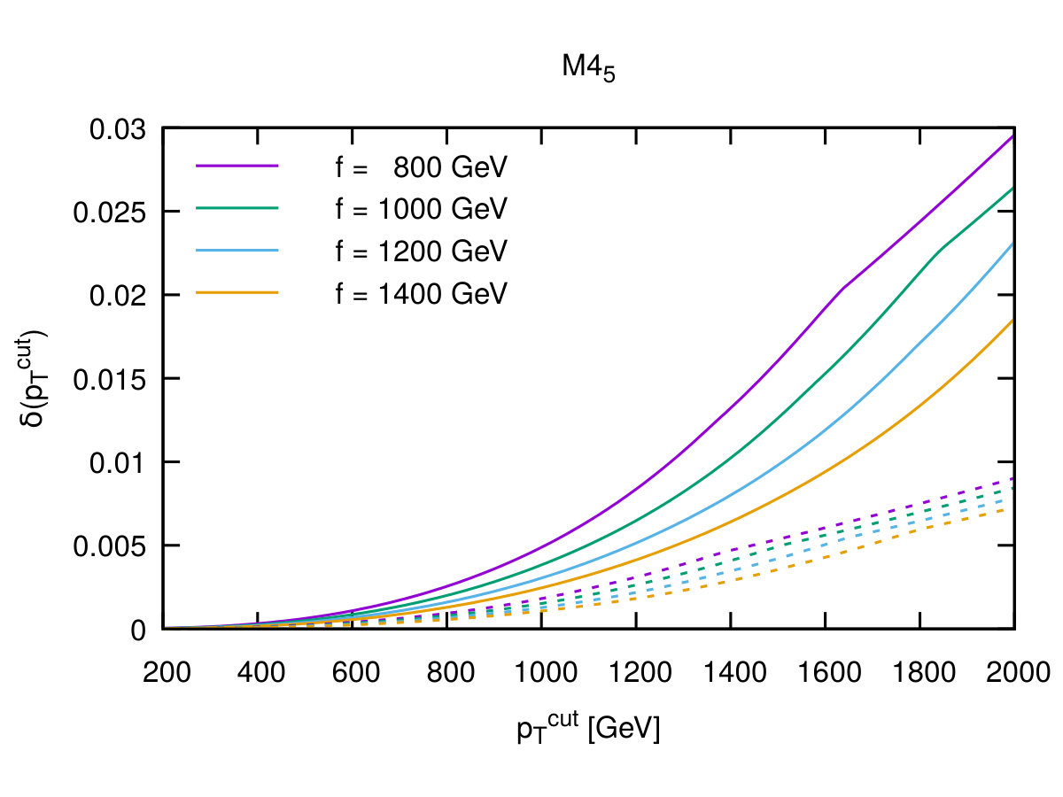 Figure 14
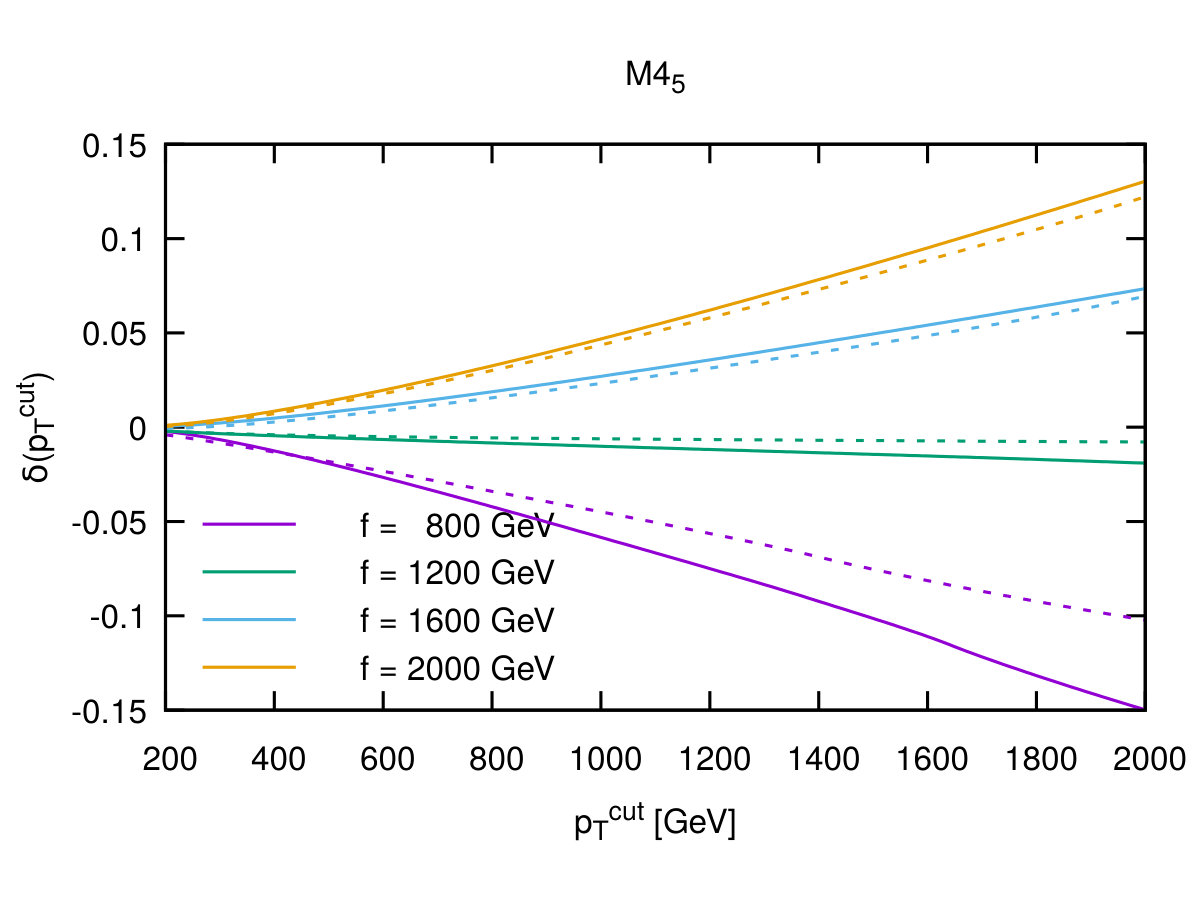 Figure 15
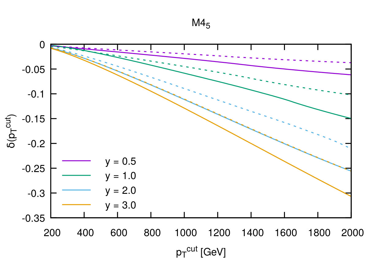 Figure 16
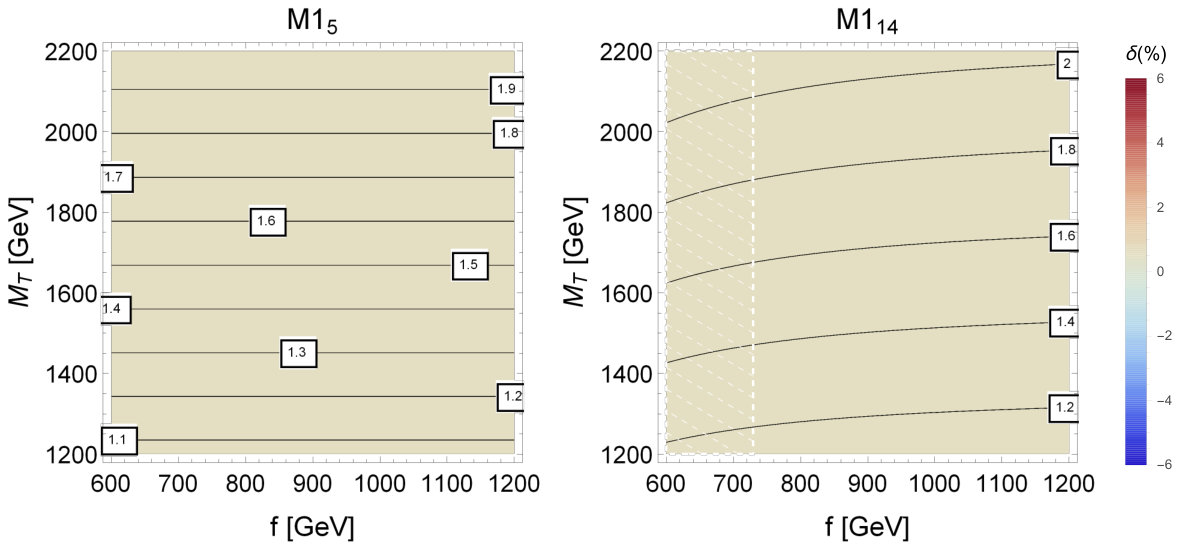 Figure 17
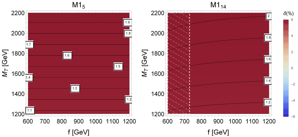 Figure 18
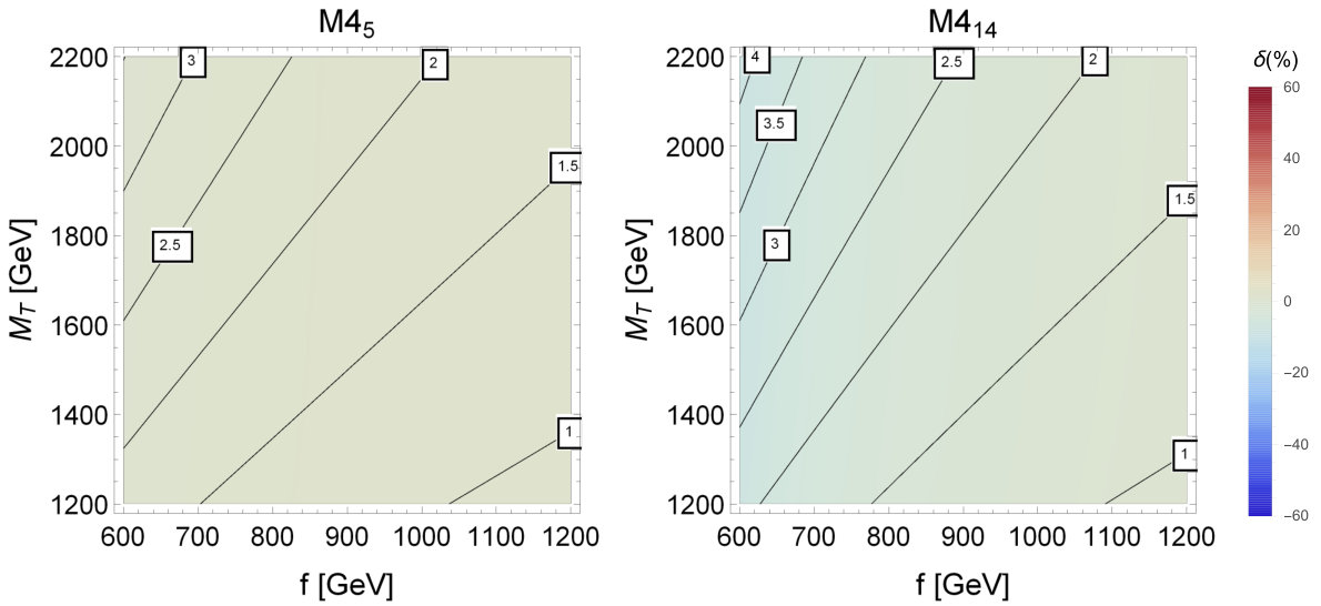 Figure 19
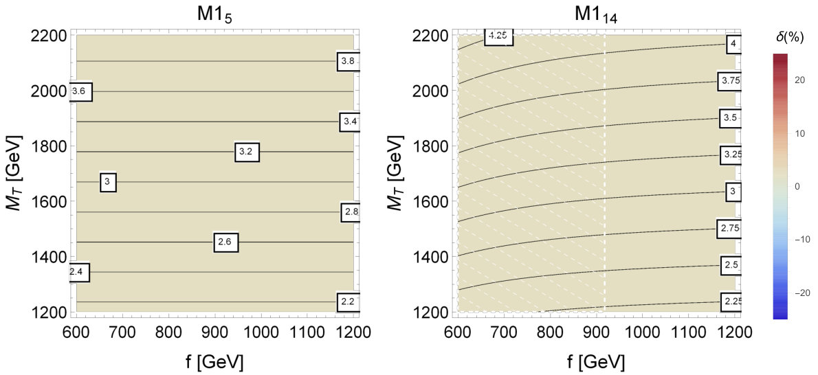 Figure 20
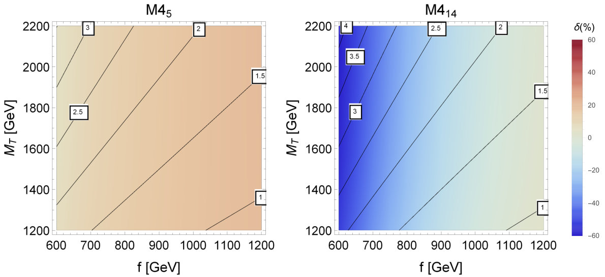 Figure 21
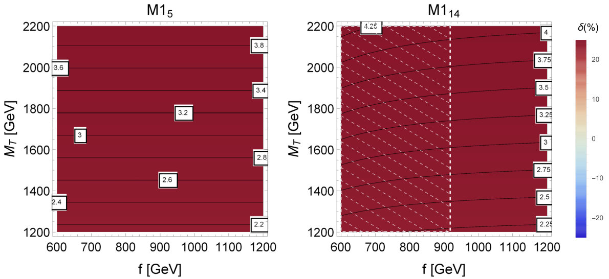 Figure 22
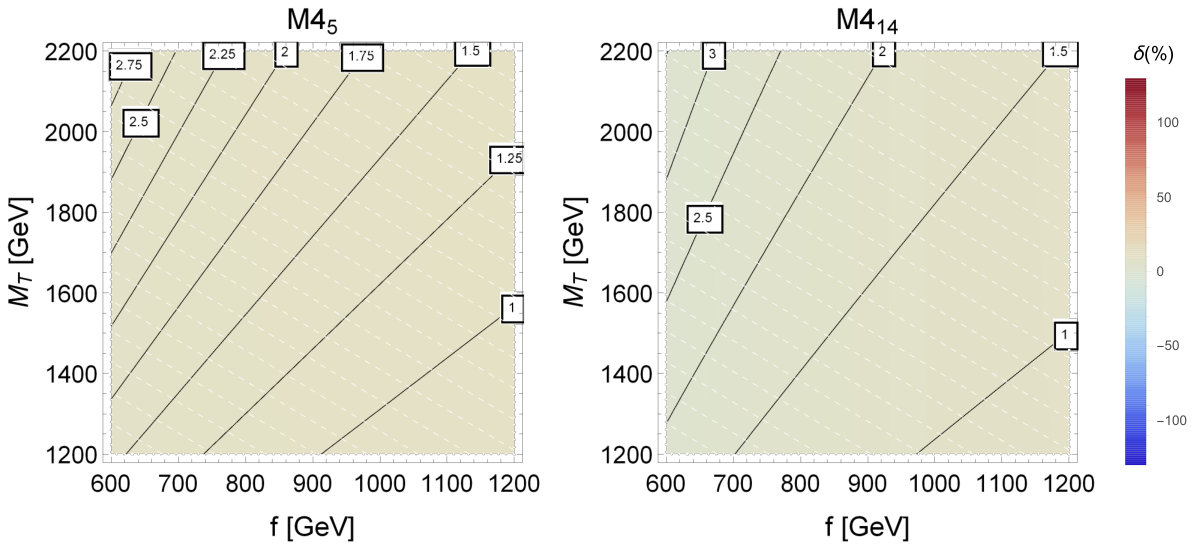 Figure 23
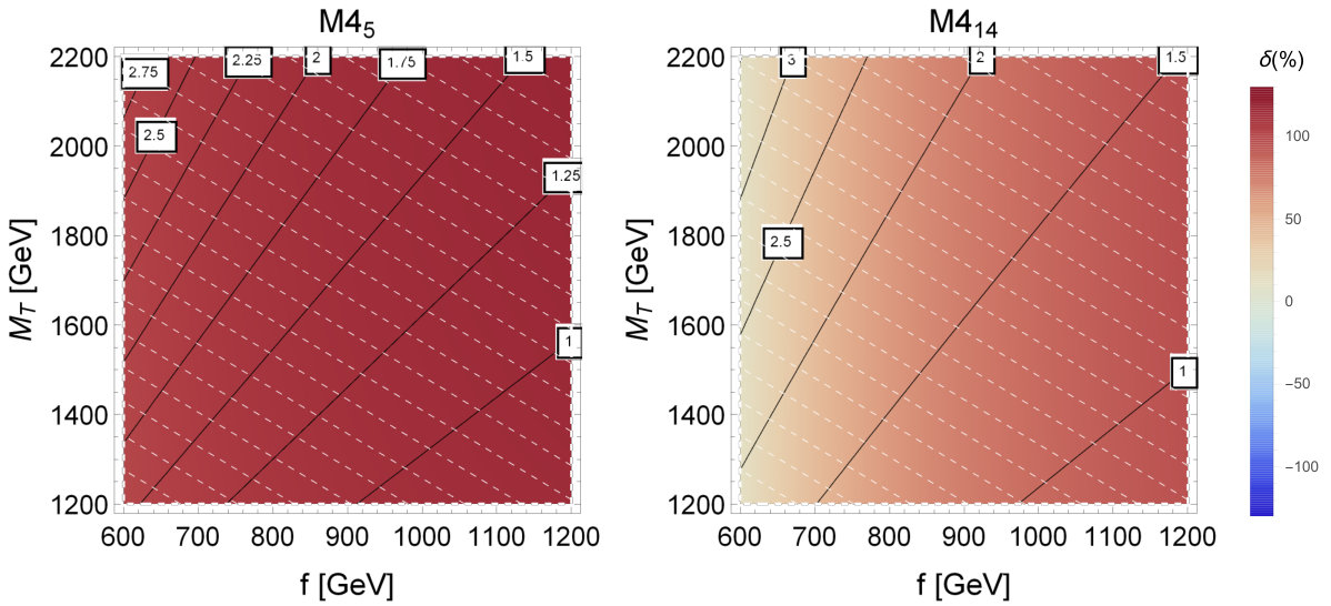 Figure 24
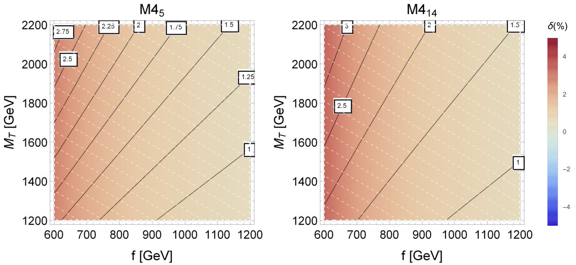 Figure 25
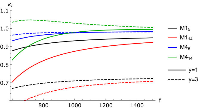 Figure 26
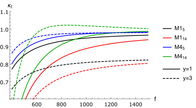 Figure 27
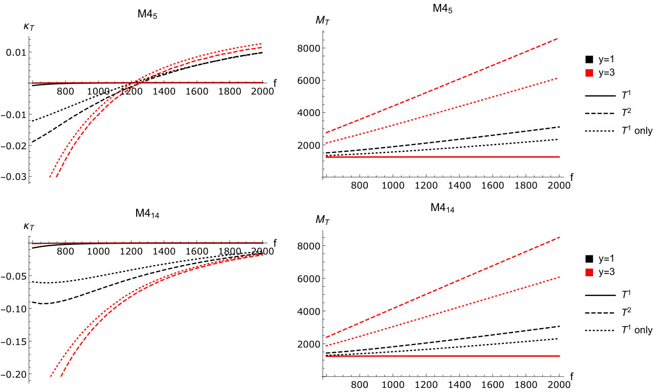 Figure 28
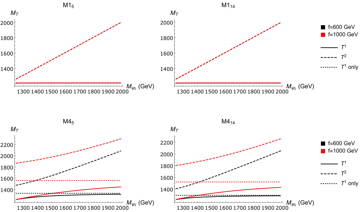 Figure 29
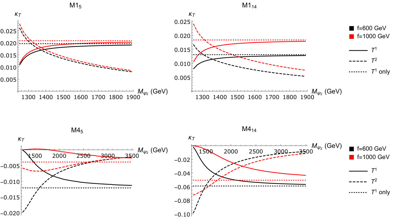 Figure 30
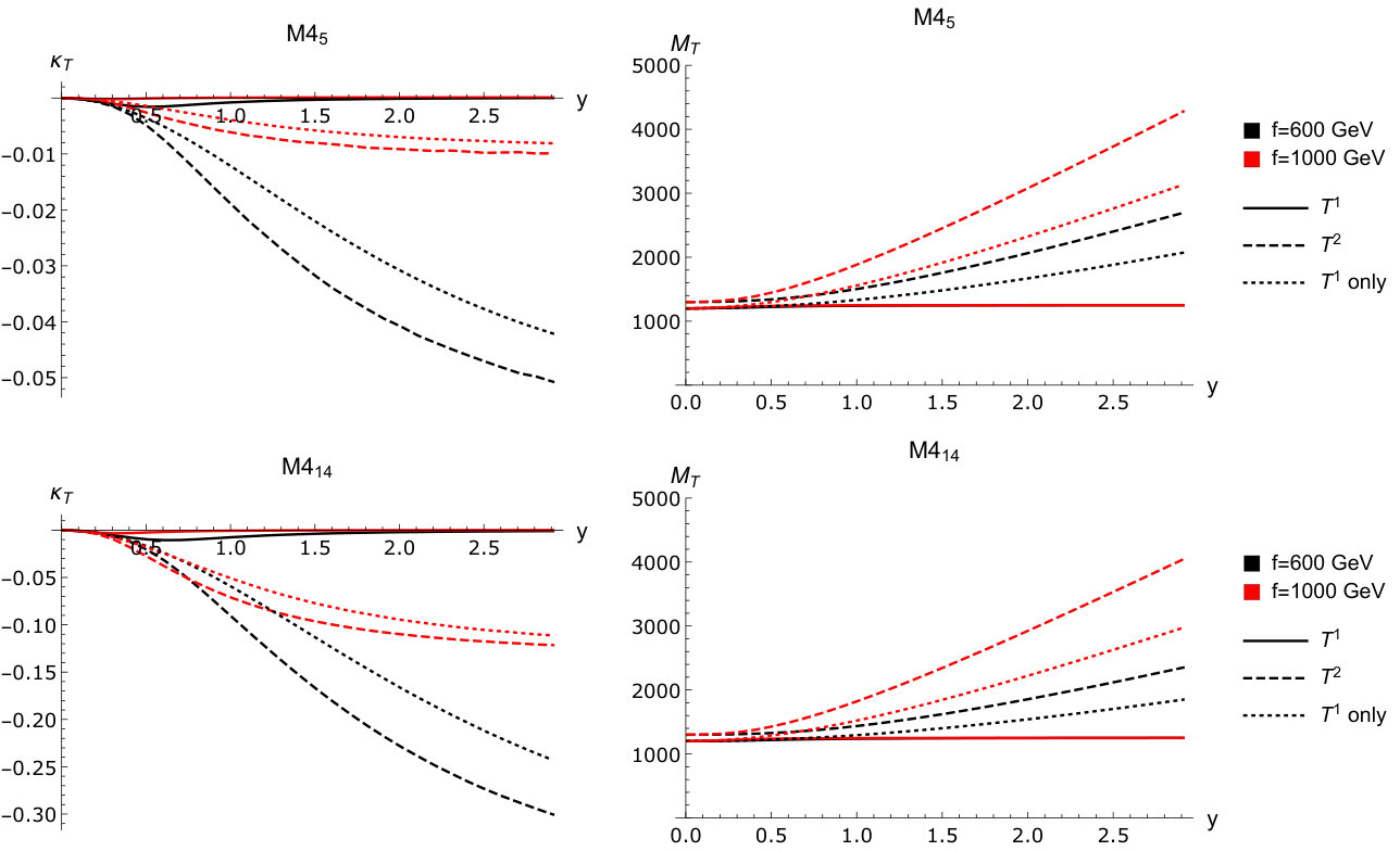 Figure 31
Peer Reviews
No public reviews on file for this paper yet. If you reviewed it on a platform where reviews are public (OpenReview, ICLR, NeurIPS, ICML), you can paste yours below so the community can read it here.
Videos
No videos yet. Explain this paper in a talk, walkthrough, or lecture? Add one.
††institutetext: 1* Department of Physics and Astronomy, University of Sussex, BN1 9QH Brighton, UK
2 Department of Theoretical Physics, Jozef Stefan Institute, 1000 Ljubljana, Slovenia*
Composite Higgs at high transverse momentum
Andrea Banfi1, Barry M. Dillon2, Wissarut Ketaiam1, and Sandra Kvedaraitė1
Abstract
In this paper we explore composite Higgs scenarios through the effects of light top-partners in Higgs+Jet production at the LHC. The pseudo-Goldstone boson nature of the Higgs field means that single-Higgs production via gluon fusion is insensitive to the mass spectrum of the top-partners. However in associated production this is not the case, and new physics scales may be probed. In the course of the work we consider scenarios with both one and two light top-partner multiplets in the spectrum of composite states. We study corrections to the Higgs couplings and the effects that the light top-partner multiplets have on the transverse momentum spectrum of the Higgs. Interestingly, we find that the corrections to the Standard Model expectation depend strongly on the representation of the top-partners in the global symmetry.
1 Introduction
The Standard Model (SM) description of particle physics does not contain a dynamical description of electroweak symmetry breaking (EWSB), or a natural explanation of the vast hierarchies in the Yukawa couplings of the theory. There are many proposed extensions to the SM which provide these explanations and in turn predict deviations in the Higgs properties with respect to what one would expect from the SM description. Thus far the production and decay rates of the scalar resonance discovered in 2012 by the ATLAS and CMS collaborations Aad:2012tfa ; Chatrchyan:2012xdj fit the description of those of the SM Higgs boson, providing constraints on these beyond-the-SM (BSM) models. However, as more data is collected, it is possible that new physics effects could present themselves soon.
Composite Higgs models Kaplan:1983fs ; Kaplan:1983sm ; Georgi:1984af ; Dugan:1984hq ; Contino:2003ve are one particular class of models which provide an elegant description of a dynamical origin for EWSB and of hierarchical Yukawa couplings. These new physics scenarios posit that the Higgs boson is a composite state of some strongly coupled gauge theory with a confinement scale of the order of one TeV. Along with the Higgs boson we expect a plethora of new composite states laying near or above the confinement scale, and we refer to these collectively as the strong sector. The hierarchy between the Higgs mass and the confinement scale is neatly accommodated in the theory when the Higgs field arises as a set of Goldstone bosons generated by the spontaneous breaking of some global symmetry of the UV theory. The different composite Higgs models are labeled by the coset representing the spontaneous symmetry breaking which gives rise to the Higgs doublet, with the minimal models being and Agashe:2004rs ; Contino:2006qr . In this paper we will focus on the latter model because the unbroken global symmetry contains the custodial group, and thus bounds from electroweak precision and the measurements are less stringent Agashe:2006at . Given that the Higgs field is composed of Goldstone bosons, it has no potential at tree-level and thus the electroweak symmetry must be broken radiatively, making the Higgs boson a pseudo-Nambu-Goldstone-Boson (pNGB).
The mechanism at the heart of both EWSB and the Yukawa coupling hierarchies is partial compositeness, through which the SM fermions couple linearly to composite fermions from the strong sector. These couplings necessarily break the global symmetry of the strong sector, because the SM fermions cannot transform as complete multiplets of this global symmetry, and a Higgs potential is generated radiatively. Given that the top quark has the strongest coupling with the Higgs one would rightly assume that this field, and the composite states to which it couples, provide important contributions to the Higgs potential. The composite states that couple to the top-quark through partial-compositeness are known as ‘top-partners’ and in explicit composite Higgs constructions, i.e. those in which the Higgs potential is finite, it is invariably found that the top-partner masses are directly related to the fine-tuning required in the Higgs potential to achieve the observed Higgs mass and vacuum expectation value, with lighter masses corresponding to less fine-tuning. A variety of explicit constructions have been developed over the years, most notably the holographic models Hosotani:1983xw ; Hosotani:1983vn ; Maldacena:1997re ; Witten:1998qj ; Randall:1999ee ; Rattazzi:2000hs ; Huber:2000ie ; Contino:2003ve ; Contino:2004vy . There has also been much success with the discrete site models Panico:2011pw and models employing Weinberg sum rules Marzocca:2012zn . It is well known by now that in order to reduce fine-tuning in the Higgs potential in composite Higgs models light to-partners are generically required. This was first observed in Contino:2006qr and subsequently studied in more detail in Matsedonskyi:2012ym where the relation between the Higgs mass, the top-partner mass, and compositeness scale was understood analytically. In Panico:2012uw the authors confirmed this behaviour for a variety of embeddings of the top-partners in the global symmetry, noting that the case in which the right-handed top quark is composite belongs to a class of minimally tuned composite Higgs scenarios. It has been noted in Croon:2015wba that the holographic models, as studied in this paper, do in fact allow for an alleviation of the tension with light top-partners observed in Contino:2006qr by reducing the UV scale of the 5D model. In the 4D picture this is analogous to a modification in the number of colours in the strongly coupled gauge theory underlaying the compositeness sector. Phenomenological bounds on the masses of new vector-like fermionic states are readily available, the absence of any direct detection of top-partner states at the LHC puts a lower bound on their mass at around GeV ATLAS:2016cuv ; CMS:2017jfv ; CMS:2017wwc ; CMS:2018pma ; Sirunyan:2019tib ; CMS:2018vou ; CMS:2018haz ; Aaboud:2017qpr ; Aaboud:2017zfn ; Sirunyan:2017ynj ; Sirunyan:2017pks ; Sirunyan:2018fjh ; Sirunyan:2018omb ; Aaboud:2018uek ; ATLAS:2018qxs . Through the measurement of Higgs couplings to gauge bosons a direct lower bound on the decay constant of the Higgs field is found to be GeV, depending on the specific model Sanz:2017tco .
In this paper we will investigate the effects that top-partners in composite Higgs models have on the Higgs+Jet production process at the LHC. When studying top-partner phenomenology in composite Higgs models it is necessary to use simplified models to capture the relevant features of the top-partner states without over-complicating the parameter space. In this spirit we follow closely the simplified phenomenological models described in DeSimone:2012fs ; Marzocca:2012zn . The effects of top-partner states on single-Higgs production via gluon fusion have been studied in detail, however in this case the pNGB nature of the Higgs boson leads to a cancellation of new physics effects dependent on the top-partner masses in the production cross-section Kniehl:1995tn ; Azatov:2011qy ; Low:2010mr . To probe the top-partners in gluon initiated Higgs production the produced Higgs must be allowed to recoil off a gluon, and for this the study of Higgs production in association with a jet is useful. This process has been studied in some detail already Banfi:2013yoa ; Grojean:2013nya ; Azatov:2016xik . In this paper we take the study of Higgs+Jet production further in two ways; first of all we show how different top-partner models result in different signatures in the spectra of the Higgs, and secondly we go beyond the simplified models in DeSimone:2012fs and study the effects of a second light top-partner. In the course of this work we also study the effects of CP violating couplings of the top quark and top-partners in the Higgs+Jet process.
In the next section we will introduce the simplified models we use in our analysis and discuss partial compositeness in the top sector of the Minimal Composite Higgs Model (MCHM) based on the coset. After describing the different top-partner states that we have in these models we give a brief overview of the relevant collider bounds and discuss how they constrain the parameter space we study. In section 3 we study the mass spectrum and Yukawa couplings of the top-partners when we have more than one light multiplet. In section 4 we will discuss the main features of single-Higgs production via gluon fusion and in association with a jet, highlighting the differences between the two processes. Finally in section 5 we will present the results of our analysis on each of the simplified models in scenarios with both one and two light top-partner states.
2 Top-partners in the Minimal Composite Higgs Model
The starting point in writing down the MCHM is the assumption that the strongly coupled gauge theory underlying the composite dynamics has a global symmetry, which at the confinement scale is spontaneously broken to . The four Goldstone bosons arising from this symmetry breaking pattern form an fourplet in the coset which we identify with the Higgs field. The fact that this breaking preserves the custodial symmetry has important consequences for the phenomenological bounds on the model Agashe:2006at , as mentioned in the Introduction. Following DeSimone:2012fs ; Marzocca:2012zn we assume that all the SM fields enter as elementary fields with the exception of the right-handed top quark, , which we assume to be a chiral bound state of the strong sector. The gauge fields are coupled to the strong sector through the gauging of the subset of symmetry, with the hypercharge generator being associated with the diagonal generator of plus the generator, i.e. . The SM fermions are coupled to the strong sector through the partial compositeness mechanism, where operators containing SM quarks are coupled to operators of the strong sector. The SM quark doublet cannot fill a complete multiplet without the introduction of additional external states while the states in the strong sector can, thus some of the components of this multiplet will be spurious and lead to explicit breaking of the symmetry.
We will use the standard CCWZ Coleman:1969sm ; Callan:1969sn toolkit to determine the structure of our top-partner effective field theory (EFT) given the coset. These techniques were first used for top-partner studies in Marzocca:2012zn , and for a detailed account of the application of this formalism to the models we employ here we refer the reader to DeSimone:2012fs . The main objects we require in our analysis are the Goldstone boson matrix and the vector used to construct the kinetic term of the Goldstone boson Lagrangian. Under rotations the Goldstone matrix transforms non-linearly as , with and , whereas transforms linearly as a fourplet of . In unitary gauge the Goldstone boson matrix can be expressed as
[TABLE]
where and . When the Higgs is expanded around a vacuum expectation value we take and fix , with , such that the electroweak gauge boson masses are the same as in the SM. We also define , and use the short-hand notation and .
If we now construct top-partner states in representations of we can promote these to representations using the Goldstone boson matrix . As in DeSimone:2012fs , we will study top-partners in either the or representations of , while the SM doublet quarks will be embedded in either a or of . The right-handed top quark will always be defined as a of , since it is being treated as a composite chiral state. The SM left-handed quark doublets in the and the are written in the form
[TABLE]
The right-handed top quark can be embedded in an fiveplet as
[TABLE]
In writing down the effective Lagrangian for the Higgs field, the top quark, and the top-partners, it is useful to also write the vector-like top-partners as embeddings in multiplets. The top-partners in and representations of can be embedded in fiveplets as
[TABLE]
respectively. Embeddings in a of follow similarly. The embedding of the SM quarks ensures that the theory includes the SM doublet with hypercharge and a right-handed top quark with . In fact the hypercharge of the right-handed top quark fixes the charge assignments of all the fermionic fields described above, and the singlet top-partner has the same SM charges as the SM right-handed top quark. However the quarks from the fourplet form two doublets, , has the same SM charge assignment as the SM quark doublet and is an exotic doublet where the subscript denotes the electromagnetic charge.
2.1 The models
In this work we employ simplified models, as outlined in DeSimone:2012fs , which serve to capture the features of light top-partner states relevant for phenomenological purposes. These models are not complete concrete realisations and there is not enough structure to compute a finite Higgs potential or determine the level of fine-tuning present in the Higgs potential. Due to this we will assume that the Higgs mass takes its observed value and that the fine-tuning in the Higgs potential is smaller for smaller top-partner masses. We will however be able to calculate the top quark mass from the mixing between the SM top quark and top-partners and this will serve as a constraint on the parameters of the Lagrangian.
Composite Higgs models predict many new composite resonances of differing spin with masses near the compositeness scale, which we define as . If is sufficiently large one can write down an effective field theory where states above that mass scale have been integrated out. However, in order to obtain a natural EWSB scenario we know that light top-partners are required, therefore it would be natural to suspect that the lightest top-partners have masses which lay below the scale and cannot be integrated out. The approach taken in DeSimone:2012fs and in other simplified models, including those used by the ATLAS and CMS collaborations, assumes that only one top-partner lays below the scale . Allowing more than one light top-partner could drastically change the collider phenomenology as the possibility of additional cascade decays opens up and the relationship between the top-partner masses, couplings, and changes. We will discuss the current collider bounds in section 3.3 however this will not be the focus of the current paper.
The effective field theory for the models we use here are constructed using the same power counting rules as in DeSimone:2012fs which in turn follows the ‘SILH’ approach Giudice:2007fh . Given the choices of top-partner states and SM quark embeddings described in the previous section we see that there are four top-partner models to study: , and .
With a light top-partner transforming as a of and the SM left-handed top-bottom doublet embedded in a of the relevant effective action for the SM plus the top-partner, after the states heavier than have been integrated out, is
[TABLE]
where the embedding of the top-partner states is assumed. The in Eq. (2.1) is the coupling that mixes the elementary and strong sectors, and are expected to be coefficients arising from integrating out the heavier states. Notice that the coupling proportional to does not carry a dependence since is treated as a composite state. Fixing to unitary gauge and expanding the Higgs field around its vacuum expectation value the following mass matrix is found for the top and top-partners
[TABLE]
An orthogonal rotation of the and states reduces the above mass matrix to a mixing between just one linear combination of the top-partners, and leaves the kinetic and vector-like mass terms invariant. If we did not do this rotation now then it would simply be part of the mass matrix diagonalization done later. This transformation can be written as
[TABLE]
and the resultant mass matrix is
[TABLE]
with the state is now decoupled from the top quark and the Higgs. Upon diagonalising this mass matrix the mass of the top-partner gets shifted away from the vector-like mass, however the masses of both the and state remain degenerate at .
For a light top-partner transforming as a of and the SM left-handed top-bottom doublet embedded in a of the relevant effective action is
[TABLE]
where is defined as the direct product of the breaking VEV, , and . In this way the invariant in the Lagrangian can be written as , in accordance with DeSimone:2012fs . We also use an analogous definition of . Because the top-partners transform in a of the particle content here is the same as in the model, however the mass matrix differs slightly due to the embedding of the SM doublet,
[TABLE]
Analogously to the previous model we can also rotate the top-partner states such that only one of the top-partners couples to the SM doublet and the Higgs, with the transformation being
[TABLE]
leaving the resultant mass matrix as
[TABLE]
The state has decoupled in the same way as in the model and has a mass degenerate with the exotic top-partner.
For a light top-partner transforming as a of and the SM left-handed top-bottom doublet embedded in a of the relevant effective action is
[TABLE]
where the term proportional to is now absent. With singlet top-partners we only have one top-partner state with charges equal to that of the right-handed top quark. The mass matrix in this case is simpler than with fourplet top-partners, and is written as
[TABLE]
For a light top-partner transforming as a of and the SM left-handed top-bottom doublet embedded in a of the relevant effective action is
[TABLE]
where the singlet composite states are embedded in representations of when coupled to the SM doublet. The mass matrix is similar to the case,
[TABLE]
2.2 Additional light top-partner multiplets
Introducing additional light top-partner multiplets can be done in a straightforward way. To keep the models simple we will assume that all top-partner states couple to the SM with the same strength, with their masses determining their influence on the top mass and Yukawa coupling. We label our top-partner multiplets as and , and their masses as , whereas the components of these multiplets we label as , , , .
Introducing additional multiplets in the and is straightforward since we are dealing with singlet top-partners. For example the mass matrices for these models with one additional singlet each can be written as
[TABLE]
When the top partners are in fourplets all we need to do is to rotate each pair separately such that only one linear combination of quarks from each multiplet couples to the top quark and the Higgs. For one additional top-partner in the fourplet models this can be done using the orthogonal transformations
[TABLE]
for with , and
[TABLE]
for with . Adding more top-partners requires analogous rotations of the form above. The important point is that we can completely decouple the states from the top quark and the Higgs irrespective of how many top-partners we have. The mass matrices for these models with one additional light top-partner can then be written as
[TABLE]
One can see from this construction that adding an arbitrary number of light top-partners can be implemented in a straightforward way. There is also no need for the light top-partners to be in the same representation as each other, one could just as well have a light singlet and fourplet in the spectrum and there would be no extra complication.
3 Mass spectrum and Yukawa couplings
The purpose of this section is to study how the masses and Yukawa couplings vary with the input parameters for scenarios with both one and two light top-partner multiplets in each of the scenarios discussed in the previous section.
The first thing to discuss is the effect of the operators in Eq. (2.1) and Eq. (2.1) which are preceded by the coefficients. After writing the term in unitary gauge we have
[TABLE]
and thus the top-partners have a derivative coupling with the Higgs boson. Via a field re-definition we can recast this derivative coupling to a CP-odd Yukawa term, which scales as , plus operators that involve higher powers of the Higgs boson field, or different fermionic fields, and hence are not relevant for single-Higgs production.
The general EFT Lagrangian that contains the interactions between the top quark and the charge top-partners which mix with the top quark is
[TABLE]
where the sums over indicate sums over top-partner multiplets, and in this work we will consider at most two multiplets. The mixing of the bottom quark with the composite sector is assumed to be small therefore we do not include the bottom partners in the EFT. The ’s are defined such that in the SM we have , and . The CP-odd couplings in the second line of Eq. (3) will only exist for the and models, and will be functions of the mixing angles and .
3.1 One light top-partner multiplet
In the case where we have only one light top-partner multiplet the Yukawa couplings in the mass eigenbasis can be written down analytically. In general, the mass-mixing matrix can be written in the form
[TABLE]
diagonalization of the matrix is achieved via a double rotation with left-handed and right-handed mixing angles and respectively. This gives us the mass eigenstates with top mass and top-partner mass , and consequently a relation between and the parameters :
[TABLE]
where the two mixing angles are related through
[TABLE]
It is also useful to have expressions for the mixing angles in terms of the inputs ,
[TABLE]
Although is obtained as a result of diagonalising the mass matrix, we fit the top mass using , and so it makes more sense to trade this to take as the input. From this we can deduce that
[TABLE]
In each of the models we have computed the Yukawa couplings of the top and top-partner to be
[TABLE]
The CP-odd coefficients can be calculated from the interaction
[TABLE]
Since this term depends only on the fluctuation of the Higgs field , we can diagonalise the mass matrix independent of it. After doing that, we find
[TABLE]
where we have neglected terms which mix the states in the mass eigenbasis because these terms do not contribute to Higgs production. Now we perform the field redefinitions
[TABLE]
with to be determined in such a way that the Lagrangian does not contain any terms linear in . In this way, the coupling of and to the Higgs derivative are recast into couplings to higher powers of the Higgs boson and CP-odd Yukawa couplings described by
[TABLE]
The addition of more light top-partners in the model will prevent us from obtaining simple analytical solutions such as the ones above, and the is certainly spoiled.
The bottom quark mass is also generated via partial compositeness, although the mixing of the bottom quark with the composite sector is much milder and the right-handed bottom is certainly not composite. The bottom quark Yukawa couplings are shifted by the same factors of as the top quark, and we can assume that the mixing angles with the composite sector are negligible. Therefore we have only two scenarios for the bottom quark, and . Given that the CP-odd terms are also proportional to the mixing with the composite sector, these can also be taken to be absent for the bottom quark.
3.1.1 Perturbativity and relevant limits
Before discussing some relevant limits of the couplings in eqs. (28)-(32), we investigate which values of , and correspond to values of the mixing paramter that are in the perturbative regime, which we take to be DeSimone:2012fs . To do this, it is useful to re-write the off-diagonal term in terms of a single mixing-angle. Using the relations
[TABLE]
we obtain
[TABLE]
We now want to assess what values of the top-partner masses and mixing angles are consistent with the perturbativity of the interaction terms mixing the top with the vector-like quarks. The perturbativity bound restricts parameters in a different way for singlet and fourplet models, due to the different scaling of with respect to and . For singlet models we have that , thus, for moderate mixing angle and , Eq. (34) implies that . The only possibility to have very large top-partner masses is then to make the angle , and hence , increasingly small. This is a physically sensible limit, because it means that a very heavy top partner essentially decouples. This feature occurs irrespectively of the value of . In the case of fourplet models we have that , thus large values of top-partner masses and moderate mixing angles are still consistent with perturbativity, provided is sufficiently large. These basic considerations show that simplified models determined just in terms of a mixing angle and the mass of a top-partner may not result from a perturbative composite Higgs model. Therefore, in the following sections, whenever we fix mixing angle and top-partner mass, we will always compute the corresponding value of and we will exclude all values of parameters that are not consistent with perturbativity bounds.
The perturbativity bounds we have described do not allow us to take the mass of one top partner to infinity by fixing all other parameters. We can instead take the limit within perturbativity bounds, in which case we have:
[TABLE]
and all CP-odd couplings vanish. For fourplet models, this corresponds to the limit considered in Banfi:2013yoa . Note that, for singlet models, perturbativity restricts the possible values of even for , whereas for fourplet models, this limit corresponds to , with fixed. In this limit, further constraints on the mixing angle are posed by experimental bounds on Aaboud:2018urx , which set the lower bound . This excludes for singlet models, and for fourplet models. For finite , this bound is more stringent for singlet models, because . Fourplet models are less constrained due to cancellations occurring between two different contributions (see eqs. (28), (28)).
3.2 Two light top-partner multiplets
In the case of two top partners and , we take a different approach with respect to the single top-partner case, in that we study the relationship between the fundamental parameters of each model (i.e. the vector-like masses, the couplings and the decay constant ) and the physical top-partner masses and Yukawa couplings. In particular, we take as free parameters , as well as the CP-odd couplings, with being used to fix the top quark mass to GeV.
In Figures 1 and 2 we plot the masses and Yukawa couplings of or as a function of the heavier vector-like mass for GeV, , and GeV. In each plot we also show the masses and couplings of a single top partner (labelled only), corresponding to the same values of and , and .
We stress that, everywhere, is the lighter top partner. The first thing we notice when looking at Figure 1 is that, in the singlet top-partner models, there is almost a degeneracy between the vector-like mass and the mass of the state. There is also no difference between the GeV and GeV scenarios for the singlet models, this is because in these models the mass matrix is largely insensitive to , a feature not shared by the fourplet models. In fourplet models instead, this occurs only as one of the vector-like masses is made much larger than the other. Also, when considering fourplet models, we should keep in mind that are in fact the masses of the and states. Therefore, for , has the same mass as and .
The behaviour of the Yukawa couplings shown of Figure 2 presents some interesting features, as we see that, in some circumstances, the heavier top-partner can have a larger coupling to the Higgs than the lighter one. This effect is only present when when is close to , and as the gap between the two masses widens we can see the heavier top-partner beginning to decouple from the Higgs and the Yukawa coupling of the lighter top-partner approaching the value expected when only one light top-partner is present. For the fourplet models, in particular , there is a large region in which the heavier top-partner holds the dominant coupling to the Higgs boson. What is striking here is that the coupling of the lighter top-partner to the Higgs boson can be suppressed if there is a heavier top-partner of the same charge with a slightly heavier mass.
We then direct our attention to the top quark Yukawa couplings in Figure 3, and we plot their values as a function of the compositeness scale in the interesting case of quasi-degenerate vector-like masses GeV and GeV, and for two different values of . In the case of a single top-partner, we set . As can be seen from Fig. 2, this represents very well the case of two top partners when . We observe that, except for small values of , the top-quark anomalous Yukawa coupling depends very mildly on since at large the corrections are dominated by the mixing angles between the top and the top partners. The dependence on is similar both for one top partner (the left panel of Figure 3) and for two top partners (the right panel of Figure 3). In particular, the -dependence is much stronger for singlet models than for fourplet models, with a 30% suppression with respect to the SM for larger values of . As expected, for low values of we see drastic deviations from the SM value, particularly in the singlet models. In fact, the recent observation of Higgs production in association with a top-antitop pair by the ATLAS experiment Aaboud:2018urx sets the lower bound , which excludes the singlet models with in both the one and two top-partner cases for the whole range of values of shown. Therefore, in the following, when comparing singlet and fourplet models, we will restrict ourselves to the case .
In order to show how the composite-elementary mixing parameter affects the physical masses and Yukawa couplings we have plotted them in Figure 4 for the and models with GeV and GeV. The first feature to note is the behaviour at small : in this region the Yukawa couplings of the top-partners become very small and the masses approach . The reason for this is because we are decoupling them from the top quark and the Higgs, while the top quark mass is being kept at its observed value by the coupling. As increases, the differences between and grow, the mass of the lighter state stays close to the vector-like mass and the mass of the heavier state is enhanced. The behaviour of the Yukawa couplings as varies is less trivial and depends strongly on the value of .
In Figure 5 we show how these masses and couplings depend on the decay constant . We have again used the and models as an example, with GeV and GeV, or , and plotted the anomalous Yukawa couplings and masses as a function of . Interestingly, we see that one top-partner effectively remains light as is increased and decouples from the Higgs. The other increases in mass as increases, and its Yukawa coupling approaches that of the top-partner in the single top-partner case. We should note that, as is increased, the ratio becomes small and indicates that the Higgs potential will require more fine-tuning to reproduce the observed Higgs mass and vacuum expectation value.
Lastly, we need to study the couplings of the top-partners to the derivatives of the Higgs in the and cases, which with two top-partners these can be written as
[TABLE]
with
[TABLE]
At this point, we can calculate the interactions between the quarks and the Higgs derivative in the mass eigenbasis by rotating the matrix with the rotations required to diagonalise the mass matrix. In the mass eigenbasis we denote , where is the orthogonal matrix that diagonalises the right-handed side of the top-partner mass matrix, and the couplings relevant for Higgs production via gluon fusion are the diagonal elements. Just as in the case with one top-partner we can perform field redefinitions which recast the diagonal couplings of the quarks to the Higgs derivative into couplings to higher powers of the Higgs boson plus a set of CP-odd Yukawa couplings given by
[TABLE]
It is also useful to see how the CP-odd couplings scale as a function of the input parameters.
In Figures 6 and 7 we plot the CP-odd top and top-partner Yukawa couplings, respectively, in a scenario in which the parameters determining the CP-odd couplings are universal, i.e. . For the top, we examine the dependence of the CP-odd coupling on for different values of and , and for the top-partners we examine the dependence on the vector-like masses , with and two different values of . Note that when we take one top-partner mass to be very heavy, that top-partners CP-odd coupling diminishes, and we find that the CP-odd couplings of the top quark and the light top-partner are equal and opposite, as in the case with one top-partner. This same behaviour occurs in the CP-even Yukawa couplings as the vector-like masses are varied.
3.3 Brief summary of experimental bounds
The first experimental constraint to mention is that on the decay constant , which through the analysis in Sanz:2015sua is constrained to be larger than GeV. These bounds are derived from Higgs decays to vector bosons and Higgs production. Recent bounds on top-partner masses have been obtained through analyses at TeV by the ATLAS collaboration ATLAS:2016cuv ; CMS:2017jfv ; CMS:2017wwc ; CMS:2018pma ; CMS:2018vou ; CMS:2018haz ; Aaboud:2017qpr ; Aaboud:2017zfn ; Sirunyan:2017ynj ; Sirunyan:2017pks ; Sirunyan:2018fjh ; Sirunyan:2018omb ; Aaboud:2018uek ; ATLAS:2018qxs . The first point to note is that these analyses only consider the presence of one light top-partner state, and thus these bounds are relevant to our lightest state. Including heavier states opens up possibilities for much more intricate signatures involving cascade decays. The lower mass bounds on the and partners from the fourplet models are quoted at GeV, and the lower mass bound on for singlet models is quoted at GeV. However, the latter bound assumes that Br. These bounds are weakened if one considers sizeable branching ratios into multiple channels. More interesting and intricate signatures arise in twin Higgs models Chacko:2005pe ; Chacko:2005vw ; Chacko:2005un which have QCD-like dark sectors with Higgs portal couplings to the SM. Much work has been done in developing these models Craig:2015pha ; Craig:2016kue ; Barbieri:2016zxn ; Geller:2014kta ; Serra:2017poj ; Csaki:2017jby ; Dillon:2018wye and studying their phenomenology Burdman:2014zta ; Curtin:2015fna ; Chacko:2015fbc ; Ahmed:2017psb ; Chacko:2017xpd . Translating these collider constraints into bounds on the top-partner models presented in the previous sections is beyond the scope of this paper, and in our analyses we will use a lower limit of GeV for the lightest vector-like mass.
Constraints on the and parameters have been derived from electron and neutron Electric Dipole Moment (EDM) experiments Panico:2017vlk . These results indicate that with the top-partner masses at the TeV scale, the imaginary values of these parameters are constrained to lay . It is not the goal of the present paper to study the effects of these parameters on the EDMs, therefore we will simply constrain in our work. Future electron EDM experiments will introduce much more stringent constraints on these parameters. The remaining parameter space that we wish to study in this paper is summarised by , , and .
4 Higgs production
4.1 Total Higgs cross section
It is well known that the production cross-section of the Higgs boson via gluon fusion is insensitive to the mass spectrum of top-partners in composite Higgs models. This low energy theorem arises due to the pseudo-Goldstone boson origin of the Higgs field in composite Higgs models. This insensitivity has been explored in many studies. In Low:2010mr , the effects from new coloured fermions in composite Higgs models to gluon fusion Higgs production, along with other less transparent effects from new physics, were studied by means of an effective Lagrangian. The new physics effects were inspected by analysing the following higher dimensional operators constructed from SM fields:
[TABLE]
Through an explicit calculation, the authors of ref. Low:2010mr showed that the gluon fusion production rate of the composite Higgs depended only on the decay constant of the model, not on the top-partners mass spectrum.
In ref. Azatov:2011qy , a different approach was used to show the insensitivity of the cross section in composite Higgs model to mass of the top partners. This work considered a generic Lagrangian for a composite Higgs model with a top-partner multiplet in the representation, but their argument holds for all the models discussed in section 2. Consider the contribution to the partonic cross section gluon fusion Higgs production arising from a loop of a number of fermions
[TABLE]
In the above equation, is the Yukawa coupling of fermion of mass to the Higgs boson, is the partonic centre-of-mass energy squared, and is the following function of :
[TABLE]
The contribution to the total cross section from all fermions that are heavier than the Higgs boson can be approximated as
[TABLE]
where is a matrix whose eigenvalues are the masses of the fermions and incorporates the corresponding Yukawa couplings. Furthermore, one can show Azatov:2011qy that
[TABLE]
If we repeat the analysis of ref. Azatov:2011qy for our composite Higgs models we find that, for the models and , we have
[TABLE]
whereas for the models and we obtain
[TABLE]
which are independent of the masses and couplings of the top partners. For a single top partner, the above results can be checked explicitly by computing the Higgs partonic cross section as in Eq. (40) using the Yukawa couplings obtained from Eq. (28).
4.2 Higgs production with an additional jet
In contrast to the case of single-Higgs production from gluon fusion, Higgs production with an additional jet has been shown to have some dependence on the mass of a top partner in composite Higgs models. In ref. Banfi:2013yoa it was shown how the low energy theorem rendering the cross section insensitive to the masses of fermions in the loop no longer holds when the transverse momentum of one of the final states is large. For Higgs plus one extra parton (quark or gluons), this happens at high , the transverse momentum of either the Higgs or the jet. Let us consider one of the partonic subprocesses contributing to , namely . The matrix element , where denotes the helicities of the 3 gluons, for one fermion species in the loop with mass and Yukawa coupling will have a different behaviour according to the size of . For instance, for the amplitude , in the limit we have Banfi:2013yoa
[TABLE]
where are combinations of constants and logarithms that are independent of . On the other hand, for low we have Banfi:2013yoa
[TABLE]
where there is no dependence on the fermion mass, and the result is proportional to what you would obtain for . If we now consider a top quark, with mass and Yukawa coupling , and a top partner with mass and Yukawa coupling , for final states with low the low energy theorem still applies. However, if the transverse momentum is increased to the range , one can approximate the top and top partner contributions to be in high- and low- limits respectively, and obtain, in this kinematic region,
[TABLE]
The expression above is only sensitive to the top mass and Yukawa coupling, and to the top partner Yukawa coupling. The dependencies on the top partner mass will be present if we increase further to the region , where both the top quark and top partner contributions will approximately be in the high- limit form given in Eq. (46). This behaviour of the matrix element was also confirmed numerically Banfi:2013yoa .
5 Higgs plus one jet production at the LHC
The difference between the differential cross section of a SM Higgs and that of a composite Higgs is certainly a very useful probe of the compositeness of the Higgs. This was the observable considered in ref. Banfi:2013yoa . However, two -spectra might be different just by an overall factor because of different total cross sections. Then, as explained in section 4, such difference gives no information at all about the presence of top partners, but only on the compositeness scale, and can be already appreciated by looking at deviations in the total rate for Higgs production. In order to decorrelate the two effects, we prefer to work with ratios of cross sections. Therefore, in this work we propose to employ a net Higgs plus jet efficiency, i.e. the fraction of events for which the Higgs (or at least one jet) has a transverse momentum larger than
[TABLE]
In this case, an overall normalisation of the cross section cancels between numerator and denominator in eq. (49), so that this quantity is most sensitive to the mass of top-partner and the corresponding Yukawa couplings. We now assess the deviation of the one-jet efficiency from its SM value using the variable
[TABLE]
In the above definition, denotes the SM efficiency, while is the efficiency of any of the composite Higgs models studied in this work. As a last remark, in this work we compute using tree-level cross sections only. However, it has recently been found that the K-factor (NLO/LO) for the total Higgs cross section and the Higgs distribution with full top-mass dependence are very similar, roughly a factor of 2 over a wide range of values of Jones:2018hbb . Therefore, we believe that our estimate of will be basically unchanged after the inclusion of higher-order corrections.
5.1 One light top-partner multiplet
We first consider the case of a single top partner in all of the four models considered in section 2. The Yukawa couplings of the top quark and top-partners to the Higgs boson are given, in their analytical form, in Eq. (28). We compute distributions at the LHC with a centre-of-mass energy TeV, the same as in the high-luminosity phase of the LHC. As remarked in ref. Banfi:2018pki , with ab*-1* of integrated luminosity, one can reasonably probe transverse momenta up to TeV. The calculation is performed using a modified version of the program used in ref. Banfi:2013yoa , consisting of an interface of the matrix elements of ref. Baur:1989cm implemented in the program HERWIG 6.5 Corcella:2002jc , with the parton evolution toolkit hoppet Salam:2008qg . All numerical results we present have been obtained by fixing GeV, bottom mass GeV, and using MSTW2008 NLO parton distribution functions Martin:2009iq , corresponding to . We present contour plots for (expressed as a percentage), as a function of the mass of the top-partner and the compositeness scale . The case has been already considered in ref. Banfi:2013yoa . Here we focus on a range of values of and that are not excluded by current measurements, and where there is no specific hierarchy between the two scales.
In the following contour plots, for the singlet models we fix the value of , whereas for the fourplet models we fix the value of . The reason behind this is that, in singlet models, the modification of Yukawa couplings depend only on , which, according to Eq. (25), becomes increasingly large with the top-partner mass. For large values of , the contribution of the top becomes smaller and smaller, and the spectrum is dominated by the contribution of the top-partner. The situation of fourplet models is completely different. There, for large , the Yukawa couplings depend largely on . However, with increasing top-partner masses and finite the Yukawa couplings contain a negative contribution proportional to for the top and for the top partner. It is then more reasonable to fix different mixing angles for different representation of the top partner involved in the models. In addition, in the following contour plots, we also indicate the region where the value of falls below , which is in tension with data, as explained in section 3.1.1. Note that, in the limit , our predictions correspond to those presented in ref. Banfi:2013yoa . In the following, we try then to choose the same parameters as those in ref. Banfi:2013yoa , so as to be able to assess the impact of a finite value of with respect to the limit considered there.
In Fig. 8, we show contour plots of for GeV and for singlet models. Similarly, in Fig. 10, we show the contour plots of for fourplet models with for the same value of .
First, we observe that the deviation from the SM is not large. This is due to the fact that the integrated transverse momentum spectrum is dominated by the lowest values of . There, the top still behaves as a heavy particle in loops, therefore the cancellation between top and top-partner contributions is still at work. Nevertheless, there is a very different behaviour for singlet (Fig. 8) and fourplet (Fig. 10) models. For singlet models, the deviation from the SM mildly increases as is increased. For fourplet models the deviations increases with increasing . This behaviour arises since negative contributions from the Yukawa coupling due to and become smaller as is increased. Note that, for , these negative contributions dominate for small values of , and one gets negative interference between the contribution of the top and the top partner. In these, and all remaining contour plots, we draw solid lines that correspond to fixed values of the coupling , so as to highlight whether the corresponding choice of parameters correspond to a perturbative composite Higgs model. We recall that perturbativity requires . In this respect, we observe that, for singlet models, we cannot legitimately probe top-partner masses above GeV. For fourplet modes instead, our choice of parameters leads to predictions that are almost always within the perturbative region.
We now keep the values and increase to GeV. The corresponding contour plots are shown in Figs. 9 and 11, again as a function of and .
The values probed here are high enough to break the cancellation between the contribution of a top and a top-partner in loops. This is why, for singlet models, we observe huge deviations from the SM. For fourplet models, we note, again, that the deviation decreases with decreasing . This is again due to the fact that for smaller , the negative contribution to the Yukawa couplings due to and becomes more important, and vanishes for . The most striking feature occurs for at small values of , where one sees a large negative interference between top and top-partner contributions.
To have a perfect parallel with ref. Banfi:2013yoa we should repeat the same analysis for . Unfortunately, singlet models with are outside the perturbative regime. Therefore, we can only consider fourplet models with . Contour plots with GeV are shown in Fig. 12
Here the deviation from the SM is again moderate, for the same reasons as the corresponding case with . Also here, is bigger so the negative contributions to the Yukawa couplings proportional to and become less important. Finally, for fourplet models we consider the case GeV, and , whose contour plots are shown in Fig. 13.
The fact that is larger actually prevents the negative contributions from taking over. Therefore, the contribution of the top quark in the loops becomes smaller than those with the top-partner, giving a sizeable deviation with respect to the SM.
We now consider the CP-odd contributions induced by the couplings and in Eq. (32). They exist only for fouplet models and, due to the fact that they cannot interfere with the SM, they are very small. For the values of we consider, their contribution is at the sub-percent level, except for and GeV, where one gets an additional deviation of a few percent with respect to the SM. The corresponding contour plots are shown in Fig. 14.
In order to have an extra example of deviations one might expect for singlet models, we analyse the case where . Contour plots with GeV are shown in Fig. 15, and those with GeV are shown in Fig. 16. Comparing these two figures we observe again that as is increased the cancellation between the contribution from the top and top partner in the loop is overcome and hence the deviation from the SM is more prominent in Fig. 16. Also, we see in both figures that as is increased the behaviour approaches that of the SM.
To summarise the results of this section, with one top-partner we see a variety of deviations from the SM, reflecting the different ways in which the Yukawa couplings are modified according to the fundamental parameter of each model. In particular, for singlet models, even a mild mixing of right-handed fermions leads to huge deviations from the SM. Therefore, the parameters of these models will be the easiest to access through Higgs production plus one jet. For fourplet models, due to non-trivial cancellations between different contributions to the Yukawa couplings, the situation has to be analysed on a case-by-case basis. The most promising situation occurs for large mixings, where, using high values of , one expects to see sizeable deviations from the SM.
5.2 Two light top-partner multiplets
In this section we extend the analysis presented before to the case of two top partners. Instead of varying the actual masses and couplings of the top-partners, we consider a number of benchmark scenarios obtained by fixing some of the fundamental parameters of theory as described in section 3.2. We first consider three benchmark scenarios with the CP-odd couplings and set to zero, and a fourth with non-zero CP-odd couplings:
, GeV, GeV, GeV (see Figs. 1, 2). 2. 2.
, GeV, GeV, GeV (see Fig. 4) (fourplet models only). 3. 3.
, GeV, GeV, GeV (see Figs. 3, 5). 4. 4.
, GeV, GeV, GeV, (see Figs. 6 and 7).
Benchmark scenario 1 investigates the effect of increasing the vector-like mass , from the case in which it is quasi degenerate with to the case in which the second top partner decouples, i.e. . The compositeness scale is set to GeV, an intermediate value with respect to the two shown in Figs. 1, 2.
The relative deviation from the SM is plotted in Fig. 17, as a function of , for selected values of (the solid curves), and for the case with one top partner (the dashed curve), with the same value of and . Here we also set GeV, a value half-way between those considered in Figs. 1 and 2. This benchmark scenario does not present any unexpected features. For singlet models we have an enhancement with respect to the SM, and for fourplet models we have a depletion due to negative interference. We notice that there is an appreciable dependence on the vector-like quark mass , in accordance with the valued of the couplings reported in Fig. 2. Also, when gets bigger, the heavier top-partner decouples, and the deviation tends to that with a single top partner. Again, this is expected from Figs. 1 and 2, where we see that the masses and couplings of the lighter top-partner approach those of the single top-partner scenario.
Benchmark 2 investigates the effects of varying , the parameter that determines the compositeness of the top quark, for two quasi-degenerate vector-like quarks (the solid curves in Fig. 18) and for a single top partner with (the dashed curves in Fig. 18). For singlet models the experimental constraints on force to be less than one, so here we present results for fourplet models only, where a larger range of is allowed.
Fourplet models present a variety of features. In the transverse momentum distribution is suppressed compared to the SM due to a persistent negative interference between the top and top-partner contributions, see Fig. 4. For negative interference only dominates when is not too big. With increasing and , the interference can become as big as the SM contribution, so the square of the amplitude with the heavier top partner dominates, see Eq. (47). As a consequence, becomes positive at large .
Benchmark 3 investigates the impact of varying the compositeness scale in models with two top partners arising from two vector-like multiplets of similar masses (the solid curves of Fig. 19). For comparison we also consider the corresponding curves with one top-partner only (the dashed curves of Fig. 19), where and the same values of and . This is interesting because, as we have shown in section 3.2, in this case the anomalous Yukawa coupling of the heavier top partner can become larger than that of the lighter top partner. We then plot as a function of for each of the four models considered and for selected values of .
For singlet models, the considered values of the parameters lead to deviations from the standard model that are not too large and are largely independent of . This can be appreciated for instance by looking at the Yukawa couplings in the upper panel of Fig. 2, where for singlet models one sees a small difference in Yukawa couplings when varying the compositeness scale. It is also interesting to note that we observed the same behaviour in the studies of just one top-partner in Fig. 8 and Fig. 9 for the singlet top-partner models. The deviations for the two top-partner case are approximately twice as large as in the one top-partner case because, as can be seen from Fig. 2, both top-partners have Yukawa couplings close to the coupling in the one top-partner case for the parameters chosen here. The situation is more interesting with fourplet models where for both and one observes negative deviations from the SM result. This can be understood from the negative Yukawa couplings displayed for the fourplet models in Fig. 2. For , the deviations from the SM are moderate, but with a huge dependence on the compositeness scale , as can be inferred for instance by looking at the left panel of Fig. 5. In particular, we see that when the compositeness scales reaches the value of vector-like mass , the deviation drops to zero, and becomes positive for larger values of . A large dependence on is also visible in models due to the fact that negative anomalous Yukawa couplings are larger for smaller values of .
Lastly, in Fig. 20, we investigate the impact of the CP-odd contributions arising in the fourplet models. As for the one top-partner case we plot only the ratio between the CP-odd contribution and the SM efficiency, because the CP-odd terms do not interfere with the SM amplitude. The expected deviations from the SM are quite small, less than 10% for all considered values of and slightly larger for than for .
Remarkably, as can be appreciated from Fig. 7, deviations are roughly twice as big for the two-top partner case than for the case with one top-partner. This is a peculiarity of the fact that the vector-like masses are very close to each other. If the larger increases, then the CP-odd Yukawa coupling tends to that of a single top partner. These effects can be better understood by observing the dependence of the CP-odd couplings on the underlaying parameters in Figs. 6 and 7, where we see that the CP-odd couplings in the two top-partner case are considerably larger than in the one top-partner case for the parameter choices in Fig. 20.
To summarise this section, models with two top partners exhibit a variety of deviations from the SM in the spectrum of the Higgs boson or a jet. The fact that the deviation depends strongly on suggests that the best way to exclude large fractions of parameter space for composite Higgs models is a shape analysis of the distribution itself. Such an analysis would require appropriate modelling of the irreducible SM background to Higgs production, including detailed acceptance cuts and experimental systematic uncertainties for the decay products of the Higgs. Though very interesting, this is beyond the scope of the present work. Another interesting study might be that of using the most recent LHC data on the Higgs cross section Sirunyan:2018sgc ; Aaboud:2018ezd ; ATLAS:2018bsg ; ATLAS:2018uso to constrain the parameters of the various composite Higgs models studied here. However, to describe the Higgs cross section one would need to also include the modified coupling of the Higgs, namely to and , relative to the decay channels considered there. This requires further studies for each composite Higgs model, and is again beyond the scope of what is presented here.
6 Conclusions
In this paper we have explored Higgs+Jet production in various composite Higgs scenarios at the LHC. The presence of light top-partner states and deviations in the Higgs couplings due to its pseudo-Goldstone boson nature both make important contributions to this process. It is already well known that in single-Higgs production the rate is insensitive to the mass spectrum of top-partner states, and thus studies of top-partner effects in Higgs+Jet production have been performed to highlight the sensitivity of this process to the top-partner mass spectrum. In this paper we have extended the study of Higgs+Jet production in composite Higgs scenarios in several ways; we start by considering four different embeddings of the top and top-partner states in the global symmetry and study the corrections to the Yukawa couplings, we then add an additional light top-partner multiplet and study the Yukawa couplings and masses of the top quark and its partners, and lastly we study the effects of the different top-partner representations and the effects of an additional light top-partner multiplet on the Higgs+Jet rate.
In Section 2 we begin with an overview of the composite Higgs model and the different top-partner embeddings that we consider. We also discuss the inclusion of additional light top-partner states in the EFT. In Section 3 we study the mass spectra and Yukawa couplings of the top and top-partner states, and compare the results obtained with different top-partner embeddings and with an additional light top-partner. An interesting result presented here is that in the parameter space that we study the singlet top-partner models are more constrained than the fourplet top-partner models due to how the off-diagonal terms in the mass matrix scale with the decay constant . The constraints are essentially on the allowed mixing angles, and arise both from perturbativity of the coupling and from recent bounds on the top Yukawa coupling from the measurement of . We give an overview of the Higgs production process in Section 4, both for single-Higgs and Higgs+Jet production. Here we highlight the well-known and intriguing fact that in single-Higgs production the rate calculated at leading order is insensitive to the mass scale of the top-partners in the loop. We also discuss the regions in which the amplitude is sensitive to the masses and couplings of the quarks in the loop. In Sections 5.1 and 5.2 we present our results for scenarios with one and two light top-partners in the spectrum, respectively, in terms of the net Higgs+Jet efficiency. In the case of just one light top-partner we clearly demonstrate the different ways in which the efficiency scales with the top-partner mass, the decay constant, and the mixing angles for the different top and top-partner embeddings in . For some regions of parameter space these deviation from the SM, as measured by the net Higgs+Jet efficiency, are large and could present promising signals for future collider studies. With an additional light top-partner we show that the deviations from the SM can be much larger than with just a single top-partner, and that the best way to probe the parameter space of the model using the Higgs+Jet signal would be through a shape analysis of the distribution of the Higgs, or better the corresponding efficiency. We have also studied the contributions of the CP-odd couplings on the Higgs+Jet rate, however while remaining within constraints set by other experiments we find that these contributions are typically small. Through this work we have highlighted how at high transverse momentum the Higgs+Jet process could be used to study the top-partner spectrum in composite Higgs models, and how the results could provide insight as to the embedding of these states in the global symmetries of the strong sector. Following on from this work a detailed study of how to search for these deviations at the LHC is required.
Appendix A -odd contribution to Higgs plus one jet in relevant limits
In this appendix we report the expression for the CP-odd contribution to Higgs+Jet production and perform checks in three relevant limits, following the strategy of ref. Banfi:2018pki . In section A.1 we discuss the limit in which the mass of the fermion running in the loop is the largest scale. In section A.2 we consider the limit in which the outgoing gluon is soft. And finally in section A.3 we discuss the case in which the outgoing parton is collinear to beam direction. This information constitutes an important validation tool for our implementation of the calculation of ref. Grojean:2013nya .
We first need the expression of the Born matrix element. Due to conservation of angular momentum, the amplitude for the process is non-zero only if the two gluons have opposite helicities. The un-averaged matrix element squared for this process is
[TABLE]
The index here refers to the particle running in the loop needed to couple the gluons to the Higgs. The top quark contribution to the above equation is
[TABLE]
With this we can report the expression for the matrix element squared for Higgs+Jet production in the various partonic channels contributing to this process: .
The amplitude can be expressed in terms of eight primitive helicity amplitudes corresponding to the possible choices for each gluon helicity . We use the convention that the momenta of gluons and are incoming, and that of gluon is outgoing, so that the Mandelstam variables, in the convention of ref. Grojean:2013nya , are defined as
[TABLE]
The helicity amplitudes are then related to the full, un-averaged amplitude squared via
[TABLE]
After applying parity and crossing symmetry, only four of the helicity amplitudes are independent, which we take to be .
The contributions to the helicity amplitudes due to loops containing a fermion with mass and coupling to the Higgs , are:
[TABLE]
where
[TABLE]
and
[TABLE]
The functions are 1-loop basic scalar integrals. They are functions of , the mass of the particle in the loop, and the Higgs mass; their definitions can be found in Passarino:1978jh .
The other subprocesses are controlled by a third function, the un-averaged amplitude squared
[TABLE]
The amplitude for one fermion in the loop is given by
[TABLE]
We can get the amplitudes for the subprocesses and from the above expression by swapping the Mandelstam variable and , and and respectively.
A.1 Decoupling limit
Here we give analytical expressions for the helicity amplitudes introduced in section A in the “decoupling” limit () where is the mass of the fermion running in the loops. First, we give the expansion of the scalar integrals appearing in the amplitudes:
[TABLE]
This gives
[TABLE]
Similarly,
[TABLE]
[TABLE]
A.2 Soft limit
The soft limit corresponds to
[TABLE]
In the soft limit amplitudes are proportional to the tree-level amplitude , therefore we get a non-zero contribution only from and . Keeping the most relevant terms in this limit, Eq. (55) gives
[TABLE]
In the soft limit the relevant integral limits are
[TABLE]
which gives
[TABLE]
Similarly, the other helicity amplitude Eq. (55) becomes
[TABLE]
Evaluating again all scalar integrals in the soft limit we get
[TABLE]
These expressions have to be compared with the universal behavior of helicity amplitudes Mangano:1990by ; Dixon:1996wi 111The factors comes from the differing normalisation factors for gauge group generators in the spinor helicity formalism, compared to the usual . This is compensated by a relative factor associated to the gauge coupling.,
[TABLE]
Since we have not used the spinor-helicity formalism, it is not immediate to rephrase our expressions in terms of helicity products. However, for real momenta, spinor products are simply equal to the square root of the relevant momentum invariant, up to a phase. The universal soft factor has an implicit helicity set by the helicity of the soft gluon, and so the choice of translating to angle or square bracket spinor products is fixed by this. We then obtain from Eq. (69) and Eq. (71) that and have the correct behavior (i.e. Eq. (72)) in the soft limit, modulo an overall phase that depends on the gluon helicity. This phase is the same for all the particles running in the loop, and therefore can be factored out of each helicity amplitude and will not contribute to the amplitude squared.
A.3 Collinear limits
We now consider the collinear limit where becomes collinear to . Introducing the splitting fraction , the invariants take the limiting values
[TABLE]
In this limit , whereas and stay finite. For the box integrals, we have
[TABLE]
In this limit we get
[TABLE]
Similarly, for the other helicity configuration we obtain
[TABLE]
Now in the collinear case the limit depends on the helicity of each collinear leg. This means that there are two more possibilities to consider, and therefore we should also look at the limit of the two helicity amplitudes and . For the first we have
[TABLE]
and for the second we have
[TABLE]
Collecting all results we have
[TABLE]
To check the correctness of the above limits, we have to translate our conventions for the helicity and the splitting fraction into those available in the literature, in which all momenta are considered to be outgoing. First, we need to flip the helicity of each incoming particle. Additionally, the relation of to the momenta is different when the collinear gluons are outgoing. One can switch between the two cases by making the replacement . Adopting the usual convention of associating negative momentum signs to angle spinors we expect the behaviour Mangano:1990by ; Dixon:1996wi
[TABLE]
We must now translate Eq. (79) to helicity language. The translation from Mandelstam variables to spinor invariants is similar to the soft case, although the helicity consideration is slightly subtler. As the three legs of the splitting amplitude are collinear, we no longer have information about the contribution from each individual leg, as the helicity spinors become proportional. Instead what matters is the overall (outgoing) helicity of the three, which governs whether it is appropriate to translate to angle or square brackets, and with this consideration we indeed find the correct momentum dependence. However, this is not relevant in the end because, up to an overall phase .
Acknowledgements
AB is grateful to Giuliano Panico and Andrea Wulzer for useful discussions on composite Higgs models. We also thank Alexander Belyaev and Sebastian Jäger for pointing out relevant issues on perturbativity and CP-odd contributions. BMD acknowledges the financial support from the Slovenian Research Agency (research core funding No. P1-0035 and J1-8137). SK acknowledges the studentship jointly funded by a Weizmann-UK Making Connections grant and the School of Mathematical and Physical Sciences at the University of Sussex. The work of AB is partly supported by Science and Technology Facility Council under the grant ST/P000738/1. WK acknowledges the financial support form the Royal Thai Government.
The reference list from the paper itself. Each links out to its DOI / PubMed record.
- 1(1) ATLAS Collaboration, G. Aad et al., Observation of a new particle in the search for the Standard Model Higgs boson with the ATLAS detector at the LHC , Phys. Lett. B 716 (2012) 1–29, [ ar Xiv:1207.7214 ].
- 2(2) CMS Collaboration, S. Chatrchyan et al., Observation of a new boson at a mass of 125 Ge V with the CMS experiment at the LHC , Phys. Lett. B 716 (2012) 30–61, [ ar Xiv:1207.7235 ].
- 3(3) D. B. Kaplan and H. Georgi, SU(2) x U(1) Breaking by Vacuum Misalignment , Phys. Lett. 136B (1984) 183–186.
- 4(4) D. B. Kaplan, H. Georgi, and S. Dimopoulos, Composite Higgs Scalars , Phys. Lett. 136B (1984) 187–190.
- 5(5) H. Georgi and D. B. Kaplan, Composite Higgs and Custodial SU(2) , Phys. Lett. 145B (1984) 216–220.
- 6(6) M. J. Dugan, H. Georgi, and D. B. Kaplan, Anatomy of a Composite Higgs Model , Nucl. Phys. B 254 (1985) 299–326.
- 7(7) R. Contino, Y. Nomura, and A. Pomarol, Higgs as a holographic pseudo Goldstone boson , Nucl. Phys. B 671 (2003) 148–174, [ hep-ph/0306259 ].
- 8(8) K. Agashe, R. Contino, and A. Pomarol, The Minimal composite Higgs model , Nucl. Phys. B 719 (2005) 165–187, [ hep-ph/0412089 ].