Disorder and interaction in chiral chains: Majoranas vs complex fermions
Jonas F. Karcher, Michael Sonner, Alexander D. Mirlin

TL;DR
This paper investigates how interactions and disorder differently affect chains of Majorana versus complex fermions, revealing that interactions destabilize Majorana chains leading to localization, unlike complex fermion chains which remain at the critical point.
Contribution
It demonstrates that interactions cause Majorana chains to undergo symmetry breaking and localization, contrasting with the stability of complex fermion chains at the non-interacting fixed point.
Findings
Majorana chains localize with repulsive interactions
Complex fermion chains remain at the non-interacting fixed point
Interaction operators destabilize the Majorana critical state
Abstract
We study the low-energy physics of a chain of Majorana fermions in the presence of interaction and disorder, emphasizing the difference between Majoranas and conventional (complex) fermions. While in the non-interacting limit both models are equivalent (in particular, belong to the same symmetry class BDI and flow towards the same infinite-randomness critical fixed point), their behavior differs drastically once interaction is added. Our density-matrix renormalization group calculations show that the complex-fermion chain remains at the non-interacting fixed point. On the other hand, the Majorana fermion chain experiences a spontaneous symmetry breaking and localizes for repulsive interaction. To explain the instability of the critical Majorana chain with respect to a combined effect of interaction and disorder, we consider interaction as perturbation to the infinite-randomness fixed…
Click any figure to enlarge with its caption.
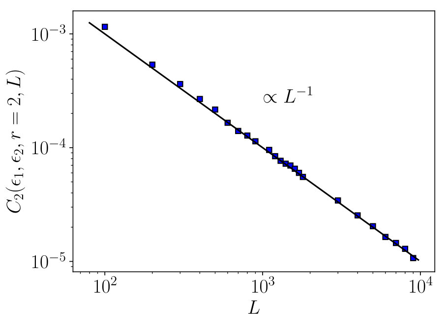 Figure 1
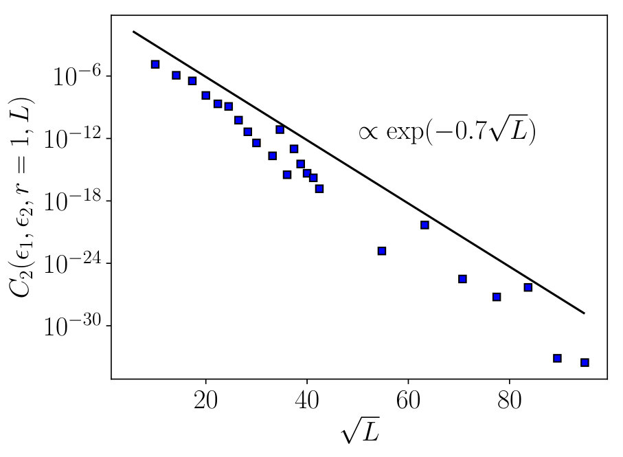 Figure 2
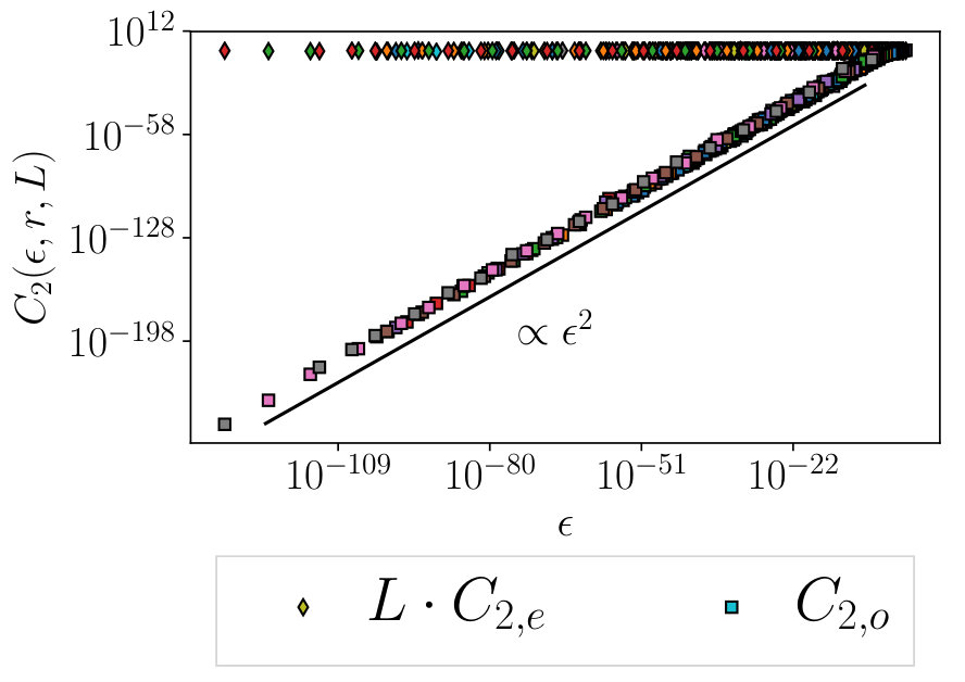 Figure 3
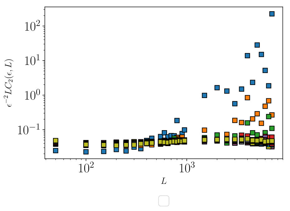 Figure 4
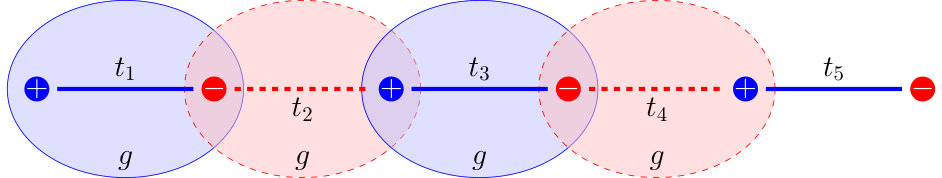 Figure 5
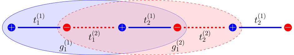 Figure 6
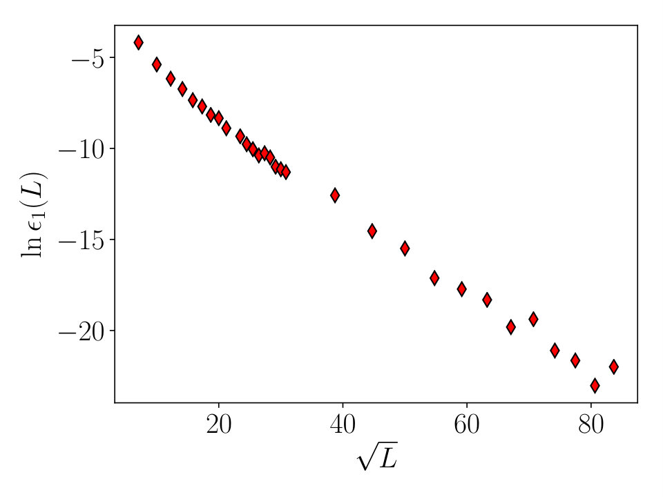 Figure 7
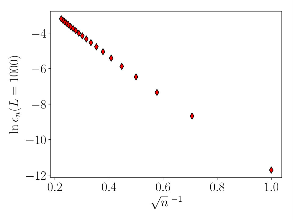 Figure 8
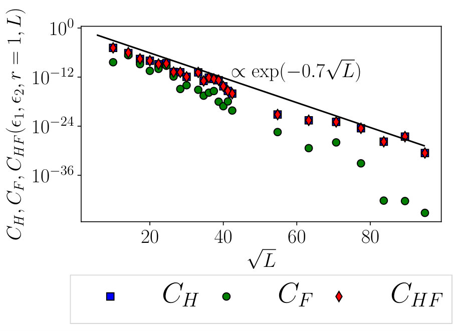 Figure 9
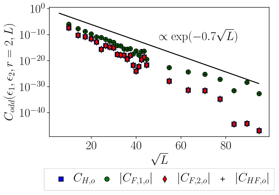 Figure 10
 Figure 11
 Figure 12
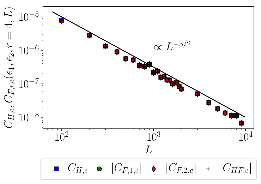 Figure 13
 Figure 14
 Figure 15
 Figure 16
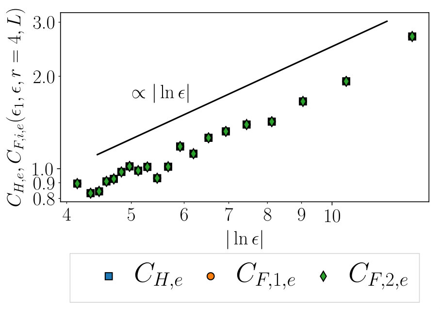 Figure 17
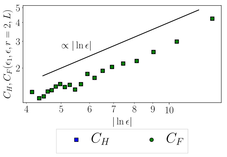 Figure 18
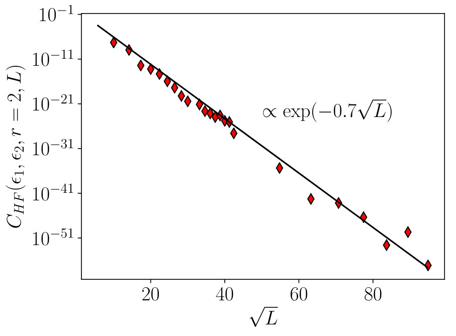 Figure 19
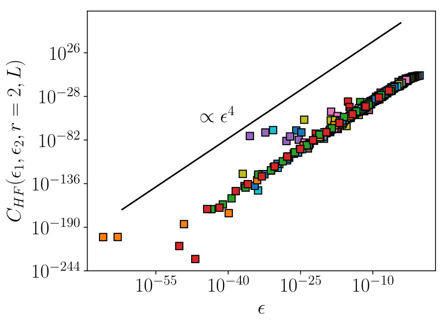 Figure 20
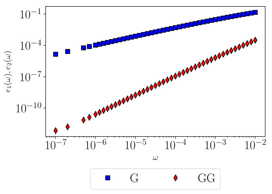 Figure 21
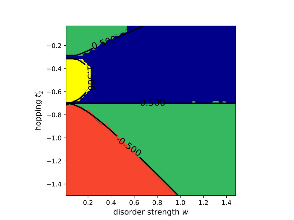 Figure 22
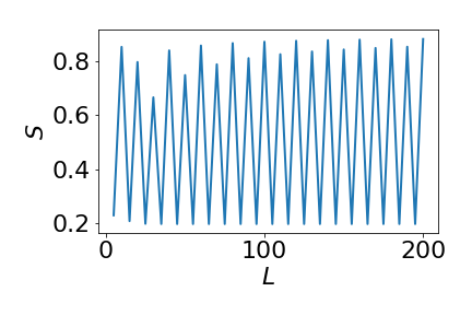 Figure 23
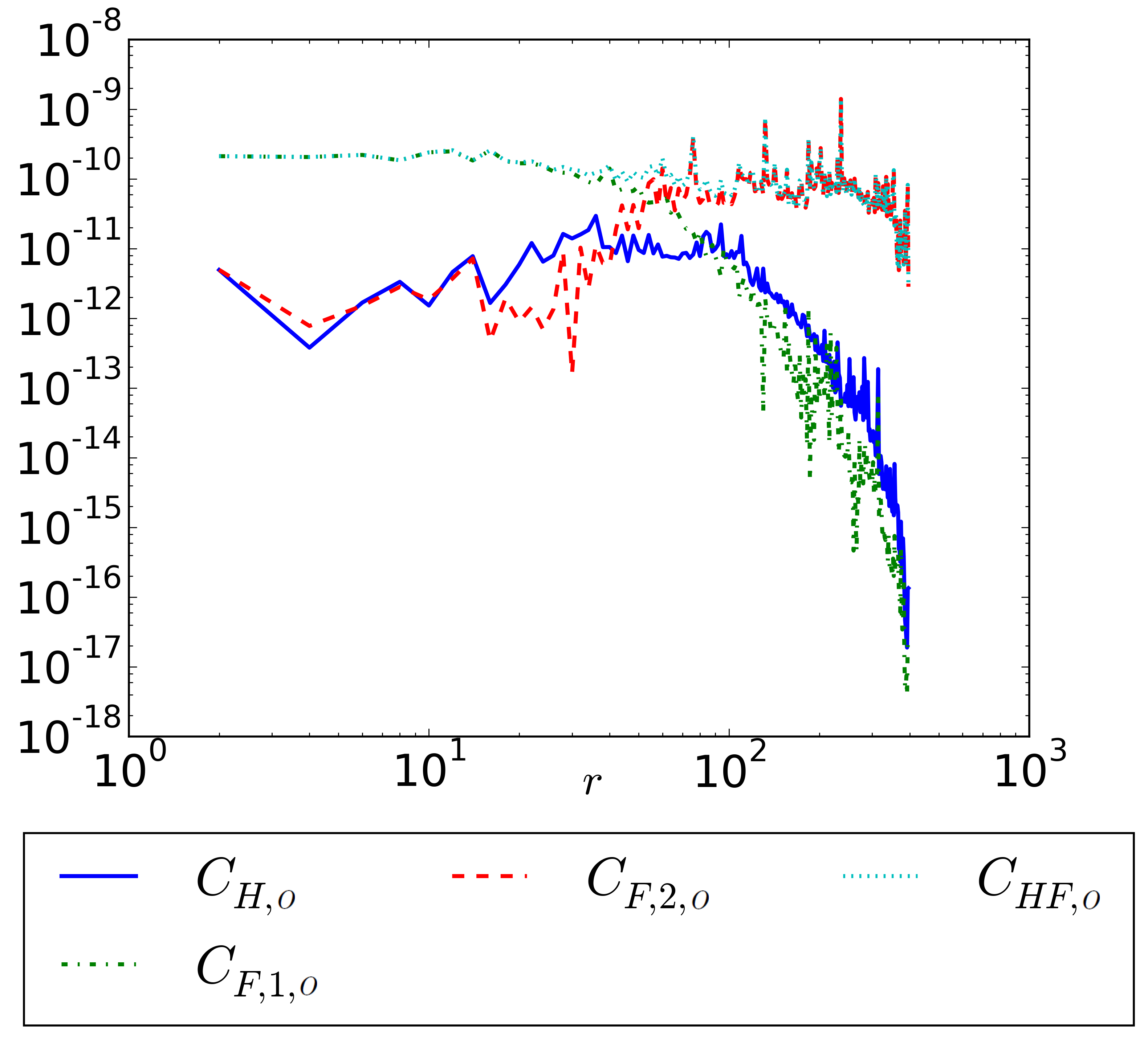 Figure 24
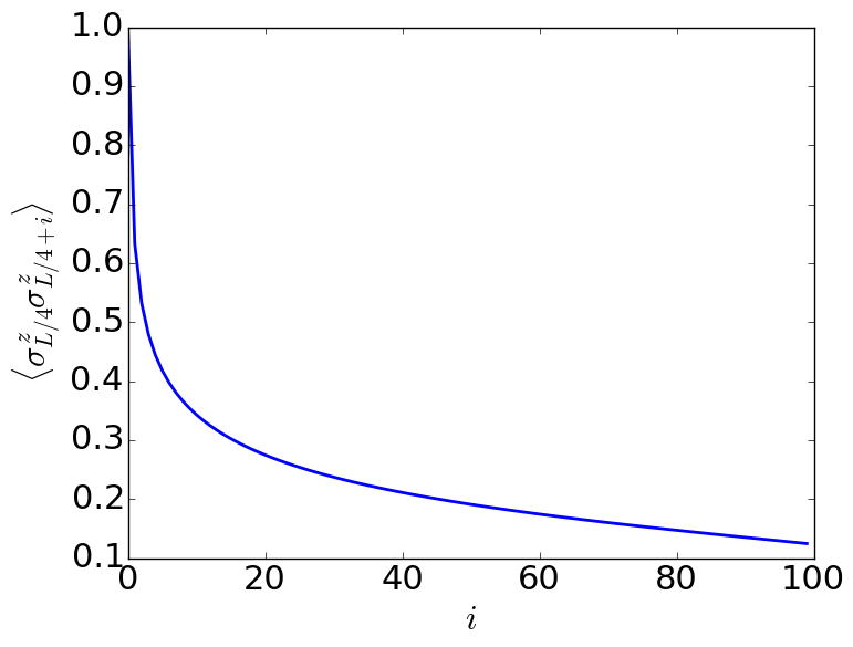 Figure 25
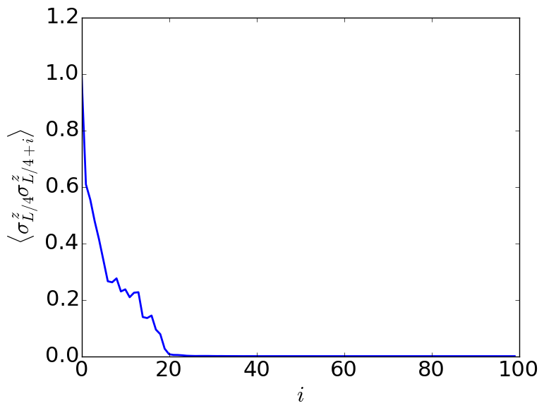 Figure 26
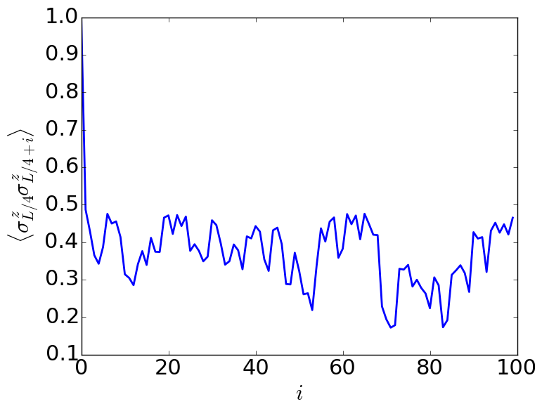 Figure 27
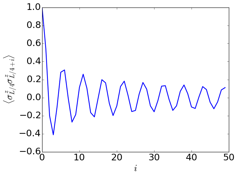 Figure 28
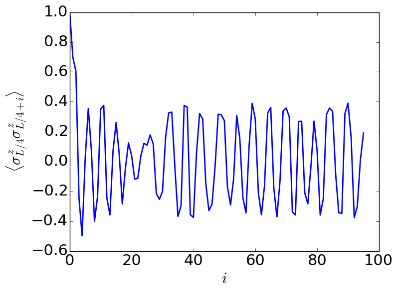 Figure 29
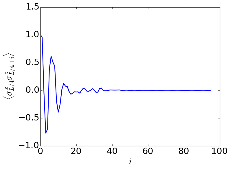 Figure 30
 Figure 31
 Figure 32
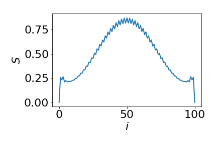 Figure 33
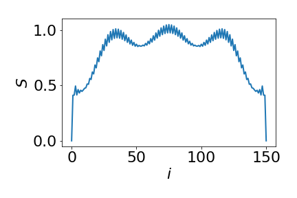 Figure 34
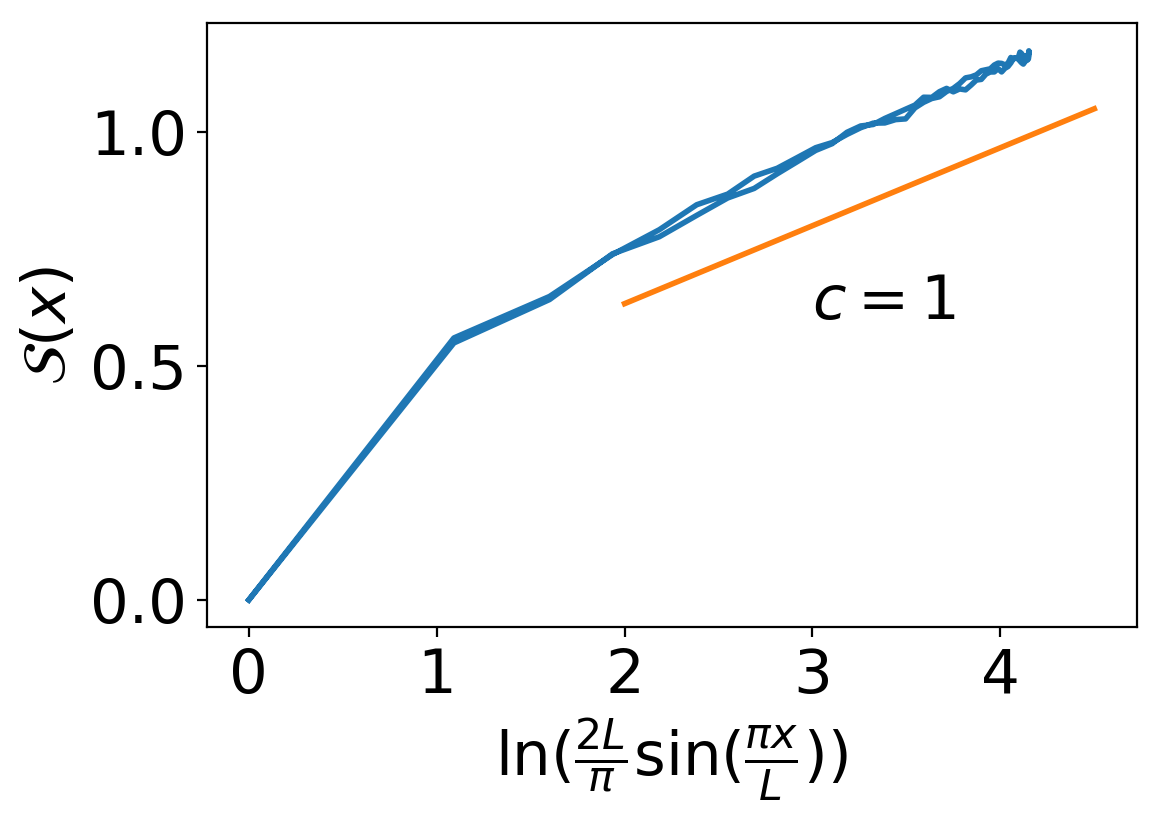 Figure 35
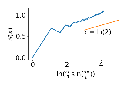 Figure 36
 Figure 37
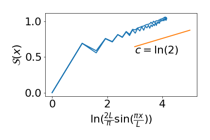 Figure 38
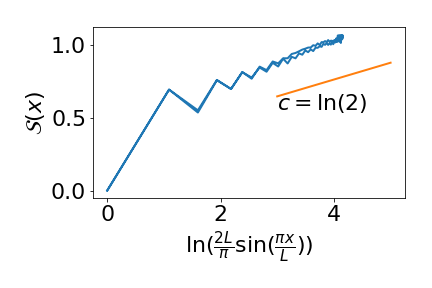 Figure 39
 Figure 40
| coupling | dimension | relevant in |
|---|---|---|
Peer Reviews
No public reviews on file for this paper yet. If you reviewed it on a platform where reviews are public (OpenReview, ICLR, NeurIPS, ICML), you can paste yours below so the community can read it here.
Videos
No videos yet. Explain this paper in a talk, walkthrough, or lecture? Add one.
††thanks: These authors contributed equally to this article††thanks: These authors contributed equally to this article
Disorder and interaction in chiral chains: Majoranas vs complex fermions
J. F. Karcher
Institut für Nanotechnologie, Karlsruhe Institute of Technology, 76021 Karlsruhe, Germany
Institut für Theorie der Kondensierten Materie, Karlsruhe Institute of Technology, 76128 Karlsruhe, Germany
M. Sonner
Institut für Nanotechnologie, Karlsruhe Institute of Technology, 76021 Karlsruhe, Germany
Institut für Theorie der Kondensierten Materie, Karlsruhe Institute of Technology, 76128 Karlsruhe, Germany
A. D. Mirlin
Institut für Nanotechnologie, Karlsruhe Institute of Technology, 76021 Karlsruhe, Germany
Institut für Theorie der Kondensierten Materie, Karlsruhe Institute of Technology, 76128 Karlsruhe, Germany
L. D. Landau Institute for Theoretical Physics RAS, 119334 Moscow, Russia
Petersburg Nuclear Physics Institute,188300 St. Petersburg, Russia.
Abstract
We study the low-energy physics of a chain of Majorana fermions in the presence of interaction and disorder, emphasizing the difference between Majoranas and conventional (complex) fermions. While in the non-interacting limit both models are equivalent (in particular, belong to the same symmetry class BDI and flow towards the same infinite-randomness critical fixed point), their behavior differs drastically once interaction is added. Our density-matrix renormalization group calculations show that the complex-fermion chain remains at the non-interacting fixed point. On the other hand, the Majorana fermion chain experiences a spontaneous symmetry breaking and localizes for repulsive interaction. To explain the instability of the critical Majorana chain with respect to a combined effect of interaction and disorder, we consider interaction as perturbation to the infinite-randomness fixed point and calculate numerically two-wavefunction correlation functions that enter interaction matrix elements. The numerical results supported by analytical arguments exhibit a rich structure of critical eigenstate correlations. This allows us to identify a relevant interaction operator that drives the Majorana chain away from the infinite randomness fixed point. For the case of complex fermions, the interaction is irrelevant.
I Introduction
Topological states of matter represent one of the central directions of the contemporary condensed matter physics Haldane (2017). Systems with topological order are usually characterized by a gap in the bulk and “metallic” states at the boundaries. These boundary states are robust against disorder-induced Anderson localization as long as the disorder is not strong enough to close the gap in the bulkNomura et al. (2007); Moore (2010); Ostrovsky et al. (2007); Ryu et al. (2007).
One-dimensional (1D) systems with topological phases are considered a potential platform for quantum computingSarma et al. (2015); Alicea (2012); Leijnse and Flensberg (2012); Beenakker (2013), as the quantum state is stored non-locally and cannot be destroyed by local, uncorrelated noise (as long as the noise is not strong enough to close the bulk gap). For non-interacting systems, the symmetry classification by Altland and Zirnbauer Altland and Merkt (2001) combined with the analysis of topologies Kitaev (2009); Schnyder et al. (2008); Ryu et al. (2010); Mirlin et al. (2010), extended also to various spatial symmetries Fu and Kane (2007); Fu (2011), has provided a systematic picture of possible topological states. Despite the progress on extending this classification to include weak interactions Fidkowski and Kitaev (2011, 2010); Morimoto et al. (2015), it is still a formidable task to determine which topological phases are present in a given interacting systems. While non-interacting topological phases are robust against disorder-induced localization, this is not always the case for topological states in interacting systems. In particular, in 2D superconductor systems, the combined effect of disorder and interactions has been shown to break entirely the topological protection Foster and Yuzbashyan (2012); Foster et al. (2014). The underlying mechanism is that disorder renders the interaction relevant in the renormalization-group (RG) sense; see also Refs. Ostrovsky et al., 2010; Burmistrov et al., 2012 for related physics. The fact that the interplay of interaction and disorder may crucially affect the physics has been known for a while Finkel’stein (2010); recent works show that it is also of central importance for topological states of matter.
In this work, we explore the the effect of disorder and interaction on the low energy physics of a chain of Majorana quasiparticles commonly called Kitaev chain Kitaev (2001). Note that usually one studies the gapped Kitaev chain, with zero-dimensional Majorana bound states at its ends. In this paper, we will pay particular attention to the combined effect of disorder and interaction on a gapless Majorana chain representing a one-dimensional wire with counterpropagating Majoarana modes. The most local interaction one can have in this system is a four-point Majorana interaction Rahmani et al. (2015). Disorder is introduced by choosing the hopping parameters from a random distribution. This model could potentially be realized by vortex lattices Chiu et al. (2015a); Pikulin et al. (2015); Chiu et al. (2015b) in a thin film topological superconductor. In general, chains of parafermions such as Majoranas can also be realized in superconductor-ferromagnet structures along quantum spin Hall edges Shivamoggi et al. (2010). Further, the (gapped) Kitaev chain Hamiltonian has been realized as an effective low energy theory in InGaAs nanowires on top of a superconductor in a magnetic field Mourik et al. (2012). A gapless Majorana chain can be realized on the edge of an array of such wires Milsted et al. (2015). Other platforms for generating Majorana chains include chains of magnetic atoms on top of a superconductor Nadj-Perge et al. (2014), as well as cold atoms in optical lattices Bühler et al. (2014). The phase diagram of a clean interacting Kitaev chain was studied in Ref. Rahmani et al., 2015.
We will compare the Majorana model to that of complex fermion hopping on a chain with the chemical potential tuned to zero Fisher (1994); Balents and Fisher (1997). In spin language, this model is equivalent to the random bond XXZ model. In the absence of interaction, both Majorana and complex-fermion models belong to the symmetry class BDI and are largely equivalent. The only difference between them is that in the case of complex fermions each pair of states related through chiral symmetry represent two independent single body states, while in the case of the Majorana chain each pair represents a single state. However, the situation changes dramatically once one adds interaction. In the case of complex fermions, previous work based on real-space RG analysis showed that weak interactions are irrelevant in the RG sense Fisher (1994, 1995) and thus do not change the low energy properties of the system. This system flows into a peculiar critical infinite-randomness fixed point. For the interacting disordered Majorana chain, the behavior turns out to be very different. We show that interaction drives the system away from the infinite randomness fixed point, which leads to localization in the case of (even weak) repulsive interaction. The localization of a disordered Majorana chain with moderately strong repulsive interaction was observed previously in Ref. Milsted et al., 2015. We further explain why the above two similar models behave so drastically different once interaction is added.
The outline of the paper is as follows. We define the models and review previous results in Sec. II. In Sec. III, we present our numerical results obtained with the density matrix renormalization groupWhite (1993) (DMRG) code OSMPS Jaschke et al. (2018). We consider first the clean interacting Majorana chain that we drive out of criticality by staggering in order to explore emerging topological phases. Then we turn to the DMRG study of combined effect of disorder and interaction, both for complex fermions and for Majoranas. In the case of complex fermions, we find that properties of a random chain are not essentially influenced by interaction, in consistency with previous results. On the other hand, we observe that the interacting disordered Majorana chain localizes even for weak repulsive interaction. This localization is accompanied by a spontaneous breaking of symmetry between two topological phases that manifests itself in correlation functions. To shed light on the physical origin of these results, we employ in Sec. IV and V two complementary approaches. Specifically, in Sec. IV we use momentum-space RG methods to investigate the effect of weak disorder on the interacting clean models. We show that disorder in both models is strongly relevant rendering the clean fixed point unstable. We thus turn to the complementary approach in Sec. V, where we start from an exact treatment of disorder (which drives the system into the infinite-randomness fixed point) and consider interaction as perturbation. By combining the RG treatment of interaction with a numerical study of wave-function correlations at the infinite-randomness fixed point, we identify a relevant operator in the case of the Majorana chain. No such operator exists in the case of the complex fermionic chain in view of the cancellation between Hartree and Fock contributions. This explains why the Majorana fermion chain is unstable with respect to weak interaction, while the complex fermion chain is stable.
II Models
In this Section we define two 1D models to be considered in this paper: that of complex fermions, Sec. II.1, and of Majoranas, Sec. II.2. We also briefly review some previous results relevant to this work.
II.1 Complex Fermion chain
We start with a spinless fermionic chain where the chemical potential is tuned to zero,
[TABLE]
Every hopping term is between an even (e) and an odd (o) site. The Hamiltonian possesses therefore a sublattice symmetry which is represented by the operator , where is the Pauli matrix operating on the even-odd subspace. By using the local gauge freedom, we can always choose the hopping matrix elements to be real. This implies a time reversal symmetry represented by complex conjugation with . Further, the system possesses in addition the particle hole symmetry expressed by , with . These symmetries place the model in the BDI symmetry class.
We introduce disorder by making the hopping matrix elements random. This does not change the symmetry classification. The most local interaction that can be added to this model is a two-point nearest-neighbor density-density interaction. To keep the system at half filling, a chemical potential proportional to the interaction strength has to be included. Since we will later see that the sublattice structure of the interaction is important, we generalize the interaction to act on sites separated by a distance :
[TABLE]
The couplings of this model for are sketched in Fig. 1.
II.1.1 Spin representation
Using the Jordan-Wigner transformation, one can map the model (2) onto a random-bond, spin- XXZ chain:
[TABLE]
The gauge freedom in the fermionic model corresponds to the spin-rotation symmetry in the plane. While the two models (2) and (4) are equivalent, the Jordan-Wigner transformation is non-local, and so is the mapping between the correlation functions. The spin representation turns out to be particularly suitable for the DMRG analysis and will be used in this paper.
II.1.2 Symmetries and topology
To show that our interaction does not change the symmetry class, we consider the many body generalizations of the above symmetries , see Ref. Chiu et al., 2016. They can be obtained by defining the action of the symmetry operators on the creation and annihilation operators:
[TABLE]
This defines the action of on all operators and states in the Fock space. In this many-body formulation, the time-reversal symmetry and chiral symmetry are represented by anti-unitary operators, while the particle hole symmetry is represented by a unitary operator. In contrast to the single body symmetry operators and , the many body symmetry operators all commute with the Hamiltonian.
Let us now analyze the symmetries of the Hamiltonian (2). First, all couplings are real, implying that commutes with . Second, the term in Eq. (3), which corresponds to a proper choice of the chemical potential ensures that the model is invariant under . Further, the operators and square to unity. The interacting model belongs therefore to the symmetry class BDI. It was shown that 1D interacting systems of complex fermions belonging to this symmetry class (in absence of pairing terms) have a topological invariant Morimoto et al. (2015).
II.1.3 Clean limit
Let us briefly discuss the clean limit. If all matrix elements are equal, , and the interaction is not too strong, the low-energy theory of the XXZ model (4) is the Luttinger liquid. This is a conformal field theory with central charge . For the case of nearest-neighbor interaction, , the corresponding condition isLuther and Peschel (1975) . For the system is gapped.
One can drive the system away from the critical line by introducing a staggering, and , with . This will in general open a gap. More precisely, investigating the RG relevance of the corresponding term in the bosonization language (see analysis in Sec. IV below), we find that the staggering immediately opens a gap for , i.e., almost in the whole range of corresponding to a critical theory. The gapped phases with and are topologically distinct. This can be easily seen by observing that in the limit , the fermion at the first site decouples from the rest of the chain, thus representing a topological zero mode. This zero mode will persist for (although it will spread over a few sites). In the opposite case, , there is no zero mode. The critical theory (Luttinger liquid) thus represents a boundary between two topologically distinct phases.
II.1.4 Noninteracting limit
Consider now a non-interacting system () but in the presence of disorder, i.e. with random hopping matrix elements . This breaks translational symmetry for a given realization of disorder. However, if the distributions of even and odd matrix elements are the same, the system remains self-dual with respect to the transformation . In spin language, the model corresponds to a disordered XY chain. Analytically, the problem can be treated with a real space RG procedure Fisher (1994). At the self-dual point, the system is critical despite an RG flow towards strong disorder. This very peculiar fixed point is termed infinite-randomness fixed point. By considering the scaling of the disorder-averaged entanglement entropy, one can define an effective central charge characterizing this critical state Refael and Moore (2004, 2009); Laflorencie (2005) .
II.2 Majoranas
To introduce the second model—the one that is which is of the central interest for this work—we start with a 1D chain of spinless fermions of length with superconducting pairing matrix elements , hopping and local chemical potential . The pairing and hopping are chosen to be real. The Hamiltonian reads
[TABLE]
Now we rewrite each pair of fermionic creation and annihilation operators in terms of two Hermitian Majorana operators :
[TABLE]
The Majorana operators obey the commutation relations
[TABLE]
Each Majorana operator represents half a degree of freedom. The Hamiltonian becomes now
[TABLE]
If the hopping and pairing terms are chosen such that , this simplifies to
[TABLE]
where we have introduced notations and . This model is known as Kitaev chainKitaev (2001).
We now inspect the symmetries of the non-interacting Hamiltonian (8). The pairing terms in Hamiltonian (8) break the global symmetry to the parity . As usual for Bogolyubov-de Gennes models, the Hamiltonian has a particle hole symmetry . Since we chose all couplings real, the system has time reversal symmetry . Both symmetry operators square to unity, thus the model belongs to class BDI. The product of those two symmetries yields the sublattice symmetry .
Now we include the interaction term. Since , the most local interaction term couples four neighboring Majoranas Rahmani et al. (2015):
[TABLE]
Below we will allow for randomness in the hopping matrix elements . If the values of the interaction as well as the distribution of hopping matrix elements is the same for even and odd sites, the model is self-dual under translation by one side.
II.2.1 Symmetry and topology
The symmetries and can be extended to the many-body setting in analogy with discussion in Sec. II.1.2 for the case of complex fermions. In terms of Majorana operators the symmetries read
[TABLE]
It is worth mentioning that for Bogolyubov-de Gennes Hamiltonians the particle-hole symmetry is not a true many-body symmetry but rather a constraint related to the Fermi statistics, see discussion in Ref. Kennedy and Zirnbauer, 2016. This puts our model in interacting symmetry-class BDI with topological classification, see Ref. Fidkowski and Kitaev, 2011.
While the Hamiltonian (13) contains only nearest-neighbor Majorana hopping , any odd-range hopping is in principle permitted by symmetry. In particular, as we discuss below, the interaction generates third nearest neighbor hopping on the mean-field level. An even-range hopping would couple Majoranas from the same sublattice and break the chiral symmetry and the time-reversal symmetry. Similarly, any interaction term containing an even number of Majorana operators belonging to even sites (and thus an even number of operators from odd sites), is consistent with the and chiral symmetries.
II.2.2 Spin representation
The interacting Kitaev chain (13) can be mapped onto a spin--chain by means of Jordan-Wigner transformation:
[TABLE]
Here and correspond respectively to odd () and even () hopping matrix elements of Eq. (13), and similarly for the interaction couplings . The couplings of this model are sketched in Fig. 2.
It is interesting to note that the odd couplings and couple in the spin language to components, and the the odd couplings and to components. Translation by one site (even-odd transformation) exchanges and . Models related by this transformation are dual, although this duality is less obvious in the spin representation than in the Majorana representation.
We will use the spin representation for the DMRG analysis below.
II.2.3 Noninteracting limit
In the non-interacting limit () the Hamiltonian (17) describes the transverse Ising model. In the clean translational-invariant case (no staggering, ) the system is critical with a 1D Majorana low-energy theory and central charge . In the presence of random hopping, the model is at the infinite-randomness fixed point Fisher (1995) as noted above in the context of complex fermions in Sec. II.1.4. The difference between the two models in the absence of interaction is that two single-particle states of the complex-fermion model correspond to a single state of the Majorana model. As a consequence, the effective central charge at the infinite-randomness fixed point is halved, .
II.2.4 Clean limit
For the case of interacting model with homogenous couplings, and , Rahmani et al. Rahmani et al. (2015) have determined the phase diagram:
- •
Strong interaction. The system is gapped for very strong interactions of both signs ( or ). The translation symmetry gets spontaneously broken, and the transition between the topologically distinct phases is of first order type.
- •
Attractive interaction. There is a critical phase up to very strong interactions . The low energy theory is a single Majorana mode with central charge . This phase is controlled by the same fixed point as the transverse Ising model and therefore dubbed Ising phase.
- •
Weak repulsive interaction. For the case of repulsive interaction (), the Ising phase is stable for sufficiently weak interactions, .
- •
Intermediate repulsive interaction. For repulsive interaction of intermediate strength, , a phase emerges with coexisting Luttinger-liquid and Majorana modes. Alternatively, one can say that a single Majorana mode of the non-interacting theory is promoted to three Majorana modes, which can be understood already by mean-field level treatment of the interaction. The central charges in this phase is .
III DMRG results
It is viable to calculate the groundstate properties of systems with length of the order of a few hundred sites using methods based on matrix-product states (MPS). For these methods, spin models are most convenient. All DMRG calculations in this work have therefore been done on the spin representations, Eq. (4) and Eq. (17), using the software OSMPS Jaschke et al. (2018). The maximum bond dimension was chosen to be 512, states with weight smaller than were truncated.
III.1 Interacting Majorana chain with staggering
As we will later see, disorder drives an interacting Majorana chain into different localized phases if the interaction is repulsive. To obtain an overview over possible localized phases in the Majorana model, we first consider the clean model and drive the system out of criticality by introducing staggering. We calculate the ground state of the clean Majorana chain, Eq. (17) with , , , and , and spin sites (which corresponds to Majorana sites). We choose parameters in such a way that the relation is maintained; we use a short-hand notation for this ratio. By using DMRG, we explore the range of the interaction strength, varying the staggering, . For the staggering region , the hopping is fixed and is varied, while for staggering above the self-dual line , is fixed and is varied.
The system with a given value of staggering is related to the system with inverse staggering via duality transformation. In the Majorana representation, this transformation corresponds simply to a translation by one lattice site. On the other hand, in the spin language of Eq. (17) the duality transformation is much less trivial (and, in particular, non-local).
In the MPS representation the (von Neumann) entanglement entropy between two subsystems split by a bond is readily available Schollwoeck (2011); Jaschke et al. (2018). In a critical 1D system of length with open boundary conditions, the bond entropy scales as a function of bond position as Bazavov et al. (2017)
[TABLE]
where is the central charge and the topological entanglement entropy. The slope of the dependence of the entanglement entropy on the scaling function entering Eq. (18) can thus be used to extract the central charge of the system. In gapped systems, the entanglement entropy saturates, i.e., .
In order to identify critical lines and regions, the central charge defined according to Eq. (18) is plotted in Fig. 3 via a color map in the parameter plane spanned by the interaction strength and the staggering . Further, we show in a similar way in Fig. 4 the long-range spin-spin correlation . This plot helps to differentiate between topologically distinct gapped regions. Figure 5 provides an overview over our results that are discussed in more detail below. In this figure, numbers from 1 to 6 label different regions; the corresponding distance dependences of spin correlations is shown (with the same labels) in Fig. 6. On the self-dual line, , the range of interaction strength can be divided, in agreement with Ref. Rahmani et al., 2015, into three intervals: the Ising phase for attractive and relatively weak repulsive interaction, , the phase where the Ising sector coexists with a Luttinger liquid sector for repulsive interaction in the interval , and a gapped phase for even stronger repulsive interaction, . This distinction remains useful also for understanding of phases in the presence of staggering, as discussed below.
III.1.1 Attractive and weak repulsive interaction
In the absence of staggering, , the system remains in the non-interacting Ising phase for attractive interaction and for repulsive interaction, , as was found in Ref. Rahmani et al., 2015. Indeed, we observe in Fig. 3 that on the self-dual line the system is critical with a central charge of at this range of interactions. At finite staggering the system is gapped, with two topologically distinct phases (labeled 2 and 3 in Fig. 5) that can be distinguished by the behavior of the spin-spin correlator. For staggering , which corresponds to the topologically trivial phase in the fermionic picture, it decays quickly with distance, see Fig. 4 and the top left panel of Fig. 6. On the other hand, in the symmetry-broken phase in the spin language, (which is topologically non-trivial in the fermion language), the correlator saturates at a constant value of order unity at large distance, Fig. 4 and the bottom left panel of Fig. 6. On the critical line , the correlator decays slowly (algebraically), as expected, see middle left panel of Fig. 6.
III.1.2 Intermediate repulsive interaction
For stronger repulsive interaction , the clean system without staggering exhibits a Luttinger liquid sector in addition to the Ising sector as has been already pointed out in Sec. II.2.4. In this paper we will call this phase “Ising + LL” phase, where “LL” stands for “Luttinger liquid”. In Ref. Rahmani et al., 2015 this phase is called the “floating” phase, in analogy to a similar phase in the anisotropic next nearest neighbor Ising model. It is characterized by a central charge of . Our numerical data in Fig. 3 confirm this behavior.
As Fig. 3 demonstrates, the staggering does not immediately lead to a gapped system in this interaction range. Instead, there is an extended region of finite staggering with a central charge of around the no-staggering line. This can be understood as a result of the Luttinger-liquid sector being stable to weak staggering, with the Ising sector becoming gapped. An argument based on RG analysis is given in Sec. IV. More precisely, there are two such phases with , labeled 5 and 6 in Fig. 5, which are separated by the line with (label 4).
In these extended critical regions, the spin-spin correlator is an oscillating function of distance, as detailed in Fig. 6. The oscillation decay above the no-staggering line (label 6, top right panel), while their amplitude remains constant below this line (label 5, bottom right panel). On the line without staggering, the oscillations decay very slowly (label 4, middle right panel). The non-decaying oscillation in the extended critical region below the self-dual line are also visible in Fig. 4.
At extreme staggering , the model reduces to the longitudinal Ising model. This model exhibits a first order transition at the point . The critical region with central charge is separated from the gapped region of the Ising phase by a line connecting this point ( and ; marked by a black dot in Fig. 5) with the point of the Lifshitz transition on the critical line ( and ; marked by a red star in Fig. 5). Additionally, there is a vertical critical line (red) connecting the black dot to its dual. This line is also clearly visible in the picture of the central charge, Fig. 3, as it has a central charge of .
At variance with the horizontal line that is determined by the condition of no staggering, the vertical line is not fixed by any simple symmetry. We have thus performed additional checks to verify its position. First, in order to exclude finite-size effects, we have considered twice larger systems () in this part of the phase diagram. The results demonstrated that neither the obtained value nor the position of the line change with . This implies that the vertical line is indeed a property of the system in the thermodynamic limit. Second, we have looked more carefully at the precise location of the line and found that it is not exactly at , although very close to it. As an example, we find that the line crosses the horizontal line at . This indicates that the “vertical” line is not exactly straight but rather shows a small deviation from the line .
Analogous to the horizontal (no-staggering) critical line, the value can be understood as a superposition of a Luttinger liquid () and a Majorana mode () due to a topological phase boundary.
To shed light on the reason for the emergence of the vertical line, we have performed a mean-field analysis by generalizing that of Ref. Sen and Chakrabarti, 1991 to our problem. In this way, we have approximately mapped an interacting fermionic Hamiltonian to a non-interacting (mean-field) one and obtained the condition for gap closing. This condition yields a two-dimensional surface in the whole (three-dimensional) space of parameters (, , and ). The surface can be computed numerically. We observe numerically that this two-dimensional surface intersects the two-dimensional surface determined by the condition (that is used in our DMRG numerics) on two lines – the horizontal and the vertical ones. The numerically obtained position of the vertical line is close to . With the superimposed extended Luttinger liquid phase, we have on these lines. In analogy with the horizontal line, the vertical line corresponds to the gap closing in the Ising sector, which corresponds to a phase boundary between topologically distinct phases.
Another interesting point is the red patch appearing in the upper plane seemingly violating the duality of the model. This is more than a numerical artifact and has to do with corrections to the scaling form of the entanglement entropy (18) in gapped phases. We refer to Appendix E for a more detailed discussion.
III.1.3 Strong repulsive interaction
With increasing strength of repulsive interaction , the extended critical region around the no-staggering line gradually shrinks, see Fig. 3. For sufficiently strong interaction this region vanishes and, moreover, the line of no-staggering becomes gapped.
III.2 Interacting Majorana chain with disorder
We now introduce disorder in the interacting Majorana chain model by choosing hopping as random independent variables, with a homogeneous distribution over the interval . All hopping matrix elements have now the same distribution, so that there is no staggering.
In general, critical lines can move in phase space as function of disorder strength Gergs et al. (2016); McGinley et al. (2017). However, the critical line at no staggering is pinned by self-duality. Therefore, it should remain critical in the presence of both disorder and interaction unless spontaneous symmetry breaking takes place, see a more detailed discussion in Sec. III.2.2 below.
Since the average value of the hopping matrix elements is unity, the value of the interaction has now the same meaning as in the analysis of the clean system. We consider three different ranges of interaction strength: (i) attractive interaction , (ii) weak repulsive interaction and (iii) medium repulsive interaction . We calculate the effective central charge in these regions of interaction by analyzing the disorder-averaged entanglement entropy via Eq. (18).
III.2.1 Attractive interaction
For attractive interaction , the clean system is in the Ising phaseRahmani et al. (2015) with a central charge of , see Sec. III.1.1 and left panel of Fig. 7. On the other hand, the disordered non-interacting system has an effective central charge of as was found in Ref. Refael and Moore, 2009. Our numerics confirms this value.
Remarkably, in the presence of both disorder and interaction, the central charge returns to the value of the clean system , see Fig. 7 (right panel). For higher attractive interaction, the disorder averaging requires less samples in order to give a smooth function of the entanglement entropy vs scaling function than for lower interaction. This serves as an additional indication that disorder does not play an important role for the Majorana chain with attractive interaction.
III.2.2 Weak repulsive interaction
The clean system stays critical with for weak repulsive interaction Rahmani et al. (2015), , see Sec. III.1.1 and the left panel of Fig. 8. We find that adding disorder leads to localization, see right panel of Fig. 8. This appears to happen for arbitrarily weak repulsive interaction and arbitrarily weak disorder. Due to duality, the critical lines have to be mirror symmetric around the self-dual line with respect to staggering. This holds also when the system is disordered. For this reason, the critical line cannot simply bend away from the self dual line. If the system localizes on the self-dual line, there are therefore two possibilities: (i) the critical line splits up into two lines with equal central charge, leaving a gapped region around the self-dual line, or (ii) the critical line terminates, and the transition between the region above and below the self-dual line becomes first order. It is shown in Appendix C by treating the interaction at the mean-field level that the criticality is pinned to the self-dual line for all interaction values and disorder strengths. This excludes the option (i), thus implying that the possibility (ii) is realized.
We thus conclude that, for a disordered system with repulsive interaction, the symmetry gets spontaneously broken, and the system undergoes a first-order transition on the self-dual line. This is also reflected in the distance dependence of the spin correlation function. Specifically, we find that, depending on the disorder configuration, this correlation function shows one of two types of behavior: it either very quickly decays to zero or fluctuates around a value of order unity. This is illustrated in Fig. 9 where the results for two disorder configurations are shown. These two types of behavior correspond to two topologically distinct phases, as is clear from the comparison of two panels of Fig. 9 with the top left and bottom left panels of Fig. 6. In the latter figure, the topologically distinct phases were induced by staggering (in a clean model) breaking explicitly the symmetry with respect to the duality transformation. We now see that adding disorder breaks spontaneously the symmetry of the system on the no-staggering line, placing it into one of the two topologically distinct phases. The transition between these two topological phases becomes thus first order.
III.2.3 Medium repulsive interaction
If the repulsive interaction is in the interval the clean system is in the Ising+LLRahmani et al. (2015) phase which is characterized by a central charge of , see Sec. III.1.2 and left panel of Fig. 10. Our results show that, similar to the case of weak repulsive interaction, disorder leads to localized behavior also in this range of interaction, see right panel of Fig. 10. This was also found in Ref. Milsted et al., 2015.
As in the case of weak repulsive interaction, the spontaneous symmetry breaking by disorder can be visualized by inspecting the spin-spin correlation function for individual realizations of disorder. We find again two distinct types of behavior that are illustrated in Fig. 11: oscillations without decay or with a quick decay. The behavior shown in the left panel of Fig. 11 corresponds to that in the clean model in the Ising+LL phase with staggering , see bottom right panel of Fig. 6, while the behavior shown in the right panel of Fig. 11 corresponds to that in the clean model with staggering , see top right panel of Fig. 6. Thus, the symmetry between the two topological phases gets broken spontaneously by disorder in full analogy with the weak-repulsion regime. A comparison of Figs. 9 and 11 reveals an interesting difference between the weak-repulsion and intermediate-repulsion topological phases. Specifically, in the latter case the correlator shows oscillations around zero, thus changing sign.
III.3 Disordered Fermionic chain
We turn now to the DMRG results for a disordered interacting fermionic chain, Eq. (2). The results for the entanglement entropy are shown in Fig. 12 for the cases of odd () and even () interaction distances. We observe that the (sufficiently weak) interaction does not modify the behavior of the disordered system: both for and the interacting system remains critical and has the central charge characteristic for the infinite-randomness fixed point. This implies the RG-irrelevance of the interaction.
IV Renormalization group around the clean fixed point
Numerical results of Sec. III.2 for a disordered interacting Majorana chain indicate that in the presence of disorder an interaction of either sign becomes relevant. To get the corresponding analytical insight, one has to consider a model with both interaction and disorder, which is an extremely challenging problem. In this Section we approach this problem by starting from a clean interacting Majorana chain and exploring the effect of weak disorder.
The stability of the clean fixed points of the interacting fermionic and Majorana models can be probed by a weak-disorder momentum-space RG analysis. For this purpose, we consider the low-energy theory in the continuum limit. In the case of the complex fermionic chain, this is a Luttinger liquid (LL) theory. In the Majorana case, it is either a Majorana theory (, Ising phase) or a Majorana theory with an additional LL sector (, Ising +LL phase), depending on the interaction strength. The density-density parts of the interaction are quadratic in Luttinger theory and renormalize the Luttinger parameter .
In these continuum theories, disorder appears as a random-mass term. Choosing nonzero average of the mass or a constant non-vanishing mass corresponds to staggering. By including such terms, one can draw conclusions about the stability with respect to staggering, which is another goal of the present section. This should help understanding the appearance of extended gapless phases that were found by DMRG numerical analysis in Sec. III.1.
We will show below that at any of the fixed points of the clean Majorana chain (Ising or Ising + LL), the disorder becomes relevant and flows to the strong-coupling regime. This happens also for the complex-fermion fixed point (Luttinger liquid) if the interaction is not too strong. This will lead us to the complementary analysis in Sec. V, where we treat disorder exactly and the interaction as a perturbation.
IV.1 Majorana: fixed point
The continuum decomposition in slow modes of the lattice Majorana operators is
[TABLE]
For a Majorana low energy theory disorder corresponds to a random-mass term of the form:
[TABLE]
A constant mass corresponds to a staggering; it directly opens a gap of size .
The disorder is assumed to be Gaussian white noise with ; one can also include a staggering by introducing a non-zero mean . Treating the disorder by using the replica trick, one straightforwardly finds that the term generated by disorder has (upon disorder averaging) the scaling dimension and is therefore relevant in the RG sense. This term drives the system away from the clean fixed point. However, this does not necessarily mean that the system becomes gapped. For example, in the non-interacting case (and in the absence of staggering) the system flows to the critical infinite-randomness fixed point Fisher (1995). It means, however, that an analysis based on RG around the clean fixed point is insufficient to understand the infrared physics of the problem and suggests a complementary approach as implemented in Sec. V.
Finally it should be noted that no relevant interaction term can be written down in a Majorana low-energy theory. Indeed, the interaction should involve at least four Majorana operators with scaling dimension each and two derivatives with dimension . The most relevant term thus has scaling dimension and is strongly irrelevant.
IV.2 Complex fermions: Luttinger liquid () fixed point
Lattice operators are related to their continuum versions as follows
[TABLE]
In the presence of interaction , bosonization has to be employed. Here the following conventions relating the fermionic fields to the bosonic fields are used:
[TABLE]
The Klein factors are not important in any of the following considerations.
The exact dependence of the Luttinger parameter on the parameters of the lattice model is knownLuther and Peschel (1975):
[TABLE]
Disorder and staggering introduce a mass term of the form:
[TABLE]
The scaling dimension of a constant mass term is . This means that it is relevant for , which corresponds, in terms of the microscopic parameters, to the interval covering almost the whole range of critical theories, .
The scaling dimension of the quartic term generated by disorder, as obtained by
the replica field-theory approach, is . It depends thus on the Luttinger parameter
whether the disorder is relevant or not. Specifically, for the disorder is relevant, while for the model remains at the clean fixed point in the presence of weak disorder. We have checked the latter prediction by DMRG, see Fig. 13 for the scaling of the entanglement entropy at strong attractive interaction, , and sufficiently weak disorder. We find , as expected for the system at the Luttinger-liquid fixed point.
Around the non-interacting limit, i.e. for sufficiently close to unity, the disorder is strongly relevant, as expected.
We also briefly discuss allowed interaction terms as perturbations to the Luttinger liquid fixed point. They are of three types. First, the density-density interaction is marginal and simply modifies the value of . Second, terms that are of higher order in or contain gradients are strongly irrelevant. Finally, the staggering yields sine and cosine terms that are relevant in a range of (in particular, around the weak-interaction point ). On the self-dual line, these latter terms are absent.
IV.3 Majorana chain: Ising+Luttinger liquid () fixed point
We turn now to the fixed point of the clean Majorana chain that emerges in a range of medium-strength repulsive interactions, as discussed above. It was suggested in Ref. Rahmani et al., 2015 that, at this fixed point, the low-energy theory consist of Majorana and Luttinger-liquid sectors, see also Sec. II.2.4 and III.1.2. This can be understood by considering the quadratic form of the action including the third-nearest-neighbor hopping which is generated by mean-field treatment of the interaction (or, alternatively, under RG flow):
[TABLE]
The third-nearest-neighbor hopping term modifies the dispersion such that there are now three Majorana modes, or, equivalently, a fermionic mode emerge in addition to the Majorana mode. The lattice Majorana operator then has the following low-energy decomposition Rahmani et al. (2015):
[TABLE]
where is the effective Fermi momentum. The interaction generates now the density-density interaction of the fermions , . To treat this interaction exactly, we employ the bosonization approach. Another interaction term couples the resulting Luttinger liquid to the Majoranas with strength , see Eq. (81).
Next, let us discuss the stability with respect to staggering. The kinetic term has oscillatory components with wave vectors , , , , , and . A constant mass term describing staggering couples to the -component of the kinetic term:
[TABLE]
The Majoranas are then immediately gapped out. On the other hand, the cosine term in the Luttinger-liquid sector is relevant only for . There is therefore a region of the interaction strength where the Luttinger liquid is stable towards staggering. This explains the existence of the extended gapless phase with observed numerically, see Fig. 3 and the schematic phase diagram in Fig. 5.
Now we analyze the effect of disorder that is treated as a weak perturbation. Combining the oscillatory components of the kinetic term (with the six wave vectors listed above) with the corresponding Fourier components of the random mass yields non-oscillatory contributions. We get therefore six independent disorder couplings that coincide at the beginning of the RG flow but renormalize differently. Details on implementation of the RG procedure are presented in Appendix A. In Eq. (80), the disorder-induced terms in the action (with the replica formalism used to average over disorder) are presented. While the forward scattering cannot be gauged away straightforwardly, a more detailed calculation shows that it does not change the results presented here.
In Table 1, we list the scaling dimensions of the disorder couplings resulting from the corresponding RG equations. They determine the range of in which the disorder-induced terms are RG-relevant. We observe that at least one of the couplings is relevant for any value of , i.e. the disorder always drives the system aways from the clean fixed point. In analogy with the conventional Giamarchi-Schulz RG Giamarchi and Schulz (1988), the RG equations for the disorder-induced couplings are complemented by the flow equation for the Luttinger constant :
[TABLE]
Here and are dimensionless coupling constants for the disorder-induced terms with momentum component in terms of lattice spacing and Luttinger-liquid velocity . In Eq. (28), we have kept only the contribution of the couplings and to the renormalization of . In principle, the other couplings also contribute to this renormalization; however, they are less relevant for around unity, so that we have neglected their contributions.
A brief summary of main conclusions that we draw from this RG is as follows. First, the Ising+LL clean fixed point is stable towards interaction. Indeed, this phase is characterized by a repulsive interaction, hence , so that the coupling is irrelevant. In fact, a higher order coupling between the LL and Majorana sectors becomes relevant for very strong interaction Rahmani et al. (2015), , so that the range of stability in the absence of disorder is . Second, over an extended parameter regime, the staggering is irrelevant in agreement with the numerical results of Sec. III.1.2, see Fig. 3. Third, and most importantly, the disorder at the Ising+LL fixed point always runs to strong coupling. In other words, this fixed point is unstable with respect to disorder.
The results obtained in Sec. IV demonstrate that the weak-disorder analysis is not sufficient for Majorana chain, both in the and phases of the clean system. The RG relevance of disorder is also supported by the analysis in Appendix C where the exact treatment of disorder is combined with mean-field treatment of the interaction. The disorder is also RG relevant for the complex-fermion chain if the interaction is not too strong. These results motivate us to perform in Sec. V a complementary analysis. We will start there from an exact treatment of disorder and will include interaction as a weak perturbation.
V Strong randomness fixed point: Eigenfunction statistics and effect of interactions
In Sec. IV, we have seen that the combined effect of interaction and disorder cannot be understood as a perturbation around the clean interacting fixed point. Specifically, we have established that disorder is strongly relevant at the clean fixed point, thus quickly increasing under RG. We know that, in the absence of interaction, this RG flow leads to the critical infinite-randomness fixed point. It is thus a natural question whether this fixed point is stable or not with respect to interaction. This question is addressed in the present section. Our analysis has much in common with the investigation of stability of 2D surface states of disordered topological superconductors with respect to interaction Foster and Yuzbashyan (2012); Foster et al. (2014). A closely related physics controls the enhancement of superconducting and ferromagnetic instabilities by disorder in 2D systems Burmistrov et al. (2012, 2015). Further, there are close connections with the analysis of the anomalous scaling dimension of interaction in context of the study of decoherence and the dynamical critical exponent at the quantum-Hall transition with short-range interactionLee and Wang (1996); Wang et al. (2000); Burmistrov et al. (2011).
In the clean system, the relevance or irrelevance of an operator can be often established by a relatively straightforward power counting. As an example, this was done in Sec. IV to show that interactions are RG-irrelevant at the clean fixed point of the Majorana chain. In the presence of disorder, the situation is much more complex, since the multifractal nature of wavefunctions as well as a non-trivial scaling of the density of states have to be taken into account. Formally, this disorder-induced renormalization of the interaction can be expressed by an RG equation of the form Foster and Yuzbashyan (2012); Foster et al. (2014)
[TABLE]
Here is the scaling dimension of the density of states of a non-interacting system, with and corresponding to the cases of vanishing and diverging density of states, respectively. Further, is the scaling dimension of the four-fermion interaction operator with respect to the non-interacting theory. For a detailed derivation of Eq. (29) we refer the reader to Appendix C of Ref. Foster et al., 2014. If the right-hand side of Eq. (29) is positive, the interaction is relevant at the non-interacting fixed point; otherwise it is irrelevant.
For a short-range interaction, and in the case when cancellations of the Hartree-Fock type (see below) are not operative, the scaling dimension is equal to the dimension of the squared density of states (which is also a local four-fermion operator). For the clean system is simply equal to but for a disordered system one has in general in view of multifractality (characterizing strong fluctuations of the density of states) Evers and Mirlin (2008); Foster et al. (2014); Gruzberg et al. (2013). Specifically,
[TABLE]
where is the anomalous dimension of the fourth moment of the eigenfunction ( in the notations used below). In this situation of the maximally relevant interaction (no suppression due to Hartree-Fock cancellation or other reasons), Eq. (29) takes the form
[TABLE]
The sum of two exponents and in the r.h.s. of Eq. (31) determines the scaling with of the product of the density of states and the Hartree-type correlation function [defined in Eq. (58) below] for .
In general, since the effect of the interaction can be suppressed due to Hartree-Fock-type cancellation. In this generic situation, we have, in analogy with Eq. (30),
[TABLE]
where is the anomalous dimension of the eigenstate correlation function corresponding to the matrix element of the interaction (and thus taking into account possible Hartree-Fock-type cancellations; see, e.g., Eq. (57) for the case of complex fermions below). Substituting Eq. (32) into Eq. (29), we get
[TABLE]
The sum of the exponents and in the r.h.s. of Eq. (33) corresponds to the scaling with of the product of the density of states and the correlation function . Below we determine the explicit form of this correlation function by inspecting the expectation value of the interaction operator and analyze the scaling of the product with for the models of complex fermions (Sec. V.2) and for the Majorana model (Sec. V.3).
If , the interaction is RG-irrelevant, i.e., the non-interacting fixed point is stable with respect to inclusion of not too strong interaction. In the opposite case, , the interaction is RG-relevant and drives the system away from the non-interacting fixed point. It was found in previous works on the effect of interaction at critical points of higher spatial dimensionality (, with a particular focus on 2D systems)Foster and Yuzbashyan (2012); Foster et al. (2014); Ostrovsky et al. (2010); Burmistrov et al. (2012); Lee and Wang (1996); Wang et al. (2000); Burmistrov et al. (2011) that both these scenarios can be realized. Whether the interaction is relevant or irrelevant depends on the specific non-interacting critical theory considered (i.e., spatial dimensionality as well as symmetry and topology class). As we show below, both scenarios are also realized in the context of the present work (1D critical systems of class BDI): the interaction is irrelevant in the case of complex fermions and relevant in the Majorana model.
The present problem has much in common with Anderson-localization critical points studied in previous works where the multifractality induces strong correlations between eigenstates at different spatial points and different energies (often referred to as Chalker scaling). In fact, critical singularities are particularly strong in the present case. In the more conventional situation, both the density of states and the eigenstate correlation function (and, correspondingly, their product) exhibit a power-law scaling with , so that the indices and are constant (i.e., independent on ). On the other hand, we will see below that in the present problem and (in the complex-fermion case) scale exponentially with , which means that and are -dependent and increase (by absolute value) at large as . This is a manifestation of the fact that the 1D critical point studied here is characterized by very strong multifractality. What we are interested in is the sign of at large which controls the behavior (increase or decrease) of in the limit .
For systems of the symmetry class BDI in one dimension with an odd number of channels, the density of states at low energies exhibits the well known Dyson singularityDyson (1953); Balents and Fisher (1997); McKenzie (1996); Titov et al. (2001):
[TABLE]
We can use this result to calculate the position of the n-th level in a system of the length :
[TABLE]
which yields
[TABLE]
We have verified the scaling (36) numerically for the model with the nearest-neighbor hopping matrix elements uniformly distributed over the interval . The numerical data shown in Fig. 14 fully confirm the analytical prediction, with the coefficient . Thus, we can write down the density of states around the lowest energy state as a function of the length :
[TABLE]
This behavior is not of power-law type, i.e., it is not characterized by a critical exponent in the usual sense. We can define, however, an -dependent scaling exponent , with the result
[TABLE]
The result (38) for the scaling dimension of the density of states is valid both for the Majorana and complex fermions, since these models are equivalent in the absence of interaction. (The only difference is that the number of states is halved in the case of Majoranas.) On the other hand, we will show that the scaling dimension of the interaction is completely different in these two models. We will explore the scaling of interaction by a numerical approach, supporting the results by analytical arguments.
V.1 Scaling of interaction
In order to determine the scaling of the interaction operators, we express the interaction matrix elements in terms of linear combinations of products of single-particle eigenfunctions. These expression in terms of the eigenfunctions are then numerically averaged over the disorder. The numerical results will be also supported by analytical considerations (Appendix D).
We start by writing the most general non-interacting Hamiltonian of a 1D system of size of symmetry class BDI Evers and Mirlin (2008):
[TABLE]
where is a real matrix and , are onsite operators acting on the two sublattices. In the case of the complex fermionic chain, these are fermionic creation and annihilation operators, in the case of the Majorana chain we have and , where are the real Majorana operators in Eq. (12). Diagonalizing the matrix in Eq. (44), one can rewrite the Hamiltonian in the basis of operators which correspond to the single particle excitations of the system,
[TABLE]
Here is a diagonal matrix with eigenvalues . In the case of complex fermions, the eigenvectors are just the conventional single-particle wavefunction . The ground state of the Hamiltonian can be written in terms of the operators and the zero-particle state :
[TABLE]
This immediately yields the action of the operators on the ground state:
[TABLE]
A general -body interaction operator can be expressed as sum of products of annihilation and creation operators of the following type:
[TABLE]
The expectation value of the operator over any eigenstate of a non-interacting system can now be calculated by substituting Eq. (51) into Eq.(55):
[TABLE]
The expectation value that stands as a last factor on the right-hand side of Eq. (56) is non-zero only if the states and are pairwise identical; in this case, it is equal to or , depending on parity of the permutation of indices. The right-hand side of Eq. (56) thus represents an algebraic sum of products of single-particle eigenfunctions.
The terms in Eq. (56) are therefore the matrix elements of the interaction operator expressed as products of the eigenvector amplitudes . For the conventional case of two-body interaction, , on which we focus below, Eq. (56) reduces, in accordance with the Wick theorem,to a sum over pairs of states , . For a given choice of sites and eigenstates , , there will be two different terms in Eq. (56) (plus analogous terms obtained by an interchange ), that have a meaning of Hartree and Fock terms. These two terms correspond to the order of subscripts and of operators in Eq. (56). As usual, the Fock term will enter with a relative minus sign due to Fermi statistics. We will see below that, in close analogy with Refs. Lee and Wang, 1996; Wang et al., 2000; Burmistrov et al., 2011, a major cancellation between the Hartree and Fock terms will play a crucial role for the RG-irrelevance of the interaction in the case of complex fermions. In the case of Majorana system, there is a third term, originating from the following order of indices , as discussed in detail in Sec. V.3. It has a meaning of the Cooper term, and its emergence it is not surprising since Majorana excitations are characteristic for superconducting systems. As we show below, the presence of this term spoils the cancellation, making the total interaction matrix element relevant in the RG sense.
In general, the disorder averaged value of matrix elements under consideration is a function of the system size and of the energies of the eigenvectors involved. To obtain the scaling of these functions numerically, matrices of the form Eq. (44) for different system sizes were generated and the lowest eigenvectors calculated. Then for each pair of eigenvectors the corresponding matrix elements entering Eq. (56) were calculated. This procedure yields pairs of energies and the associated matrix elements, which then have to be averaged over disorder configurations. This is done by making a histogram and averaging the matrix elements over each energy bin. It is worth emphasizing that for the cases of logarithmic dependence of the matrix elements on energy, the correct choice of averaging procedure is crucial. In these cases, the bin sizes are chosen such that the number of data points is the same in every bin.
Even though we deal here with eigenstates of a non-interacting problem, the corresponding numerical analysis is a rather challenging endeavour. This is particularly true in the regime of strong Hartree-Fock cancellations that plays a central role below. In this situation, the default double precision that provides approximately 15 decimal digits is by far insufficient. As will be shown below, the Hartree and Fock terms can be the same within hundreds of digits for large systems. The calculations have therefore been performed with at least 500 decimal digit floating point arithmetics.
Since for large () systems full diagonalization becomes slow (typically )) and memory intensive (at least )), a transfer matrix approach is chosen to compute the first few eigenvectors . The characteristic polynomial is evaluated by column expansions in . The first 20 eigenenergies closest to zero are obtained as roots of . The are plugged into the transfer matrix equation (82) to find .
For all following calculations, the hopping parameters are chosen to be uniformly distributed over the interval .
V.2 Complex fermion chain
We start with the model of the complex fermionic chain described by Hamiltonian Eq. (2). Due to chiral symmetry, each state with positive energy has a partner state with negative energy. For zero chemical potential, in the non-interacting ground state all states of negative energy are occupied and all of positive energy are free. The relevance of the interaction in the infrared limit is controlled by its matrix elements evaluated on low-lying eigenstates. To obtain the appropriate eigenstate correlation function, we inspect the expectation value of the interaction, Eq. (56). For each pair of sites , , we have a contribution
[TABLE]
with the summation in the last expression going over pairs of filled states. The two terms in brackets after the last equality sign in Eq. (57) correspond to the conventional Hartree and Fock diagrams. We define the corresponding correlation functions of two single-particle eigenfunctions as functions of energies, distance, and system size:
[TABLE]
where denotes the disorder averaging. Below, we analyze the scaling of the full correlation function in order to determine the scaling exponent of the interaction. It was verified in Refs. Lee and Wang, 1996; Wang et al., 2000; Burmistrov et al., 2011 that this scaling dimension also controls the scaling of interaction matrix elements also in the second order of the perturbation theory. We thus expect that that the analysis of the scaling of the correlation function (60) with energy and the distance is sufficient for establishing the relevance or irrelevance of the interaction near the non-interacting fixed point.
The following comment concerning the dependence is in order here. Our DMRG results above dealt with short range interaction only. At the same time, one may be also interested in effects of long-range interaction, in which case one needs to know the scaling of correlations functions of the type (60) with . Furthermore, the analysis of correlations of eigenstates at the infinite-randomness fixed point constitutes by itself a very interesting problem (with dependence being an important ingredient), as it represents a remarkable example of strong-coupling Anderson-localization critical point (see also a discussion in Sec. VI). Since the dependence of the correlation functions (58), (59), (60) can be tackled by the same approach, we analyze below the correlation functions not only for but also for arbitrary . In the end, when we study the RG relevance of the short-range interaction, we focus on the correlations at . This comment applies also to the Majorana chain, Sec. V.3.
V.2.1 Single-wavefunction correlations
Terms where the two wavefunctions are identical, i.e. , do not contribute to the interaction matrix element as the Hartree and Fock terms cancel each other exactly. Nevertheless, it is useful to start our analysis by considering the single-wavefunction correlations for two reasons. First, they can be particularly well understood analytically and can serve as a benchmark to our numerical calculations. Second, we will see below that some of properties of the single-wavefunction correlations translate to correlations of two eigenstates that are important for the interacting models. We define the two-point, single-wavefunction correlation function :
[TABLE]
For zero energy, the wavefunction can be expressed exactly in terms of a given realization of disorder Balents and Fisher (1997). The zero-energy wavefunctions belong entirely to one of the two sublattices (i.e., vanish on the other sublattice). If one looks at the wave function moments at a single point, their scaling is similar to that of a fully localized wavefunctionBalents and Fisher (1997); Evers and Mirlin (2008):
[TABLE]
for . At the same time, the spatial decay of the correlation function at zero energy is only algebraic, which is a property of a critical system Balents and Fisher (1997):
[TABLE]
For finite energy, this formula for even- correlations is expected to hold as long as the distance is smaller than the localization length, . The latter was predicted Balents and Fisher (1997) to scale with energy as
[TABLE]
Using Eq. (36) with , we see that for the lowest eigenstate.
As to odd-distance correlations, they are not exactly zero for a non-zero energy . Indeed, the absence of odd-distance correlations, Eq. (63), is a consequence of the chiral symmetry which is exact at but is violated at non-zero energy and gets progressively more strongly broken when the energy increases. Thus, the odd- correlations should be strongly suppressed relative to even- correlations at low energies, with the suppression becoming stronger with lowering energy. As shown in Appendix B, the corresponding suppression factor is for odd .
We confront now the analytical predictions with numerical simulations. In Fig. 15 we plot there the dependence of the correlation function , separately for even and odd . For even , we observe the scaling, in agreement with Eq. (63). This scaling holds with a good accuracy up to . As to the odd-distance correlations, they are strongly suppressed for small in comparison to even-distance ones, again in consistency with theoretical expectations. Curiously, when approaches the system size , the odd correlations become much stronger that the even correlations. This behavior will, however, play no role for our analysis, since we consider a finite-range interaction, i.e., .
In Fig. 16 we show the numerically obtained energy dependence of the correlation function for fixed and fixed small separation . Specifically, we choose for the even case and for the odd case. It is seen that the even-distance correlations are essentially independent of . This is the expected behavior: indeed, for , the condition is fulfilled as long as , i.e., essentially in the whole range of . On the other hand, the odd-distance correlations strongly increase with energy. Specifically, the data unambiguously demonstrate the behavior of for small odd discussed above and derived analytically in Appendix B. It is worth emphasizing the enormously broad range of variation of the energy and the correlation function (odd ) in Fig. 16: about 130 and 260 orders of magnitude, respectively!
Finally, in Fig. 17 we show dependence of the correlation function on the system size for even () and odd () distance. In the even case, the correlation function does not depend on energy for small , so that the fact that is different from zero and varies with is of no importance. The expected result is given by the first line of Eq. (63). The numerical data in the right panel of Fig. 17 confirm the predicted scaling. For odd the decay of with should be exponentially fast due to and the fact that the energy approaches zero exponentially with increasing , see Eq.(36). This yields the analytical expectation , in full agreement with the data in the right panel of Fig. 17.
V.2.2 Two wavefunction correlations
Matrix elements for two-wavefunction correlations, Eqs. (58)–(60), are calculated using two eigenstates with different energies for a given disorder configuration, and then averaging over disorder. The energy levels are on average distributed as , which means that, for and , one of the energies will almost always be much larger than the other one. Since the energy breaks the chiral symmetry, it is expected that the matrix elements will essentially depend only on the larger of the two energies and only weakly on the lower one. To verify numerically this expectation, we compare in the left panel of Fig. 18 the Hartree-Fock correlation functions [see Eq. (60)] of the lowest and third lowest energy levels with of the second lowest and the third lowest energy levels, for even . As we will show below, this correlation function exhibits, for low energies, very strong dependence on the higher of the two energies. At the same time, the two curves in the left panel of Fig. 18 are nearly identical (within statistical fluctuations), which confirms the essential insensitivity to the value of the lower energy. In the right panel of Fig. 18, we show analogous data by choosing now a higher excited state and varying the state with lower energy from to . One still expects to see the same scaling behavior for the two correlation functions; however, since and are nearly equal for this value of , a difference in a numerical factor of order unity is expected. This is exactly what is observed in the right panel of Fig. 18. In the numerical analysis below, we will choose the state with the lowest energy () as one of the two states for which the correlation function is calculated. This energy is always much smaller than another eigenstate energy (that will be denoted as ), which simplifies the scaling analysis at criticality.
The correlation functions at criticality depend thus on the energy , the length and the distance . As for the single-eigenstate correlation function, Sec. V.2.1, the behavior for even and odd distances is very different. At low energy , and short even distances, it is natural to expect that behaves, in similarity with with , as a power-law in and . Such a power-law behavior is also analogous to that of eigenfunction correlation functions at critical points of localization-delocalization transitions in systems of higher dimensionality, see Ref. Evers and Mirlin, 2008. As to the expected for of the energy dependence, we recall that, at the critical point that we study, the logarithm of the energy scales as a power law of the length, see Eq. (36). Therefore, it is natural to expect a power-law scaling of with respect to . Therefore, for short even distances and low energy , the correlation function is expected to have the scaling form (see also Foster (2018)):
[TABLE]
This equation should hold at criticality, so that the necessary condition is . We determine now the exponents , , and by a numerical analysis. We will also support the numerical results by analytical considerations (details of which are presented in Appendix D) yielding the values of the exponents and .
In the left panel of Fig. 19, the numerically obtained dependence of the correlation functions on is shown for even . We see that at not too large scales with . This scaling is the same as for the single-eigenfunction correlation function , see Sec. V.2.1. To find the exponent in the critical scaling of , Eq. (65), we show in the right panel of Fig. 20 the dependence of correlation functions at small even distance () and fixed on the energy. The slope yields . To determine , we plot in the left panel of the same figure the dependence on the system size . Here the correlation functions are evaluated for two lowest eigenstates, so that the energy is equal to . The obtained scaling of is ; taking into account the factor originating from the energy dependence of , we find that . The scaling of in the critical regime is thus given by
[TABLE]
The Fock correlation function for even is found to behave in exactly the same way. This is what should be expected: indeed, a particular case of a small even is , for which and are identically the same. The scaling of and for even is confirmed also by an analytical calculation of the averaged square of the Green function, see Appendix D for details.
As was discussed above, the effect of the interaction is controlled by the scaling of the Hartree-Fock correlation function . As the data in Fig. 20 clearly demonstrate, this function is strongly suppressed (for small even ) as compared to and . This is also what is expected analytically: as shown in Appendix B, the suppression factor is . If the correlation function is evaluated for two lowest eigenstates, the suppression factor becomes . These analytical predictions are fully confirmed by the numerical results, see Fig. 20.
We turn now to the critical behavior of the correlation functions at odd . We expect that odd-distance correlation functions and are suppressed with respect to their even- counterparts. The reason for this is the same as for the the single-eigenfunction correlation function , Sec. V.2.1: odd- correlations necessarily involve wavefunctions on different sublattices. As shown in Appendix B, the suppression factor for and with odd is the same () as for . Again, this translates into an exponential suppression with respect to .
This expectation is fully supported by the numerical results shown in Fig. 21. Note that, in the case of odd , the Fock term is considerably smaller than the Hartree one (even though the dominant scaling factor is the same). This, the Hartree-Fock cancellation is not operative and .
We have thus found that the Hartree-Fock correlation function is strongly suppressed at criticality (i.e., at short distances and low energies, so that ). This is valid both for even distances (due to cancellation between Hartree and Fock terms) and for odd distances (due to different sublattices entering). The suppression factor is for even and for odd .
We can return now to the question of RG relevance of the interaction which is determined by Eq. (29). The right-hand-side of this equation characterizes the scaling of the product of the interaction matrix element and the density of states with the system size . The matrix element to be used here is the Hartree-Fock correlation function, see Eqs. (57) and (60). If this product increases (decreases) with , the interaction is relevant (respectively, irrelevant). The density of states increases exponentially with according to Eq. (37) or, equivalently, as with energy (up to logarithmic correction), see Eq. (34). On the other hand, the Hartree-Fock correlation function decreases as (odd ) or (even ). Thus, the suppression of the Hartree-Fock correlation function is stronger than the increase of the density of states, and the product decays as a power of (and thus exponentially with respect to ). To illustrate this, we plot in Fig. 22 the product for small even and odd distances ( and , respectively) as a function of . We see that both functions decrease exponentially with as expected. This implies that the interaction in Eq. (2) is irrelevant in the presence of disorder, and the system stays critical (at the infinite-randomness fixed point), at least for sufficiently weak interaction. This is in agreement with our DMRG results in Sec. III and with real-space-RG findings of Refs. Fisher, 1994, 1995.
We have focussed above on the behavior of two-eigenstate correlation functions at criticality (), since such functions emerge when one explores the effect of short-range interaction (). On the other hand, the behavior of the correlation functions at may be of interest in other contexts. We briefly discuss this behavior in Appendix F.
V.3 Majorana chain
We turn now to the Majorana model. The simplest interaction term in this model was presented in Eq. (13). However, as was already mentioned before, any fourth order interaction term containing an even number of Majoranas on even sites (and an even number of those on on odd sites) is consistent with the symmetries of the Hamiltonian. In fact, such terms will be generated by RG even if one starts from the simplest term only as in Eq. (13).
We generalize first the interaction in Eq. (13) by introducing a distance separating two nearest-neighbor pairs of Majoranas:
[TABLE]
(We will assume to be even but it is not particularly important here.) Such a term is analogous to the odd- interaction term in the case of complex fermions, see Eq. (3), since it involves two operators on even sites and two on odd sites.
We express the Majorana operators in terms of the Bogoliubov operators using the definitions and , and then diagonalizing the Hamiltonian matrix, see Sec. V.1. At variance with the complex fermion case, these Bogolyubov operators are not independent: each operator is related to its chiral conjugate with inverse sign of the energy, . Thus, we can express the Majorana operators by using only wavefunctions and Bogolyubov operators associated with positive energies:
[TABLE]
Via the same token, the whole Hilbert space of the problem is obtained by acting with operators with on the vacuum state.
Substituting Eq. (69) into an interaction term in (67), one can evaluate the expectation value of the interaction term over any basis state of the non-interacting Fock space. For example, averaging over the non-interacting vacuum (that is annihilated by all with positive energies), we get
[TABLE]
Three terms here correspond to the expansion of a Pfaffian that is a general form of the Majorana Wick’s theoremBravyi and König (2012).
The matrix element in Eq. (70) consists of three terms. The first of them is similar to a Hartree term in the sense that amplitudes of each eigenstates enter at spatial points separated by a minimal distance (one site). The other two terms are similar to Fock terms. In full analogy with the case of complex fermions, we define correlation functions depending on two energies, distance , and the system size : , system size and distance :
[TABLE]
The subscript “o” serves to indicate that, as was explained above, these correlation functions bear analogy with odd- correlations introduced for the model of complex fermions.
The same analytical consideration as were used in the case of correlation functions (58) - (60) with odd suggest that all the correlation functions (71) - (74) should be suppressed by the factor . We show now by numerical analysis that the correlation functions (71) - (74) indeed behave in a way very similar to the correlation functions (58) - (60) with odd . In Fig. 23 we show the -dependence of the correlation functions (71) - (74) in a system of length . We observe that in the critical regime of not too large (the condition is ) the function dominates. It is also seen that the magnitude of this term is quite small. To understand the source of this smallness and its parametric dependence, we show in Fig. 24 the dependence of the correlation functions on system size and on the energy . The right panel clearly shows the scaling that is expected from the analytical argument and is fully analogous to the scaling in Fig. 21. This is translated into an exponential scaling with respect to of correlation functions evaluated on two lowest- energy states, as is seen in the left panel of Fig. 24 and is again in full analogy with the corresponding behavior in Fig. 21.
The scaling of the correlation functions (71) - (74) implies the RG irrelevance of the corresponding interaction term. Indeed, the density of states increases only as with logarithmic correction, see Eq. (34), and thus the suppression of the interaction wins over the increase of the density of states. We will verify this numerically below (Fig. 27). As explained above, the reason behind the suppression of the matrix elements is the fact that both even and odd sites are involved. This tells us which correlation functions may escape such a suppression: those that involve sites of one sublattice only, i.e., with all distances between the sites being even. We thus consider such a generalized interaction term:
[TABLE]
with an even . Such a term is allowed by symmetries and will be generalized by RG from the original interaction. This leads us to introduce the corresponding generalization of the correlation functions (71) - (74):
[TABLE]
The subscript “e” indicates that all distances between the sites involved are even, in analogy with correlation functions (58) - (60) at even .
In view of the analogy that we have just emphasized, we can expect that (i) the correlation function scales similarly to , (58), and (ii) the correlation functions and scale in the same way and, moreover, are equal in the leading order to , in analogy with the corresponding behavior of , (59). However, since we now have three terms rather than two, the strong Hartree-Fock compensation should not happen, leaving us with . These expectation are fully supported by the numerical simulations. In Fig. 26 we show the dependence of the correlation functions (76) - (79) evaluated on two lowest-energy eigenstates in a system of size . All four correlations functions , , , and are nearly equal in the critical regime (not too large ) and show the scaling in analogy with and . In fact, the overall behavior of the correlation function ( and ) in Fig. 26 is remarkably similar to that of (respectively, ) in Fig. 20. We turn now to the scaling of the correlation functions (76) - (79) with energy and length , see Fig. 26. The figure is very similar to the upper two panels of Fig. 20 and confirms that , , and scale exactly in the same as with even , (66). Since the Hartree-Fock compensation is not operative now, the correlation function scales in the same way.
Since the correlation function decreases with in a power-law fashion only, and the density of states increases in an exponential way, they product should clearly increase exponentially. This is explicitly demonstrated in Fig. 27. For comparison, we also show there the product that decreases with increasing as discussed above. The exponential increase of indicates the RG relevance of the corresponding interaction term. This explains why the interaction drives the system away from the the infinite-randomness fixed point and establishes the spontaneous symmetry breaking and localization, as exhibited by the DMRG results, Sec. III.2.
At this point, the following comment is in order. The completeness of eigenstates in combination with the chiral symmetry implies that is equal to zero for any even . As a result, the correlation functions (76) - (79) are zero when summed over all states with positive energies. Exactly such sums will arise if we calculate the expectation of the interaction (75) over the vacuum state (or, more generally, over any Fock-space basis state). However, what we are actually interested in is not this expectation value but rather the effect of non-diagonal matrix elements of the interaction. In more conventional problems, it turns out that it is sufficient to study the scaling of the expectation value to understand the effect of the interaction. It turns out that the situation with the term of the type (75) in the present problem is more delicate. The full analysis of the effect of non-diagonal matrix elements of such an interaction at the infinite-randomness fixed point is a very challenging task that we leave to future work. We expect that two properties of the correlation functions (76) - (79) that we have identified above—namely, (i) the contributions that, when multiplied with the density of states, strongly increase with and (ii) the absence of Hartree-Fock cancellation of such contributions—will be also key ingredients of such a more sophisticated analysis, thus governing the RG relevance of the interaction for the disordered Majorana chain.
VI Summary and Outlook
The main goal of this work was the investigation of the low-energy physics of a chain of Majorana fermions in the presence of interaction and disorder. One of intriguing questions was a difference between this interacting Majorana problem and the 1D model of interacting complex fermions with chiral symmetry that belongs to the same symmetry class BDI. In the absence of interaction, both models are equivalent (apart from halving the number of states in the Majorana case), and flow into the same infinite-randomness fixed point. It turns out that the interaction makes them drastically different. To explore and understand the physics of these models, we have used a combination of several computational and analytical approaches, including DMRG, mean-field analysis, and two different types of RG (around the clean interacting fixed point and around the non-interacting disordered fixed point). The latter type of RG required investigation of statistical properties of eigenfunction correlations at infinite-randomness fixed point, which has turned out to be a very interesting and non-trivial problem by itself. Our key results can be summarized as follows:
(1) We have carried out the DMRG analysis of the models (in their spin representations), by calculating the entanglement entropy as well as the spin-spin correlation functions. This has allowed us to determine the corresponding phase diagrams and to understand some physical properties of the emerging phases. More specifically:
(i) We have first considered an interacting Majorana chain with staggering, see Figs. 3 and 4 for the color-code representation of the entanglement entropy and the spin correlations in the interaction-staggering plane. The obtained phase diagram is shown in Fig. 5. On the no-staggering (self-dual) line we observe the Ising (central charge ) and Ising+LL () phases, in agreement with Ref. Rahmani et al., 2015. Away from the self-dual line (i.e., in the presence of staggering), we find gapped phases as well as a LL critical phase with . The distinct character of phases manifests itself in the spatial dependence of the spin-spin correlation functions, Fig. 6. The critical phase can be understood as the result of gapping the Ising sector of the LL+Ising phase, with LL sector remaining gapless. The gapped phases on both side of the self-dual line are topologically distinct. We have also found interesting parts of the gapped phases with entanglement entropy showing relatively sharp maxima at points where the antiferromagnetic ordering of spins experience certain “phase slips”.
(ii) We have then applied the DMRG analysis to interacting disordered Majorana chains. Here we focussed on the systems without staggering, which are critical in the absence of disorder. In the case of attractive interaction, our DMRG results on entanglement show that the system remains critical also in the presence of disorder. Moreover, as shown in Fig. 7, we find (within the numerical accuracy) the same value of the central charge, , as for the clean system. The situation is radically different for the repulsive interaction, where we find that the system gets localized. This happens already for weak repulsion (for which the clean system hat central charge), as is seen from the behavior of the entanglement entropy, Fig. 8. The behavior of the spin correlation function, Fig. 9, demonstrates that the system finds itself spontaneously in one of two topological phases. A similar behavior is observed for the intermediate strength of the interaction, Figs. 10 and 11. Thus, an interplay of repulsive disorder and interaction leads to a spontaneous symmetry breaking that results in localization and topological ordering.
(iii) In the case of disordered interacting complex fermions, the DMRG shows (both in the cases of attraction and repulsion) the same behavior as for the non-interacting model. Specifically, the found value of the central charge is , Fig. 12, which is a hallmark of the infinite-randomness fixed point.
(2) As a first attempt to add analytical understanding to the numerical results, we have developed a weak-disorder RG in spirit of Giamarchi-Schulz. This was done in the vicinity of all three clean critical theories: and for Majorana chain and for complex fermions. In all the cases, the disorder is RG-relevant and drive the system away from the corresponding clean fixed point, towards the strong-disorder regime. Therefore, this approach is not sufficient for exploring the infrared behavior of the models.
(3) The flow of disorder to strong coupling has motivated an alternative RG analysis, in which the starting point is the non-interacting disordered theory that is at the strong-randomness fixed point. Investigation of the effect of interaction requires understanding of the scaling of eigenfunction correlations at this fixed point. This theory is a remarkable strong-disorder Anderson-localization critical theory, and the corresponding eigenfunction statistics is also highly interesting on its own, so that we have studied it in some detail. For the Hartree-type correlations of two eigenfunctions at even distance , we have determined, by combination of numerical and analytical means, the critical scaling (66). This formula shows that, in analogy with Anderson-transition critical points in higher dimensions, correlations are strongly enhanced at criticality (small ) and at small . On the other hand, for odd the correlations turn out to be strongly suppressed at criticality, in view of the chiral symmetry. Furthermore, we show that a strong cancellation between the Hartree and Fock terms leads to a strong suppression of Hartree-Fock correlation function also for even . We have shown that this suppression overweights the divergence of the density of states at criticality, Fig. 22. As a result, the interaction turns out to be RG-irrelevant at the strong-disorder fixed point for the complex-fermion model, in full consistency with the corresponding DMRG results.
For Majorana problem, the interaction matrix elements involves four sites. For even separation between the sites, the critical scaling of the corresponding eigenstate correlation functions, Fig. 25, is analogous to that of two-point correlation function , Eq. (66). The crucial difference is that in the Majorana case, for given two eigenstates and a give set of spatial points there are three contributing correlations functions instead of two (Hartree and Fock) in the complex-fermion case. As a result, the Hartree-Fock cancellation is not operative in the Majorana problem, and the interaction is relevant at the infinite-randomness fixed point. This is again consistent with the DMRG results and explains a dramatic difference between the behavior of interacting disordered Majorana chains and that of its complex-fermion counterpart.
Before closing the paper, we make several comments on possible extensions of our work that represent prospective directions for future research.
(i) It would be interesting to extend our analysis of disordered interacting Majorana systems to higher-dimensional systems including quasi-1D (ladders) and 2D geometry. Clean version of such models was studied in Ref. Rahmani et al., 2019.
(ii) Another potential extension concerns the symmetry class. We recall that the Majorana model that we have considered in this paper belongs to the symmetry class BDI. If the sublattice symmetry is violated, the system will be in the symmetry class D. It would be interesting to study the interacting Majorana models of this symmetry class in 1D, quasi-1D, and 2D geometry. In particular, an intriguing question is how generic is the difference between interacting Majorana and complex-fermion models from the same symmetry class.
(iii) Our numerics show that the behavior of the disordered Majorana chain differs strongly for attractive and repulsive interaction. Specifically, we find localization in the repulsive case, whereas the system remains critical for attractive , see right panel of Fig. 7. Analytical understanding of the impact of the sign of the interaction would be desirable. Further, the physics of the disordered attractive interaction case itself deserves a more detailed study. The numerical data suggest the value of the central charge, different from the value characterizing the non-interacting system. This difference is consistent with our finding that the interaction in Majorana chain is relevant at the infinite-randomness fixed point of the non-interacting system. On the other hand, we also know that the disorder is relevant at the clean fixed point, so that the coincidence of the found central charge with that of the clean system appears surprising. Further investigation of other physical observables should help to clarify the precise physical nature of this phase.
(iv) The spontaneous symmetry breaking in disordered interacting Majorana chains, which leads to localization and topological order, calls to exploring the physics of these systems at high temperatures. It is expected that they will undergo a many-body (de-)localization transition accompanied by restoration of symmetry. Transitions between many-body localized and ergodic phases have attracted a great deal of attention in recent years.Gornyi et al. (2005); Pal and Huse (2010); Nandkishore and Huse (2015); Abanin et al. (2018)
(v) A complete analysis of statistical properties of various eigenfunction correlations (also those including a larger number of eigenstates and/or spatial points) at the infinite-randomness fixed point represents a very interesting (and also very challenging) problem. This fixed point represents an intriguing example of a strong-disorder Anderson-localization critical theory. In fact, it was argued in Ref. Gruzberg et al., 2005 that a “superuniversality” holds in the sense that the same fixed point describes critical theories of all five symmetry classes (BDI, AIII, CII, D, DIII) that can host 1D topological insulators according to the “periodic table”. This fixed point exhibits criticality in various observables, but at the same time many properties are similar to those in the localized phase. In this respect, this non-interacting 1D critical point bears a certain similarity with the transition between the localized and ergodic phases on random regular graphs Tikhonov and Mirlin (2019) that serves as a toy-model for the many-body localization transition.
(vi) Another interesting generalization of our models is including disorder in the interaction terms. For relatively weak randomness of the interaction, the results derived here are expected to retain validity, since such terms are generated anyway during RG flow. On the other hand, if the random interaction is a dominant part of the Hamiltonian, the models will resemble those of Sachdev-Ye-Kitaev (SYK) type Sachdev and Ye (1993). The scenario of not fully quenched kinetic energy is considered in Refs. Altland et al. (2019a, b), where coupled quantum dots are studied. It would be interesting to see whether the SYK-like physics may emerge in our model in the case of strong random interaction. In this case, one could study a crossover between the SYK and the infinite-randomness fixed point.
VII Acknowledgements
We gratefully acknowledge collaboration with N. Kainaris at the early stage of this work. We also thank E. Doggen and K. S. Tikhonov for help with numerical simulations and M. Foster for discussions and for sharing his unpublished notes on 1D chiral-class models. The work was supported by the Deutsche Forschungsgemeinschaft via the grant MI 658/7-2 (Priority Programme 1666 “Topological Insulators”).
Appendix A Weak-disorder RG around the Ising + LL fixed point of the interacting Majorana chain
In this Appendix, we provide details of the weak-disorder RG treatment of the interacting Majorana chain in the Ising+LL fixed point, Sec. IV.3. The starting point is the effective mean-field Hamiltonian (25) including the third-nearest-neighbor hopping as well as a weak randomness in the nearest-neighbor hopping , supplemented with the interaction term .
Using the low energy expansion (26) for the nearest-neighbor hopping operator yields oscillatory contributions with wave vectors , , , , , and that can be dropped in the clean case. In the presence of randomness, they couple, however, to the corresponding Fourier harmonics of disorder . We employ the replica trick to average over disorder. As a result, the following terms in the action representing effective “interactions” between different replica species are generated:
[TABLE]
Each term is labeled by the corresponding momentum component . Some of the terms allow for a simple physical explanation. In particular, the action term represents the backscattering between the right and left Fermi-point of the emergent Luttinger-liquid sector, while corresponds to backscattering processes commensurate with the lattice. The RG equations summarized in Table 1 and Eq. (28) are then inferred in analogy with Ref. Giamarchi and Schulz, 1988. The most relevant terms are and . The contribution of the term to the renormalization of , Eq. (28), is analogous to backscattering in Giamarchi-Schulz RG. For the other term, , the duality exchanging and may be used to find the contribution to .
While the forward scattering can be completely gauged away in the standard Giamarchi-Schulz RG, here the transformation gauging it out generated additional terms. However, a direct inspection shows that they are irrelevant in the RG sense.
The interaction generates a replica-diagonal term that couples the Luttinger-liquid and Majorana sectors:
[TABLE]
This term is RG-irrelevant in the range of interest, ; the corresponding dimensional coupling is denoted in Table 1. Higher terms respecting the symmetry are, of course, also generated. It can be checked by dimension counting that all terms arising due to interaction remain irrelevant in the range .
Appendix B Origin of low-energy suppression of wave function correlations in disordered complex-fermion chain
In this Appendix, we present analytical arguments explaining the origin of the suppression of eigenstate correlations in a complex-fermion chain at low energies found numerically in Sec. V.2. An eigenvector of Hamiltonian (44) fulfills the following transfer matrix equation:
[TABLE]
For zero energy, , two sublattices are decoupled, so that the wave function lives on one sublattice. For finite (but small) the wave function on the second sublattice is suppressed by . This implies the suppression of the correlation functions , , and for odd by a factor , where is the larger of two energies . This suppression is indeed numerically observed, see Fig. 16 and the right panel of Fig. 21 which make evident the scaling of the odd- correlation functions. As is seen in this figure, for odd the Fock term is substantially smaller than the Hartree one, so that there is no cancellation between them and .
For even , an even stronger suppression holds for the Hartree-Fock correlation function. As an example, consider . Using the transfer-matrix equation (82), we get the relation
[TABLE]
The left-hand side of Eq. (83) is the difference between the Hartree and Fock terms that enters the correlation function for . On the other hand, the right-hand-side is the linear combination of and terms for , each of them multiplied by a factor quadratic in energies. We have thus proven that for is suppressed by an additional factor in comparison with the correlation function ,
[TABLE]
The same argument holds for other even . This is fully supported by the numerical data, as shown in Fig. 28 where we plot the ratio multiplied by for different , as a function of . We remind the reader that scales exponentially as a function of and , see Eq. (36). Each of the factors , , and , when taken separately, changes within an enormous range of many dozens of decades, see, e.g. Figs. 20 and 21. On the other hand, the product plotted in Fig. 28 changes only weakly (at most linearly in , which means logarithmically in ), in full agreement with the analytical argument.
Since we have shown above that the odd- correlation function in the right-hand side of Eq. (84) scales as , the even- Hartree-Fock correlator should scale as according to this equation. The scaling of for even is indeed observed numerically, see Fig. 20.
Appendix C Disordered Majorana chain with mean-field treatment of interaction in the Ising + LL phase
In this Appendix, we present an analysis of the disordered Majorana chain that treats disorder exactly and the interaction on the mean-field level. This approach is in a sense complementary to those in the main text of the paper. In the weak-disorder RG of Sec. IV the interaction was treated exactly and the disorder was considered as a perturbation. Contrary to this, the analysis of Sec. V considered disorder exactly and the interaction perturbatively. Here, we treat the disorder by using the field-theoretical model approach. This treatment is essentially exact, in analogy with Sec. V. The key differences with Sec. V are that (i) we consider a sufficiently strong repulsive interaction for which the clean system is in the Ising+LL phase, and (ii) we include the interaction on the mean-field level only. This allows us to obtain the phase diagram of the system in the plane spanned by the disorder strength and the staggering. The phase diagram contains four distinct topological phases. Of course, we know from Sec. V and from the numerical study in Sec. III.2 that including effects of interaction beyond the mean-field level destabilizes the system on the critical line. This means that the transitions between the topological phases are in fact not of second order (as found in the mean-field treatment below) but rather of first order. On the other hand, the phase diagram is expected to remain applicable also beyond the mean-field level.
At mean-field level with respect to the interaction, the third nearest neighbor hoppings are generated and the nearest-neighbor hopping is renormalized. The full mean-field Hamiltonian, including the randomness in the nearest neighbor hopping, reads
[TABLE]
By choosing or , the system can be staggered. The random component of the hopping is assumed to have Gaussian statistics, with zero average.
The formalism presented in Refs. Altland et al., 2014, 2015 for a particular model can be extended to the case of generic banded Hamiltonians. For convenience, we have performed computations in class AIII instead of BDI (i.e., allowing for complex ). The results for AIII shown here remain essentially the same for the class BDI as can be checked numerically using transfer matrices.
The calculations proceed by integrating out the disorder using the supersymmetry formalism. After Hubbard-Stratonovich decomposition and saddle-point expansion (which yields the self-consistent Born approximation), one arrives at a non-linear sigma model describing the disordered wire. The action describes the soft modes :
[TABLE]
There are two coupling constants here: has a meaning of the bare conductance, and of the bare topological index. Under RG, these coupling constants get renormalized. The theory thus exhibits a two-parameter RG flow, which is largely analogous to the Khmelnitskii-Pruisken flow for the 2D theory describing the quantum Hall effect.
Except for the case of half-integer bare values, flows to the nearest integer value, which is the actual topological index . Half-integer values of are stable under RG-flow and correspond to critical theories at the boundary of two topologically distinct phases. To determine the phase diagram, one thus should compute the dependence of the bare index on parameters of the chain. These dependences are obtained when one derives the model from the microscopic model, as sketched above. We skip details of this calculation, since it is analogous to that carried out for a different microscopic model in Ref. Altland et al., 2015. A general 1D non-interacting Hamiltonian with chiral symmetry and with translational invariance in average can be written as:
[TABLE]
Here and are operators on two sublattices, are the average hopping matrix elements, and are random contributions to hopping that are characterized by zero mean and by the variance
[TABLE]
We find the following result for the bare index in terms of the parameters of :
[TABLE]
where
[TABLE]
and the self-energy is a solution of the equation
[TABLE]
representing the self-consistent Born approximation.
Our Hamiltonian (85) is a particular case of Eq. (87). The nearest and third nearest neighbor hopping of Eq. (85) are encoded in terms of Eq. (87) in , , , and . Further, the randomness in the nearest neighbor hopping of Eq. (85) translates into and . The resulting phase diagram in the parameter plane spanned by disorder strength and staggering is shown in Fig. 29.
We have compared the analytical results (black lines show the corresponding phase boundaries in Fig. 29) with those of direct transfer matrix numerics. Four topological phases ( with , 0, 1, and 2) as obtained by the latter approach are shown by different colors in Fig. 29. An excellent agreement between the analytical and numerical data is observed. This is quite non-trivial since (i) the model derivation holds in the limit of large number of channels, , whereas our model corresponds to , (ii) the analytical calculation of parameters of the model is controlled fir weak disorder, , whereas we find a very good agreement also for .
The self-duality transformation ensures that the zero-staggering line ( in Fig.29) is critical within this mean-field analysis. An important observation is that the critical line is adjacent only to 0 (green) and 1 (blue) topological phases for finite disorder.
In the clean DMRG analysis, Sec. III.1, only two distinct topological phases were observed, which correspond to the green and blue phases of Fig. 29. The other two phases (red and yellow) can only be reached by adding the third nearest neighbor hopping explicitly Rahmani et al. (2015) since otherwise the Hamiltonian (85) with the corresponding parameters can not be obtained as a mean-field Hamiltonian of an interacting Majorana chain. When disorder is added to the mean-field model, we observe that the parameter space for the red and yellow phases shrinks.
Appendix D Analytical approach to wave function correlations
In this Appendix, we provide analytical results for the scaling of eigenfunction correlation functions at the infinite-randomness fixed point. These results complement, support, and explain the corresponding numerical results in Sec. V.
In Ref. Balents and Fisher, 1997 the average of one Green’s function in a non-interacting 1D model of class BDI was computed by means of supersymmetry formalism that allowed to map the problem onto quantum mechanics of a spin. In order to obtain directly the correlation functions of two eigenstates, one would need to average products of two Green’s functions with the corresponding energy and spatial arguments. While the mapping on a supersymmetric quantum mechanics can be generalized to this situation, the solution of the corresponding problem becomes extremely difficult. For this reason, we choose below a slightly different approach and calculate, by using the supersymmetry technique, the averaged square of the Green’s function at an imaginary frequency. This average is related, by virtue of a spectral decomposition, to the two-eigenstates correlation functions. The resulting conclusions on the scaling of the two-eigenstates correlations are in agreement with our numerical fundings in Sec. V.
We follow the formalism of Ref. Balents and Fisher, 1997 and map the original lattice model with random hopping onto a continuous model of a Dirac fermion with random mass, cf. Sec. IV.1. The latter is considered to be delta-correlated and gaussian-distributed disorder, with the strength (which sets the ultraviolet cutoff for the critical theory and can be set to unity). Within the mapping onto the supersymmetric quantum mechanics, the averaged Green’s function at an imaginary frequency and with coinciding spatial arguments is obtained from the ground state of the corresponding effective Schrödinger equation. We obtain, in agreement with Ref. Balents and Fisher, 1997,
[TABLE]
We have found the constants and by a numerical solution of the effective Schrödinger equation of the supersymmetric quantum mechanics; the results are (which holds with a very high accuracy and is apparently exact) and . Extending this analysis to the averaged square of the Green’s function, we obtain
[TABLE]
where (which again holds numerically with a very high accuracy and should thus be exact). Equations (95) and (96) are derived in the continuum-limit approximation to the effective Schrödinger equation. We have verified, however, by a numerical solution of the exact (discrete) equation that they hold with an outstanding accuracy. Specifically, as shown in Fig. 30, the relative correction to Eq. (95) is of the order and that to Eq. (96) is of the order . This means, in particular, that all orders of expansion of Eqs. (95) and (96) in are fully reliable.
Now we connect these results to the correlation functions of eigenstates (which are continuum limit counterparts of the states studied numerically in Sec. V. Since all arguments of Green’s functions that we consider are equal (we set them ), only eigenstates at this point will enter. Using the spectral decomposition of the single-particle Green’s function, we get
[TABLE]
The average entering here is due to eigenfunction normalization. Further, the density of states is
[TABLE]
see Eq. (34), where is the constant defined in Eq. (36) and we have introduced the ultraviolet cutoff . Substituting this in Eq. (97), we get
[TABLE]
We see that Eq. (99) is in full agreement with the result (95) of the supersymmetric calculation. Indeed, not only the leading behavior agrees but also Eq. (95) can be expanded to bring it to the form (99). This confirms that the formula (98) for the density of states that we have used when deriving Eq. (99) from the spectral decomposition (97) is correct. One can, of course, also obtain (98) by performing an analytical continuation of Eq. (95). Note, however, that we used different models of disorder in the numerical and analytical calculations, so that numerical value of the coefficient in Eq. (98) cannot be directly obtained from the analytical result.
Having satisfied ourselves that the spectral decomposition works properly for , we turn to that provides information about correlations of different eigenfunctions. The spectral decomposition now yields
[TABLE]
In Sec. V, we have found numerically the following scaling of the eigenstates correlation functions entering Eq. (100): , Eq. (63), and , Eq. (66), where and are numerical coefficients, and is the larger of the two energies and . Substituting them into Eq. (100) and rewriting the sum over energies as integrals with the density of states (98), we obtain
[TABLE]
We observe now that two leading terms of Eq.(101) fully correspond to the expansion of the result (96) of the supersymmetry-formalism calculation. This proves that the numerically found values of the exponents, and , in the scaling of eigenstate correlations, Eq. (66), are indeed exact.
Appendix E Entanglement entropy in gapped regime of the Majorana chain with repulsive interaction and staggering
In the phase diagram of the clean interacting Majorana chain with staggering (Fig. 3 in Sec. III.1.2) we observe a region (plotted in red) where application of formula (18) yields a very high apparent central charge. This is in contrast to the dual region (obtained by reflection with respect to the self-dual line) where the formula yields a central charge of zero consistent with the expectation of a gapped phase. Thus the region above the critical line should be gapped as well. To check this, we have calculated the entanglement entropy at the central bond for different system sizes. The result shown in Fig. 31 unambiguously exhibits the area law for (i.e. no increase with ), so that the region is gapped. This is not in contradiction with the high apparent central charge observed in Fig. 3, since the formula (18) is guaranteed to be valid only in conformal theories. On the other hand, in other gapped regions the entanglement entropy did not show any anomalies of this type. It is thus interesting to look more closely at this region in order to understand the reasons for the anomalous behavior of there.
To shed light on the behavior of the entanglement entropy, we compare in Fig. 32 the correlator with the entanglement entropy as function of bond position. The entanglement entropy increases sharply around the central bond leading to a spurious high value of the central charge if it is calculated by formula Eq. (18). The correlator shows two regions of antiferromagnetic order with a phase shift at .
Considering points in the phase diagram of Fig. 3 in a narrow region between the red patch and the extended critical region with . Here the correlator looks very similar, except that there is more then one node where the phase of the antiferromagnetic ordering shifts. A characteristic example is shown in the left panel of Fig. 33. By comparing this plot with the entanglement entropy of the same system (right panel of Fig. 33), we see that each of these nodes is associated with a maximum in the entanglement entropy. We find that the number of such nodes depends on parameters of the Hamiltonian and on the system size. Furthermore, it also depends on whether the system size is even or odd. This explains the difference between even and odd system sizes in Fig. 31. We leave a more detailed analysis of the physics in this regime to future work.
We have verified that the peculiarity of this type does not arise in other regions of the phase diagram in Fig. 3. In those regions the central charge obtained by fitting the -dependence of the entanglement entropy at fixed according to Eq. (18) is consistent with that found from the -dependence of .
Appendix F Correlation functions away from criticality
In Sec. V.2.2, we studied Hartree, Fock, and Hartree-Fock correlations of two eigenfunctions. We focussed there on the critical regime of sufficiently small , which is of particular physical interest and also the one needed to describe the effect of a finite-range interaction. For completeness, we discuss here the range of large , such that the system is away from criticality. The scaling (66) of the correlation function is expected to hold as long as the system is at criticality, i.e., at . (The same applies to , which is nearly equal to in the critical regime.) According to Eqs. (64) and (36), the localization length is equal to the system size times some numerical coefficient, if we choose the second level as the larger of two energies, as is done, e.g., in the left panel of Fig. 19. In this figure , and the critical regime extends up to . In order to check that the upper border of the critical regime is indeed equal to times a numerical coefficient, we plot in Fig. 34 the position of the minimum of with respect to , as a function of . As is clear from the left panel of Fig. 19, this minimum essentially marks the upper border (with respect to ) of the critical regime, which is expected to be . We see that the expectation that scales as is confirmed, i.e., the critical regime extends up to , as expected.
Now we turn to the behavior of the correlation functions for , i.e., outside of the critical regime. For separation the states are expected to lose all correlations, which implies that
[TABLE]
The saturation of the correlation function at a value at large is evident in the left panel of Fig. 19. As a further check, we show in Fig.35 the -dependence (left panel) and dependence (right panel) of for . The figure confirms that, in this regime, and is essentially -independent.
It is interesting to notice that the critical behavior (66) at its upper border yields , which does not match Eq. (102) due to an additional factor . Thus, there should be an intermediate regime for located between the critical regime (66) and the uncorrelated regime (102). This regime, where rapidly increases with , is clearly observed in the left panel of Fig. 19. We leave an analysis of this regime to a future work.
Finally, we note that for large distances (i.e., outside of the critical regime), the Fock term becomes much smaller than the Hartree one, , see Figs. 19 and 35. Therefore, the strong Hartree-Fock cancellation (which occurs for even ) is only a property of the critical regime. Another interesting observation is that the Fock term changes sign around . This explains the dips in the curves for , see Figs. 19 and 25.
The reference list from the paper itself. Each links out to its DOI / PubMed record.
- 1Haldane (2017) F. D. M. Haldane, Reviews of Modern Physics 89 , 040502 (2017) . · doi ↗
- 2Nomura et al. (2007) K. Nomura, M. Koshino, and S. Ryu, Physical Review Letters 99 , 146806 (2007) . · doi ↗
- 3Moore (2010) J. E. Moore, Nature 464 , 194 (2010) . · doi ↗
- 4Ostrovsky et al. (2007) P. M. Ostrovsky, I. V. Gornyi, and A. D. Mirlin, Physical Review Letters 98 , 256801 (2007) . · doi ↗
- 5Ryu et al. (2007) S. Ryu, C. Mudry, H. Obuse, and A. Furusaki, Physical Review Letters 99 , 116601 (2007) . · doi ↗
- 6Sarma et al. (2015) S. D. Sarma, M. Freedman, and C. Nayak, npj Quantum Information 1 , 15001 (2015) . · doi ↗
- 7Alicea (2012) J. Alicea, Reports on Progress in Physics 75 , 076501 (2012) . · doi ↗
- 8Leijnse and Flensberg (2012) M. Leijnse and K. Flensberg, Semiconductor Science and Technology 27 , 124003 (2012) . · doi ↗