Zeroth-Order Stochastic Alternating Direction Method of Multipliers for Nonconvex Nonsmooth Optimization
Feihu Huang, Shangqian Gao, Songcan Chen, Heng Huang

TL;DR
This paper introduces fast zeroth-order stochastic ADMM algorithms for nonconvex nonsmooth optimization, achieving optimal convergence rates and demonstrating effectiveness in complex machine learning tasks like black-box attacks.
Contribution
It proposes novel zeroth-order stochastic ADMM methods for nonconvex problems with nonsmooth penalties, extending ADMM applicability to gradient-free scenarios.
Findings
Achieve $O(1/T)$ convergence rate for nonconvex optimization.
Effectively solve complex machine learning problems with multiple penalties.
Validated through experiments on black-box classification and adversarial attacks.
Abstract
Alternating direction method of multipliers (ADMM) is a popular optimization tool for the composite and constrained problems in machine learning. However, in many machine learning problems such as black-box attacks and bandit feedback, ADMM could fail because the explicit gradients of these problems are difficult or infeasible to obtain. Zeroth-order (gradient-free) methods can effectively solve these problems due to that the objective function values are only required in the optimization. Recently, though there exist a few zeroth-order ADMM methods, they build on the convexity of objective function. Clearly, these existing zeroth-order methods are limited in many applications. In the paper, thus, we propose a class of fast zeroth-order stochastic ADMM methods (i.e., ZO-SVRG-ADMM and ZO-SAGA-ADMM) for solving nonconvex problems with multiple nonsmooth penalties, based on the coordinate…
Click any figure to enlarge with its caption.
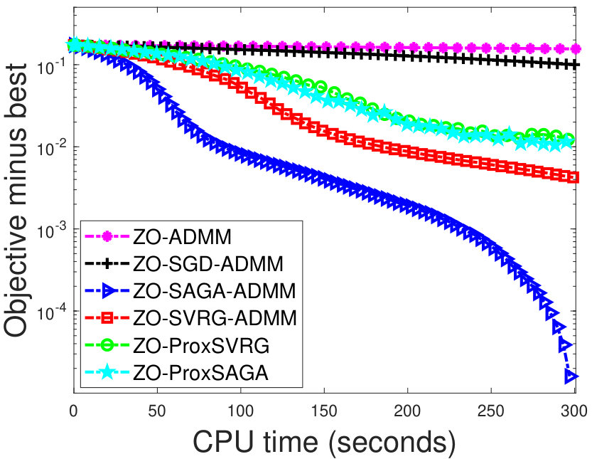 Figure 1
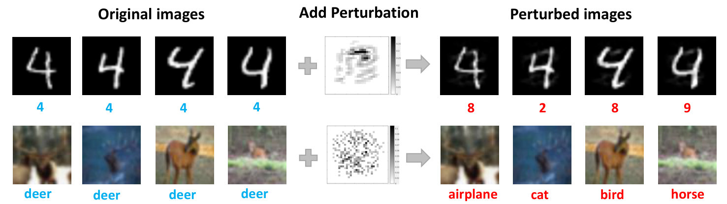 Figure 2
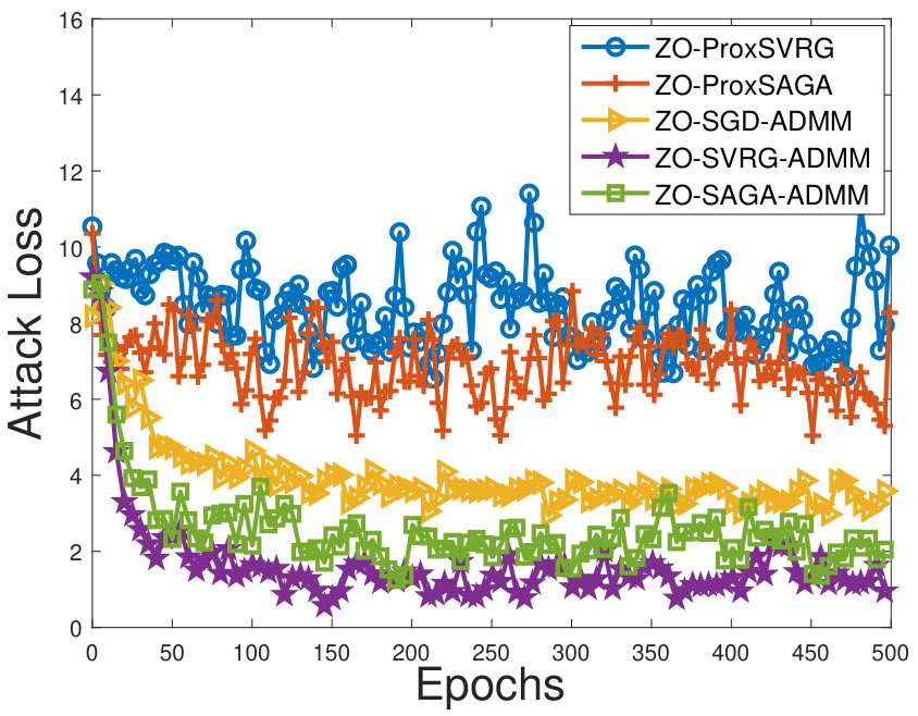 Figure 3
 Figure 4
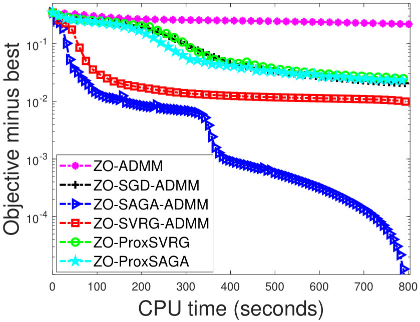 Figure 5
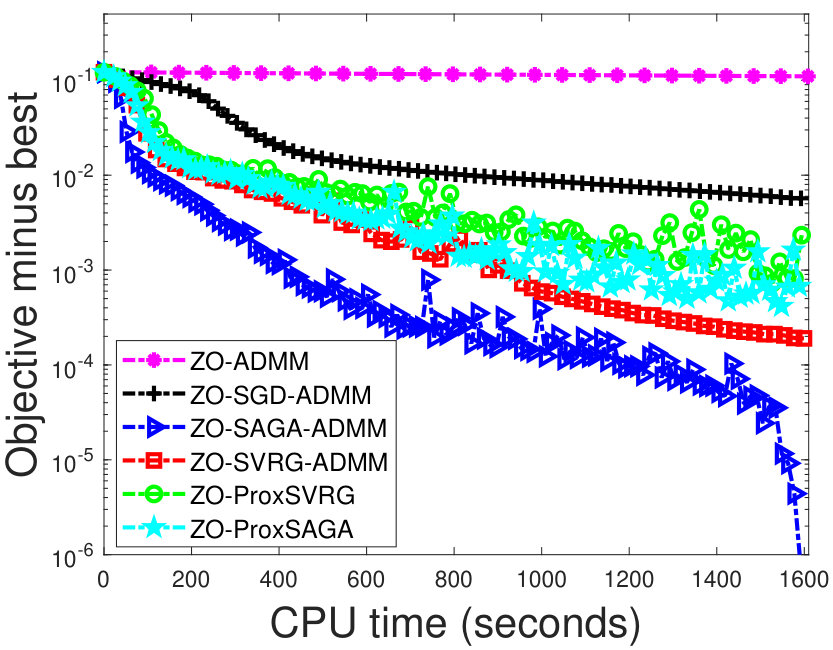 Figure 6
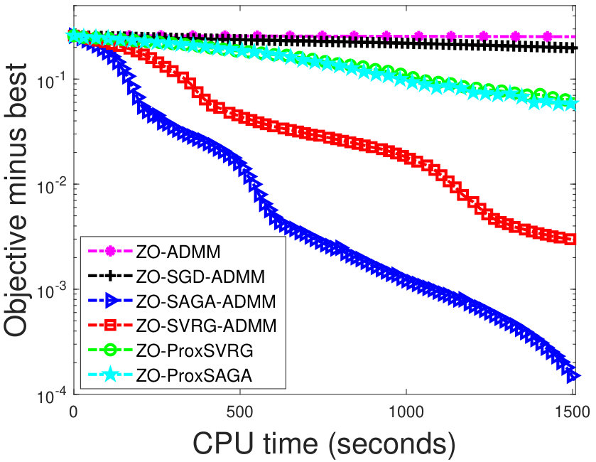 Figure 7
| Algorithm | Reference | Gradient Estimator | Problem | Convergence Rate |
| ZOO-ADMM | Liu et al. (2018a) | GauSGE | C(S) + C(NS) | |
| ZO-GADM | Gao et al. (2018) | UniSGE | C(S) + C(NS) | |
| RSPGF | Ghadimi et al. (2016) | GauSGE | NC(S) + C(NS) | |
| ZO-ProxSVRG | Huang et al. (2019b) | CooSGE | NC(S) + C(NS) | |
| ZO-ProxSAGA | ||||
| ZO-SVRG-ADMM | Ours | CooSGE | NC(S) + C(mNS) | |
| ZO-SAGA-ADMM |
| datasets | #samples | #features | #classes |
|---|---|---|---|
| 20news | 16,242 | 100 | 2 |
| a9a | 32,561 | 123 | 2 |
| w8a | 64,700 | 300 | 2 |
| covtype.binary | 581,012 | 54 | 2 |
Peer Reviews
No public reviews on file for this paper yet. If you reviewed it on a platform where reviews are public (OpenReview, ICLR, NeurIPS, ICML), you can paste yours below so the community can read it here.
Videos
No videos yet. Explain this paper in a talk, walkthrough, or lecture? Add one.
Taxonomy
TopicsStochastic Gradient Optimization Techniques · Sparse and Compressive Sensing Techniques · Machine Learning and ELM
MethodsAlternating Direction Method of Multipliers
Zeroth-Order Stochastic Alternating Direction Method of Multipliers
for Nonconvex Nonsmooth Optimization
Feihu Huang1, Shangqian Gao1, Songcan Chen2,3 and Heng Huang1,4
1 Department of Electrical & Computer Engineering, University of Pittsburgh, USA
2 College of Computer Science & Technology, Nanjing University of Aeronautics and Astronautics
3 MIIT Key Laboratory of Pattern Analysis & Machine Intelligence, China
4 JD Finance America Corporation
[email protected], [email protected], [email protected], [email protected] Corresponding Author.
Abstract
Alternating direction method of multipliers (ADMM) is a popular optimization tool for the composite and constrained problems in machine learning. However, in many machine learning problems such as black-box learning and bandit feedback, ADMM could fail because the explicit gradients of these problems are difficult or even infeasible to obtain. Zeroth-order (gradient-free) methods can effectively solve these problems due to that the objective function values are only required in the optimization. Recently, though there exist a few zeroth-order ADMM methods, they build on the convexity of objective function. Clearly, these existing zeroth-order methods are limited in many applications. In the paper, thus, we propose a class of fast zeroth-order stochastic ADMM methods (i.e., ZO-SVRG-ADMM and ZO-SAGA-ADMM) for solving nonconvex problems with multiple nonsmooth penalties, based on the coordinate smoothing gradient estimator. Moreover, we prove that both the ZO-SVRG-ADMM and ZO-SAGA-ADMM have convergence rate of , where denotes the number of iterations. In particular, our methods not only reach the best convergence rate of for the nonconvex optimization, but also are able to effectively solve many complex machine learning problems with multiple regularized penalties and constraints. Finally, we conduct the experiments of black-box binary classification and structured adversarial attack on black-box deep neural network to validate the efficiency of our algorithms.
1 Introduction
Alternating direction method of multipliers (ADMM Gabay and Mercier (1976); Boyd et al. (2011)) is a popular optimization tool for solving the composite and constrained problems in machine learning. In particular, ADMM can efficiently optimize some problems with complicated structure regularization such as the graph-guided fused lasso Kim et al. (2009), which is too complicated for the other popular optimization methods such as proximal gradient methods Beck and Teboulle (2009). For the large-scale optimization, the stochastic ADMM method Ouyang et al. (2013) has been proposed. Recently, some faster stochastic ADMM methods Suzuki (2014); Zheng and Kwok (2016) have been proposed by using the variance reduced (VR) techniques such as the SVRG Johnson and Zhang (2013). In fact, ADMM is also highly successful in solving various nonconvex problems such as training deep neural networks Taylor et al. (2016). Thus, some fast nonconvex stochastic ADMM methods have been developed in Huang et al. (2016, 2019a).
Currently, most of the ADMM methods need to compute the gradients of objective functions over each iteration. However, in many machine learning problems, the explicit expression of gradient for objective function is difficult or infeasible to obtain. For example, in black-box situations, only prediction results (i.e., function values) are provided Chen et al. (2017); Liu et al. (2018b). In bandit settings Agarwal et al. (2010), player only receives the partial feedback in terms of loss function values, so it is impossible to obtain expressive gradient of the loss function. Clearly, the classic optimization methods, based on the first-order gradient or second-order information, are not competent to these problems. Recently, the zeroth-order optimization methods Duchi et al. (2015); Nesterov and Spokoiny (2017) are developed by only using the function values in the optimization.
In the paper, we focus on using the zeroth-order methods to solve the following nonconvex nonsmooth problem:
[TABLE]
where , for all , is a nonconvex and black-box function, and each is a convex and nonsmooth function. In machine learning, function can be used for the empirical loss, for multiple structure penalties (e.g., sparse + group sparse), and the constraint for encoding the structure pattern of model parameters such as graph structure. Due to the flexibility in splitting the objective function into loss and each penalty , ADMM is an efficient method to solve the obove problem. However, in the problem (1), we only access the objective values rather than the whole explicit function , thus the classic ADMM methods are unsuitable for the problem (1).
Recently, Gao et al. (2018); Liu et al. (2018a) proposed the zeroth-order stochastic ADMM methods, which only use the objective values to optimize. However, these zeroth-order ADMM-based methods build on the convexity of objective function. Clearly, these methods are limited in many nonconvex problems such as adversarial attack on black-box deep neural network (DNN). At the same time, due to that the problem (1) includes multiple nonsmooth regularization functions and an equality constraint, the existing zeroth-order algorithms Liu et al. (2018b); Huang et al. (2019b) are not suitable for solving this problem.
In the paper, thus, we propose a class of fast zeroth-order stochastic ADMM methods (i.e., ZO-SVRG-ADMM and ZO-SAGA-ADMM) to solve the problem (1) based on the coordinate smoothing gradient estimator Liu et al. (2018b). In particular, the ZO-SVRG-ADMM and ZO-SAGA-ADMM methods build on the SVRG Johnson and Zhang (2013) and SAGA Defazio et al. (2014), respectively. Moreover, we study the convergence properties of the proposed methods. Table 1 shows the convergence properties of the proposed methods and other related ones.
1.1 Challenges and Contributions
Although both SVRG and SAGA show good performances in the first-order and second-order methods, applying these techniques to the nonconvex zeroth-order ADMM method is not trivial. There exists at least two main challenges:
- •
Due to failure of the Fejér monotonicity of iteration, the convergence analysis of the nonconvex ADMM is generally quite difficult Wang et al. (2015). With using the inexact zeroth-order estimated gradient, this difficulty becomes greater in the nonconvex ADMM methods.
- •
To guarantee convergence of our zeroth-order ADMM methods, we need to design a new effective Lyapunov function, which can not follow the existing nonconvex (stochastic) ADMM methods Jiang et al. (2019); Huang et al. (2016).
Thus, we carefully establish the Lyapunov functions in the following theoretical analysis to ensure convergence of the proposed methods. In summary, our major contributions are given below:
We propose a class of fast zeroth-order stochastic ADMM methods (i.e., ZO-SVRG-ADMM and ZO-SAGA-ADMM) to solve the problem (1).
- 2)
We prove that both the ZO-SVRG-ADMM and ZO-SAGA-ADMM have convergence rate of for nonconvex nonsmooth optimization. In particular, our methods not only reach the existing best convergence rate for the nonconvex optimization, but also are able to effectively solve many machine learning problems with multiple complex regularized penalties.
- 3)
Extensive experiments conducted on black-box classification and structured adversarial attack on black-box DNNs validate efficiency of the proposed algorithms.
2 Related Works
Zeroth-order (gradient-free) optimization is a powerful optimization tool for solving many machine learning problems, where the gradient of objective function is not available or computationally prohibitive. Recently, the zeroth-order optimization methods are widely applied and studied. For example, zeroth-order optimization methods have been applied to bandit feedback analysis Agarwal et al. (2010) and black-box attacks on DNNs Chen et al. (2017); Liu et al. (2018b). Nesterov and Spokoiny (2017) have proposed several random zeroth-order methods based on the Gaussian smoothing gradient estimator. To deal with the nonsmooth regularization, Gao et al. (2018); Liu et al. (2018a) have proposed the zeroth-order online/stochastic ADMM-based methods.
So far, the above algorithms mainly build on the convexity of problems. In fact, the zeroth-order methods are also highly successful in solving various nonconvex problems such as adversarial attack to black-box DNNs Liu et al. (2018b). Thus, Ghadimi and Lan (2013); Liu et al. (2018b); Gu et al. (2018) have begun to study the zeroth-order stochastic methods for the nonconvex optimization. To deal with the nonsmooth regularization, Ghadimi et al. (2016); Huang et al. (2019b) have proposed some non-convex zeroth-order proximal stochastic gradient methods. However, these methods still are not well competent to some complex machine learning problems such as a task of structured adversarial attack to the black-box DNNs, which is described in the following experiment.
2.1 Notations
Let and for . Given a positive definite matrix , ; and denote the largest and smallest eigenvalues of , respectively, and . and denote the largest and smallest eigenvalues of matrix .
3 Preliminaries
In the section, we begin with restating a standard -approximate stationary point of the problem (1), as in Jiang et al. (2019); Huang et al. (2019a).
Definition 1**.**
Given , the point is said to be an -approximate stationary point of the problems (1), if it holds that
[TABLE]
where ,
[TABLE]
**
Next, we make some mild assumptions regarding problem (1) as follows:
Assumption 1**.**
Each function is -smooth for such that
[TABLE]
which is equivalent to
[TABLE]
Assumption 2**.**
Full gradient of loss function is bounded, i.e., there exists a constant such that for all , it follows that .
Assumption 3**.**
* and for all are all lower bounded, and denote and for .*
Assumption 4**.**
* is a full row or column rank matrix.*
Assumption 1 has been commonly used in the convergence analysis of nonconvex algorithms Ghadimi et al. (2016). Assumption 2 is widely used for stochastic gradient-based and ADMM-type methods Boyd et al. (2011). Assumptions 3 and 4 are usually used in the convergence analysis of ADMM methods Jiang et al. (2019); Huang et al. (2016, 2019a). Without loss of generality, we will use the full column rank of matrix in the rest of this paper.
4 Fast Zeroth-Order Stochastic ADMMs
In this section, we propose a class of zeroth-order stochastic ADMM methods to solve the problem (1). First, we define an augmented Lagrangian function of the problem (1):
[TABLE]
where and denotes the dual variable and penalty parameter, respectively.
In the problem (1), the explicit expression of objective function is not available, and only the function value of is available. To avoid computing explicit gradient, thus, we use the coordinate smoothing gradient estimator Liu et al. (2018b) to estimate gradients: for ,
[TABLE]
where is a coordinate-wise smoothing parameter, and is a standard basis vector with 1 at its -th coordinate, and 0 otherwise.
Based on the above estimated gradients, we propose a zeroth-order ADMM (ZO-ADMM) method to solve the problem (1) by executing the following iterations, for
[TABLE]
where the term with to linearize the term . Here, due to using the inexact zeroth-order gradient to update , we define an approximate function over as follows:
[TABLE]
where , is the zeroth-order gradient and is a step size. Considering the matrix is large, set with to linearize the term . In the problem (1), not only the noisy gradient of is not available, but also the sample size is very large. Thus, we propose fast ZO-SVRG-ADMM and ZO-SAGA-ADMM to solve the problem (1), based on the SVRG and SAGA, respectively.
Algorithm 1 shows the algorithmic framework of ZO-SVRG-ADMM. In Algorithm 1, we use the estimated stochastic gradient with . We have , i.e., this stochastic gradient is a biased estimate of the true full gradient. Although the SVRG has shown a great promise, it relies upon the assumption that the stochastic gradient is an **unbiased **estimate of true full gradient. Thus, adapting the similar ideas of SVRG to zeroth-order ADMM optimization is not a trivial task. To handle this challenge, we choose the appropriate step size , penalty parameter and smoothing parameter to guarantee the convergence of our algorithms, which will be discussed in the following convergence analysis.
Algorithm 2 shows the algorithmic framework of ZO-SAGA-ADMM. In Algorithm 2, we use the estimated stochastic gradient \hat{g}_{t}=\frac{1}{b}\sum_{i_{t}\in\mathcal{I}_{t}}\big{(}\hat{\nabla}f_{i_{t}}(x_{t})-\hat{\nabla}f_{i_{t}}(z^{t}_{i_{t}})\big{)}+\hat{\phi}_{t} with . Similarly, we have .
5 Convergence Analysis
In this section, we will study the convergence properties of the proposed algorithms (ZO-SVRG-ADMM and ZO-SAGA-ADMM).
5.1 Convergence Analysis of ZO-SVRG-ADMM
In this subsection, we analyze convergence properties of the ZO-SVRG-ADMM.
Given the sequence generated from Algorithm 1, we define a Lyapunov function:
[TABLE]
where the positive sequence satisfies
[TABLE]
Next, we definite a useful variable \theta^{s}_{t}\!=\!\mathbb{E}\big{[}\|x^{s}_{t+1}-x^{s}_{t}\|^{2}+\|x^{s}_{t}-x^{s}_{t-1}\|^{2}+\frac{d}{b}(\|x^{s}_{t}-\tilde{x}^{s}\|^{2}+\|x^{s}_{t-1}-\tilde{x}^{s}\|^{2})+\sum_{j=1}^{k}\|y_{j}^{s,t}-y_{j}^{s,t+1}\|^{2}\big{]}.
Theorem 1**.**
Suppose the sequence is generated from Algorithm 1. Let , , and , then we have
[TABLE]
where , and is a lower bound of function . It follows that suppose the smoothing parameter and the whole iteration number satisfy
[TABLE]
then is an -approximate stationary point of the problems (1), where .
Remark 1**.**
Theorem 1 shows that given , , , and , the ZO-SVRG-ADMM has convergence rate of . Specifically, when , given , the ZO-SVRG-ADMM has convergence rate of ; when , given , it has convergence rate of ; when , given , it has convergence rate of .
5.2 Convergence Analysis of ZO-SAGA-ADMM
In this subsection, we provide the convergence analysis of the ZO-SAGA-ADMM.
Given the sequence generated from Algorithm 2, we define a Lyapunov function
[TABLE]
Here the positive sequence satisfies
[TABLE]
where denotes probability of an index in . Next, we definite a useful variable \theta_{t}\!=\!\mathbb{E}\big{[}\|x_{t+1}\!-\!x_{t}\|^{2}\!+\!\|x_{t}\!-\!x_{t-1}\|^{2}\!+\!\frac{d}{bn}\sum^{n}_{i=1}(\|x_{t}\!-\!z^{t}_{i}\|^{2}\!+\!\|x_{t-1}\!-\!z^{t-1}_{i}\|^{2})\!+\!\sum_{j=1}^{k}\|y_{j}^{t}\!-\!y_{j}^{t+1}\|^{2}\big{]}.
Theorem 2**.**
Suppose the sequence is generated from Algorithm 2. Let , and then we have
[TABLE]
where , and is a lower bound of function . It follows that suppose the parameters and satisfy
[TABLE]
then is an -approximate stationary point of the problems (1), where .
Remark 2**.**
Theorem 2 shows that , , and , the ZO-SAGA-ADMM has the of convergence rate. Specifically, when , given , the ZO-SAGA-ADMM has convergence rate of ; when , given , it has convergence rate of ; when , given , it has convergence rate of .
6 Experiments
In this section, we compare our algorithms (ZO-SVRG-ADMM, ZO-SAGA-ADMM) with the ZO-ProxSVRG, ZO-ProxSAGA Huang et al. (2019b), the deterministic zeroth-order ADMM (ZO-ADMM), and zeroth-order stochastic ADMM (ZO-SGD-ADMM) without variance reduction on two applications: 1) robust black-box binary classification, and 2) structured adversarial attacks on black-box DNNs.
6.1 Robust Black-Box Binary Classification
In this subsection, we focus on a robust black-box binary classification task with graph-guided fused lasso. Given a set of training samples , where and , we find the optimal parameter by solving the problem:
[TABLE]
where is the black-box loss function, that only returns the function value given an input. Here, we specify the loss function f_{i}(x)=\frac{\sigma^{2}}{2}\big{(}1-\exp(-\frac{(l_{i}-a_{i}^{T}x)^{2}}{\sigma^{2}})\big{)}, which is the nonconvex robust correntropy induced loss He et al. (2011). Matrix decodes the sparsity pattern of graph obtained by learning sparse Gaussian graphical model Huang and Chen (2015). In the experiment, we give mini-batch size , smoothing parameter and penalty parameters .
In the experiment, we use some public real datasets11120news is from https://cs.nyu.edu/~roweis/data.html; others are from www.csie.ntu.edu.tw/~cjlin/libsvmtools/datasets/., which are summarized in Table 2. For each dataset, we use half of the samples as training data and the rest as testing data. Figure 1 shows that the objective values of our algorithms faster decrease than the other algorithms, as the CPU time increases. In particular, our algorithms show better performances than the zeroth-order proximal algorithms. It is relatively difficult that these zeroth-order proximal methods deal with the nonsmooth penalties in the problem (6). Thus, we have to use some iterative methods to solve the proximal operator in these proximal methods.
6.2 Structured Attacks on Black-Box DNNs
In this subsection, we use our algorithms to generate adversarial examples to attack the pre-trained DNN models, whose parameters are hidden from us and only its outputs are accessible. Moreover, we consider an interesting problem: “What possible structures could adversarial perturbations have to fool black-box DNNs ?” Thus, we use the zeroth-order algorithms to find an universal structured adversarial perturbation that could fool the samples , which can be regarded as the following problem:
[TABLE]
where represents the final layer output before softmax of neural network, and ensures the validness of created adversarial examples. Specifically, if for all and , otherwise . Following Xu et al. (2018), we use the overlapping lasso to obtain structured perturbations. Here, the overlapping groups generate from dividing an image into sub-groups of pixels.
In the experiment, we use the pre-trained DNN models on MNIST and CIFAR-10 as the target black-box models, which can attain and test accuracy, respectively. For MNIST, we select 20 samples from a target class and set batch size ; For CIFAR-10, we select 30 samples and set . In the experiment, we set , where and for MNIST and CIFAR-10, respectively. At the same time, we set the parameters , , and . For both datasets, the kernel size for overlapping group lasso is set to and the stride is one.
Figure 3 shows that attack losses (i.e. the first term of the problem (6.2)) of our methods faster decrease than the other methods, as the number of iteration increases. Figure 2 shows that our algorithms can learn some structure perturbations, and can successfully attack the corresponding DNNs.
7 Conclusions
In the paper, we proposed fast ZO-SVRG-ADMM and ZO-SAGA-ADMM methods based on the coordinate smoothing gradient estimator, which only uses the objective function values to optimize. Moreover, we prove that the proposed methods have a convergence rate of . In particular, our methods not only reach the existing best convergence rate for the nonconvex optimization, but also are able to effectively solve many machine learning problems with the complex nonsmooth regularizations.
Acknowledgments
F.H., S.G., H.H. were partially supported by U.S. NSF IIS 1836945, IIS 1836938, DBI 1836866, IIS 1845666, IIS 1852606, IIS 1838627, IIS 1837956. S.C. was partially supported by the NSFC under Grant No. 61806093 and No. 61682281, and the Key Program of NSFC under Grant No. 61732006.
Appendix A Supplementary Materials
In this section, we study at detail the convergence properties of both the ZO-SVRG-ADMM and ZO-SAGA-ADMM algorithms.
Notations: To make the paper easier to follow, we give the following notations:
- •
and for all .
- •
denotes the vector norm and the matrix spectral norm, respectively.
- •
, where is a positive definite matrix.
- •
and denote the minimum and maximum eigenvalues of , respectively.
- •
denotes the maximum eigenvalues of for all , and .
- •
and denote the minimum and maximum eigenvalues of matrix , respectively; the conditional number .
- •
and denote the minimum and maximum eigenvalues of matrix for all , respectively; and .
- •
denotes the smoothing parameter of the gradient estimator.
- •
denotes the step size of updating variable .
- •
denotes the Lipschitz constant of .
- •
denotes the mini-batch size of stochastic gradient.
- •
, and are the total number of iterations, the number of iterations in the inner loop, and the number of iterations in the outer loop, respectively.
A.1 Theoretical Analysis of the ZO-SVRG-ADMM
In this subsection, we in detail give the convergence analysis of the ZO-SVRG-ADMM algorithm. First, we give some useful lemmas as follows:
Lemma 1**.**
Suppose the sequence \big{\{}(x^{s}_{t},y_{[k]}^{s,t},\lambda^{s}_{t})_{t=1}^{m}\big{\}}_{s=1}^{S} is generated by Algorithm 1, the following inequality holds
[TABLE]
Proof.
Using the optimal condition for the step 9 of Algorithm 1, we have
[TABLE]
By the step 11 of Algorithm 1, we have
[TABLE]
It follows that
[TABLE]
where is the pseudoinverse of . By Assumption 4, i.e., is a full column matrix, we have . Then we have
[TABLE]
where denotes the minimum eigenvalues of .
Next, considering the upper bound of , we have
[TABLE]
where the second inequality holds by Lemma 1 of Huang et al. [2019b] and the third inequality holds by Assumption 1. Finally, combining (A.1) and (A.1), we obtain the above result. ∎
Lemma 2**.**
Suppose the sequence is generated from Algorithm 1, and define a Lyapunov function:
[TABLE]
where the positive sequence satisfies, for
[TABLE]
It follows that
[TABLE]
where , , and denotes a lower bound of .
Proof.
By the optimal condition of step 8 in Algorithm 1, we have, for
[TABLE]
where the first inequality holds by the convexity of function , and the second equality follows by applying the equality on the term . Thus, we have, for all
[TABLE]
Telescoping inequality (17) over from to , we obtain
[TABLE]
where .
By Assumption 1, we have
[TABLE]
Using the optimal condition of the step 9 in Algorithm 1, we have
[TABLE]
Combining (19) and (20), we have
[TABLE]
where the equality holds by applying the equality on the term , the inequality holds by the inequality , and the inequality holds by Lemma 1 of Huang et al. [2019b]. Thus, we obtain
[TABLE]
Using the step 10 in Algorithm 1, we have
[TABLE]
Combining (18), (22) and (A.1), we have
[TABLE]
Next, we define a Lyapunov function as follows:
[TABLE]
Considering the upper bound of , we have
[TABLE]
where the above inequality holds by the Cauchy-Schwarz inequality with . Combining (25) with (A.1), then we obtain
[TABLE]
where and .
Next, we will prove the relationship between and . Due to , we have
[TABLE]
It follows that
[TABLE]
where the first inequality holds by the inequality ; the third inequality holds by the definition of zeroth-order gradient (4).
By Lemma 1, we have
[TABLE]
Since , for all and , by (18), we have
[TABLE]
By (22), we have
[TABLE]
By (A.1), we have
[TABLE]
where the second inequality holds by (A.1).
Combining (A.1), (32) with (A.1), we have
[TABLE]
Therefore, we have
[TABLE]
where , and .
Let and , recursing on , we have
[TABLE]
where the above inequality holds by is an increasing function and . It follows that, for
[TABLE]
When , let , (i.e., ) and , we have . Further, let and , we have
[TABLE]
where the second inequality follows . Thus, we have for all .
When , let , (i.e., ) and , we have . Further, let and , we have
[TABLE]
where the second equality follows by . Thus, we have .
When , let , (i.e., ) and , we have . Further, let and , we have
[TABLE]
where the second equality follows by . Thus, we have .
By Assumption 4. i.e., is a full column rank matrix, we have . It follows that . Since , we have
[TABLE]
where the first inequality is obtained by applying to the terms , and with , respectively; the second inequality follows by Lemma 1 of Huang et al. [2019b] and Assumption 2. Using the definition of function and Assumption 3, we have
[TABLE]
Thus the function is bounded from below. Let denotes a lower bound of .
Finally, telescoping (A.2) and (A.1) over from [math] to and over from to , we have
[TABLE]
where and .
∎
Next, based on the above lemmas, we give the convergence analysis of ZO-SVRG-ADMM algorithm. For notational simplicity, let
[TABLE]
Theorem 3**.**
Suppose the sequence is generated from Algorithm 1. Let , , and , then we have
[TABLE]
where with , and is a lower bound of function . It follows that suppose the smoothing parameter and the whole iteration number satisfy
[TABLE]
then is an -approximate solution of (1), where .
Proof.
First, we define a useful variable \theta^{s}_{t}=\mathbb{E}\big{[}\|x^{s}_{t+1}-x^{s}_{t}\|^{2}+\|x^{s}_{t}-x^{s}_{t-1}\|^{2}+\frac{d}{b}(\|x^{s}_{t}-\tilde{x}^{s}\|^{2}+\|x^{s}_{t-1}-\tilde{x}^{s}\|^{2})+\sum_{j=1}^{k}\|y_{j}^{s,t}-y_{j}^{s,t+1}\|^{2}\big{]}. By the step 8 of Algorithm 1, we have, for all
[TABLE]
where the first inequality follows by the inequality .
By the step 9 of Algorithm 1, we have
[TABLE]
By the step 10 of Algorithm 1, we have
[TABLE]
Next, combining the above inequalities (A.1), (A.1) and (A.1), we have
[TABLE]
where the third inequality holds by Lemma 2, , , and .
Given and , it is easy verifies that and , which are independent on and . Thus, we obtain
[TABLE]
∎
A.2 Theoretical Analysis of the ZO-SAGA-ADMM
In this subsection, we in detail give the convergence analysis of the ZO-SAGA-ADMM algorithm. We begin with giving some useful lemmas as follows:
Lemma 3**.**
Suppose the sequence is generated by Algorithm 2. The following inequality holds
[TABLE]
Proof.
By the optimize condition of the the step 7 in Algorithm 2, we have
[TABLE]
Using the step 8 of Algorithm 2, then we have
[TABLE]
It follows that
[TABLE]
where is the pseudoinverse of . By Assumption 4, i.e., is a full column matrix, we have . Then we have
[TABLE]
Next, considering the upper bound of , we have
[TABLE]
where the second inequality holds by lemma 3 of Huang et al. [2019b], and the third inequality holds by Assumption 1.
Finally, combining the inequalities (A.2) and (A.2), we can obtain the above result. ∎
Lemma 4**.**
Suppose the sequence is generated from Algorithm 2, and define a Lyapunov function
[TABLE]
where the positive sequence satisfies
[TABLE]
It follows that
[TABLE]
where and , and denotes a lower bound of .
Proof.
By the optimal condition of step 6 in Algorithm 2, we have, for
[TABLE]
where the first inequality holds by the convexity of function , and the second equality follows by applying the equality on the term . Thus, we have, for all
[TABLE]
Telescoping inequality (57) over from to , we obtain
[TABLE]
where .
By Assumption 1, we have
[TABLE]
Using the step 7 of Algorithm 2, we have
[TABLE]
Combining (59) and (60), we have
[TABLE]
where the equality holds by applying the equality on the term ; the inequality follows by the inequality , and the inequality holds by lemma 3 of Huang et al. [2019b]. Thus, we obtain
[TABLE]
By the step 8 in Algorithm 2, we have
[TABLE]
Combining (58), (A.2) and (A.2), we have
[TABLE]
Next, we define a Lyapunov function as follows:
[TABLE]
By the step 9 of Algorithm 2, we have
[TABLE]
where denotes probability of an index being in . Here, we have
[TABLE]
where the first inequality follows from , and the second inequality holds by . Considering the upper bound of , we have
[TABLE]
where . Combining (A.2) with (A.2), we have
[TABLE]
It follows that
[TABLE]
where .
Let and . Since and , it follows that
[TABLE]
where . Then recursing on , for , we have
[TABLE]
It follows that
[TABLE]
When , let (i.e., ) and , we have . Further, let and , we have
[TABLE]
Thus, we have .
When , let (i.e., ) and , we have . Further, let and , we have
[TABLE]
Thus, we have .
When , let (i.e.,) and , we have . Further, let and , we have
[TABLE]
Thus, we have .
By Assumption 4, i.e., is a full column rank matrix, we have . It follows that . Since \lambda_{t+1}=(A^{T})^{+}\big{(}\hat{g}_{t}+\frac{G}{\eta}(x_{t+1}-x_{t})\big{)}, we have
[TABLE]
where the first inequality is obtained by applying to the terms , and with , respectively; the second inequality follows by Lemma 3 of Huang et al. [2019b] and Assumption 2. By definition of the function and Assumption 3, we have
[TABLE]
Thus, the function is bounded from below. Let denotes a lower bound of .
Finally, telescoping inequality (A.2) over from [math] to , we have
[TABLE]
where and .
∎
Next, based on the above lemmas, we give the convergence properties of the ZO-SAGA-ADMM algorithm. For notational simplicity, let
[TABLE]
Theorem 4**.**
Suppose the sequence is generated from Algorithm 2. Let , and then we have
[TABLE]
where with , and is a lower bound of function . It follows that suppose the parameters and satisfy
[TABLE]
then is an -approximate solution of (1), where .
Proof.
We begin with defining an useful variable \theta_{t}=\mathbb{E}\big{[}\|x_{t+1}-x_{t}\|^{2}+\|x_{t}-x_{t-1}\|^{2}+\frac{d}{bn}\sum^{n}_{i=1}(\|x_{t}-z^{t}_{i}\|^{2}+\|x_{t-1}-z^{t-1}_{i}\|^{2})+\sum_{j=1}^{k}\|y_{j}^{t}-y_{j}^{t+1}\|^{2}\big{]}. By the optimal condition of the step 6 in Algorithm 2, we have, for all
[TABLE]
where the first inequality follows by the inequality .
By the step 7 in Algorithm 2, we have
[TABLE]
By the step 8 of Algorithm 2, we have
[TABLE]
where the first inequality holds by Lemma 3.
Next, combining the above inequalities (A.2), (A.2) and (A.2), we have
[TABLE]
where the third inequality holds by Lemma 4, and , , and .
Given and , since is relatively small, it is easy verifies that and , which are independent on and . Thus, we obtain
[TABLE]
∎
The reference list from the paper itself. Each links out to its DOI / PubMed record.
- 1Agarwal et al. [2010] Alekh Agarwal, Ofer Dekel, and Lin Xiao. Optimal algorithms for online convex optimization with multi-point bandit feedback. In COLT , pages 28–40. Citeseer, 2010.
- 2Beck and Teboulle [2009] Amir Beck and Marc Teboulle. A fast iterative shrinkage-thresholding algorithm for linear inverse problems. SIAM journal on imaging sciences , 2(1):183–202, 2009.
- 3Boyd et al. [2011] Stephen Boyd, Neal Parikh, Eric Chu, Borja Peleato, and Jonathan Eckstein. Distributed optimization and statistical learning via the alternating direction method of multipliers. Foundations and Trends® in Machine Learning , 3(1):1–122, 2011.
- 4Chen et al. [2017] Pin-Yu Chen, Huan Zhang, Yash Sharma, Jinfeng Yi, and Cho-Jui Hsieh. Zoo: Zeroth order optimization based black-box attacks to deep neural networks without training substitute models. In Workshop on Artificial Intelligence and Security , pages 15–26. ACM, 2017.
- 5Defazio et al. [2014] Aaron Defazio, Francis Bach, and Simon Lacoste-Julien. Saga: A fast incremental gradient method with support for non-strongly convex composite objectives. In NIPS , pages 1646–1654, 2014.
- 6Duchi et al. [2015] John C Duchi, Michael I Jordan, Martin J Wainwright, and Andre Wibisono. Optimal rates for zero-order convex optimization: The power of two function evaluations. IEEE TIT , 61(5):2788–2806, 2015.
- 7Gabay and Mercier [1976] Daniel Gabay and Bertrand Mercier. A dual algorithm for the solution of nonlinear variational problems via finite element approximation. Computers & Mathematics with Applications , 2(1):17–40, 1976.
- 8Gao et al. [2018] Xiang Gao, Bo Jiang, and Shuzhong Zhang. On the information-adaptive variants of the admm: an iteration complexity perspective. Journal of Scientific Computing , 76(1):327–363, 2018.