TL;DR
This paper identifies an unexpected cooling delay in high-mass white dwarfs, not explained by current models, and suggests $^{22}$Ne settling as a possible cause, challenging existing white dwarf cooling theories.
Contribution
It reveals a significant extra cooling delay in high-mass white dwarfs and proposes $^{22}$Ne settling as a potential explanation, advancing understanding of white dwarf evolution.
Findings
Approximately 6% of high-mass WDs experience an 8 Gyr cooling delay.
The delay cannot be explained by crystallization or mergers alone.
$^{22}$Ne settling may account for the additional cooling delay.
Abstract
Recently, the power of Gaia data has revealed an enhancement of high-mass white dwarfs (WDs) on the Hertzsprung--Russell diagram, called the Q branch. This branch is located at the high-mass end of the recently identified crystallization branch. Investigating its properties, we find that the number density and velocity distribution on the Q branch cannot be explained by the cooling delay of crystallization alone, suggesting the existence of an extra cooling delay. To quantify this delay, we statistically compare two age indicators -- the dynamical age inferred from transverse velocity, and the photometric isochrone age -- for more than one thousand high-mass WDs (1.08--1.23 ) selected from Gaia Data Release 2. We show that about 6 % of the high-mass WDs must experience an 8 Gyr extra cooling delay on the Q branch, in addition to the crystallization and merger delays. This…
Click any figure to enlarge with its caption.
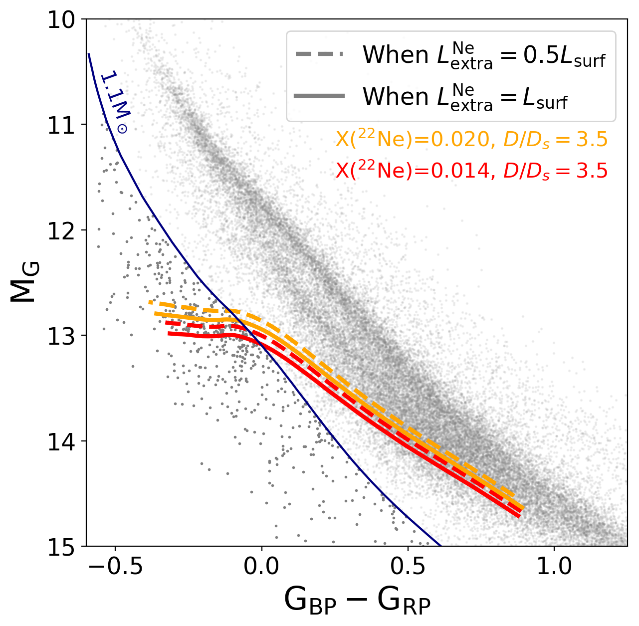 Figure 1
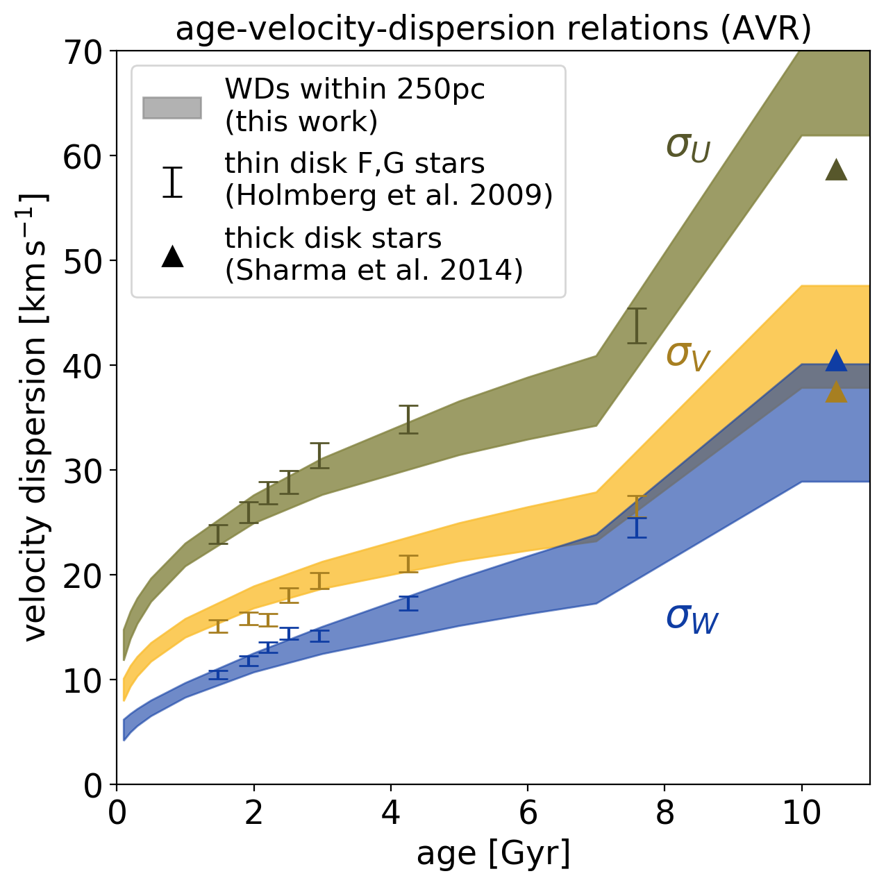 Figure 2
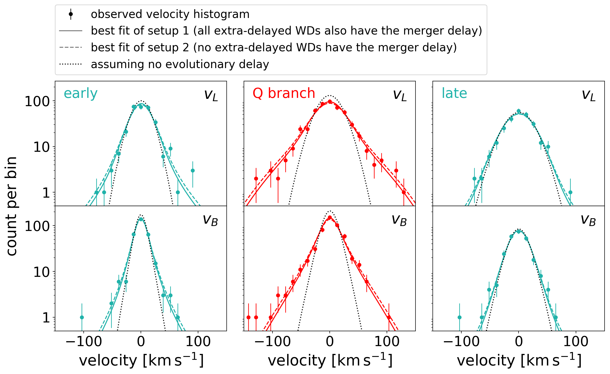 Figure 3
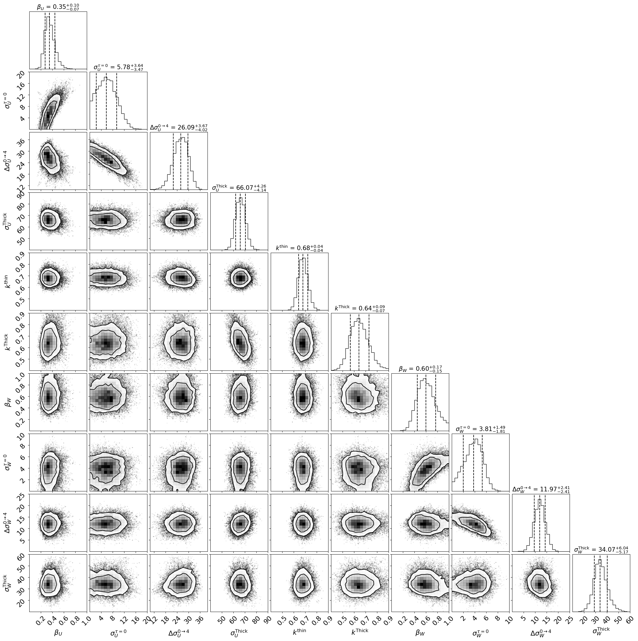 Figure 4
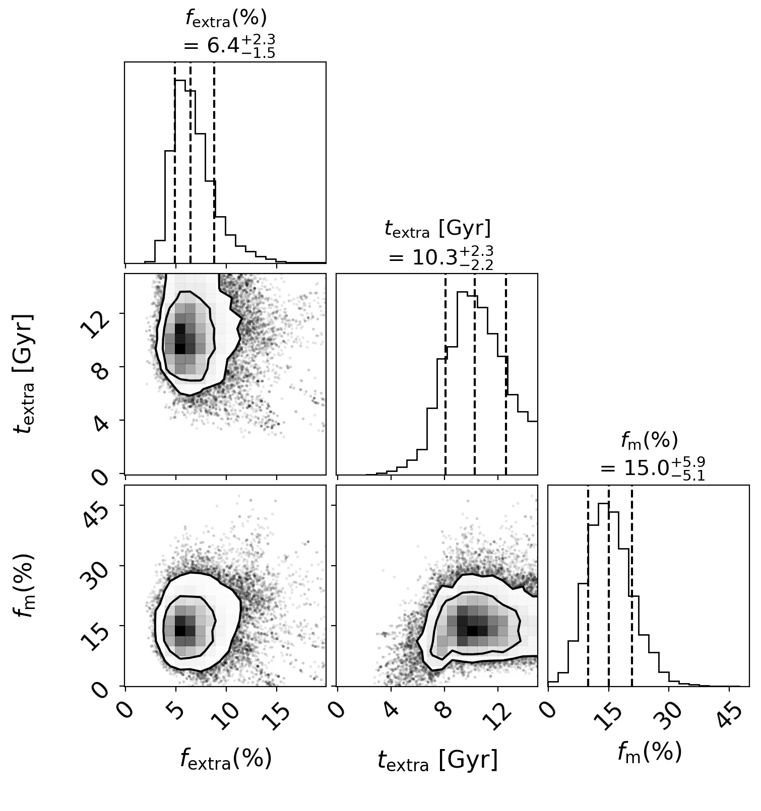 Figure 5
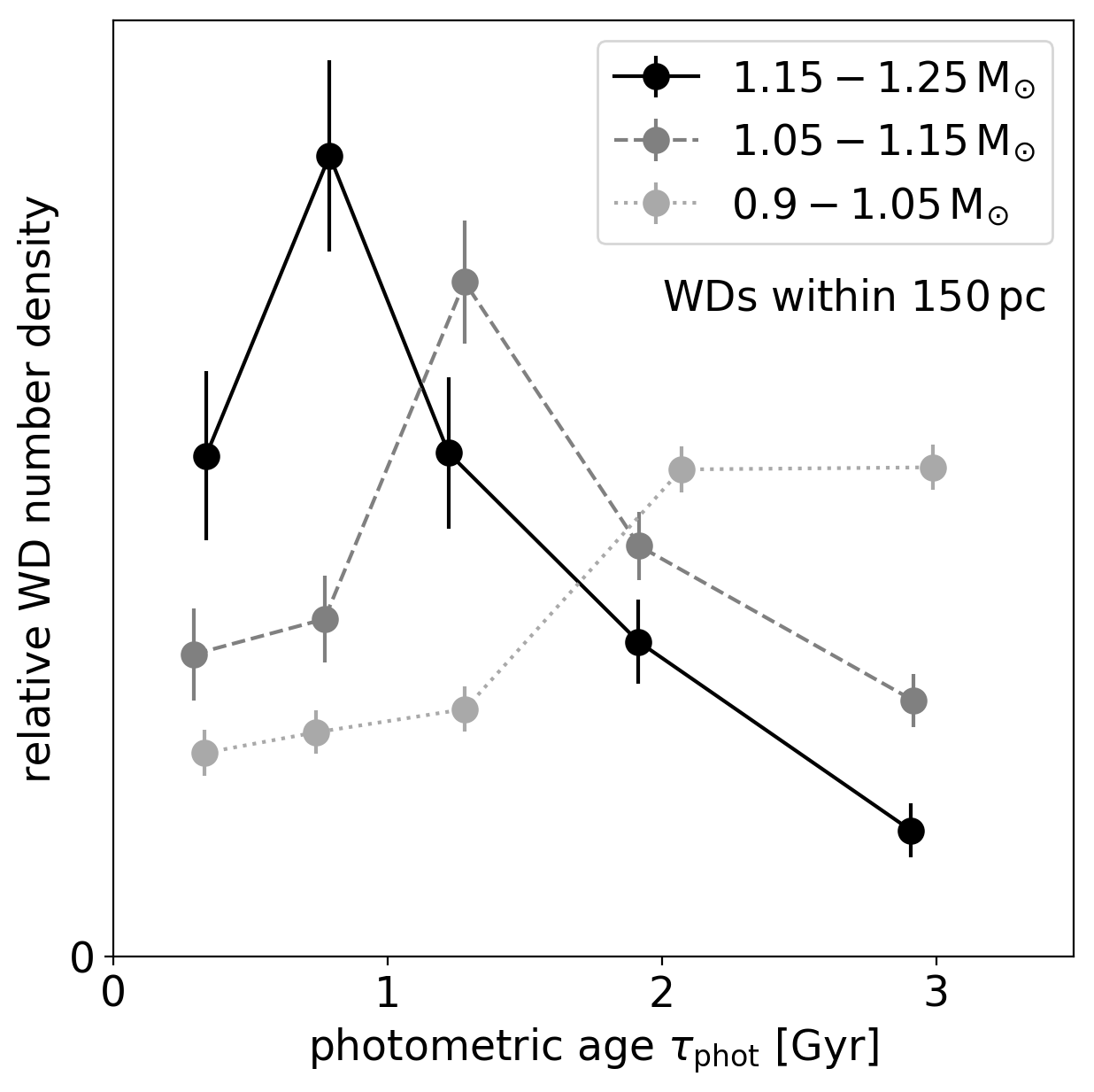 Figure 6
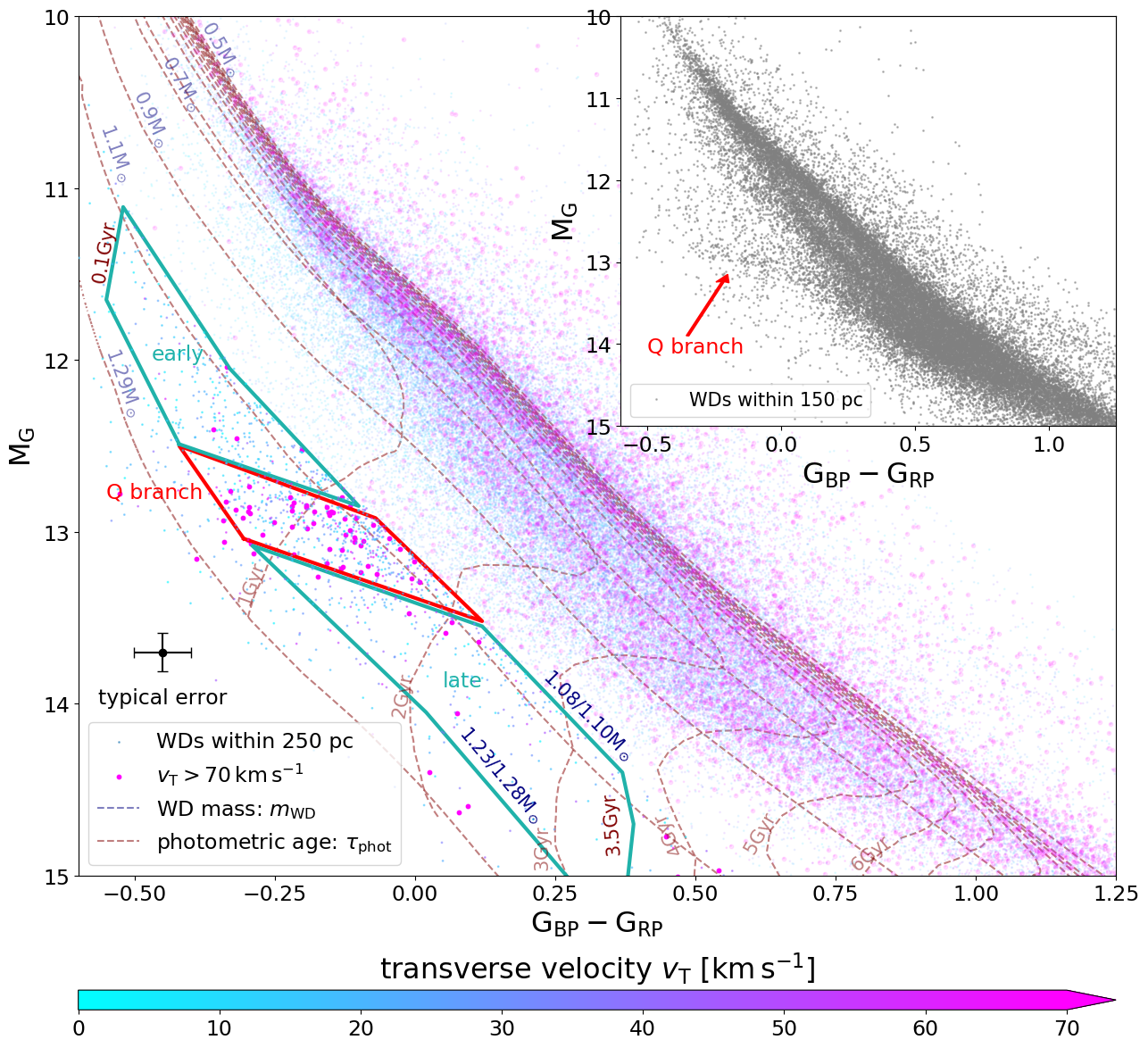 Figure 1
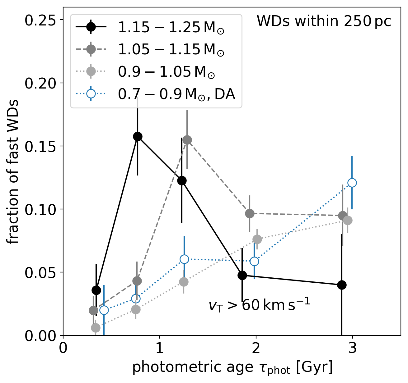 Figure 3
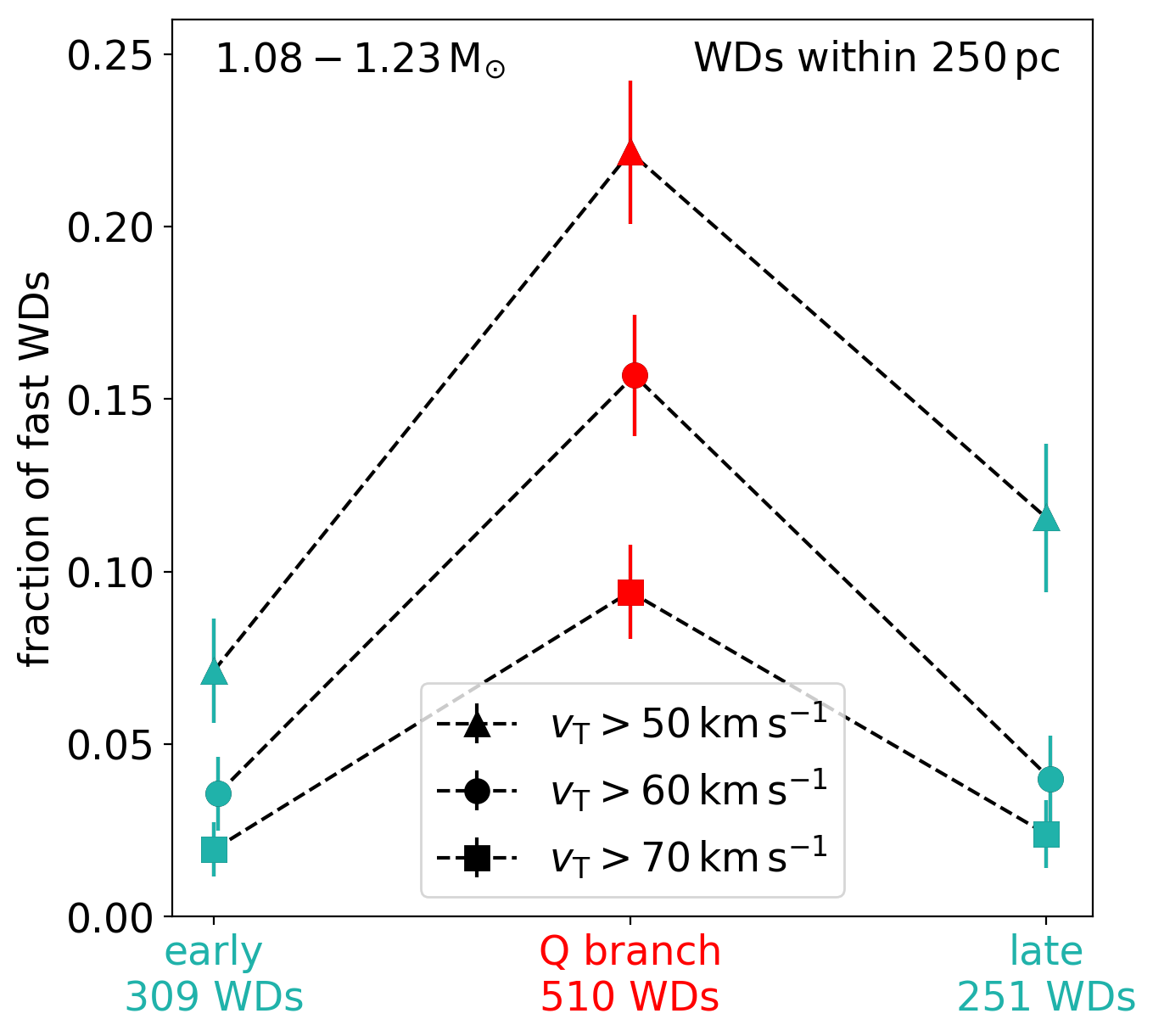 Figure 3
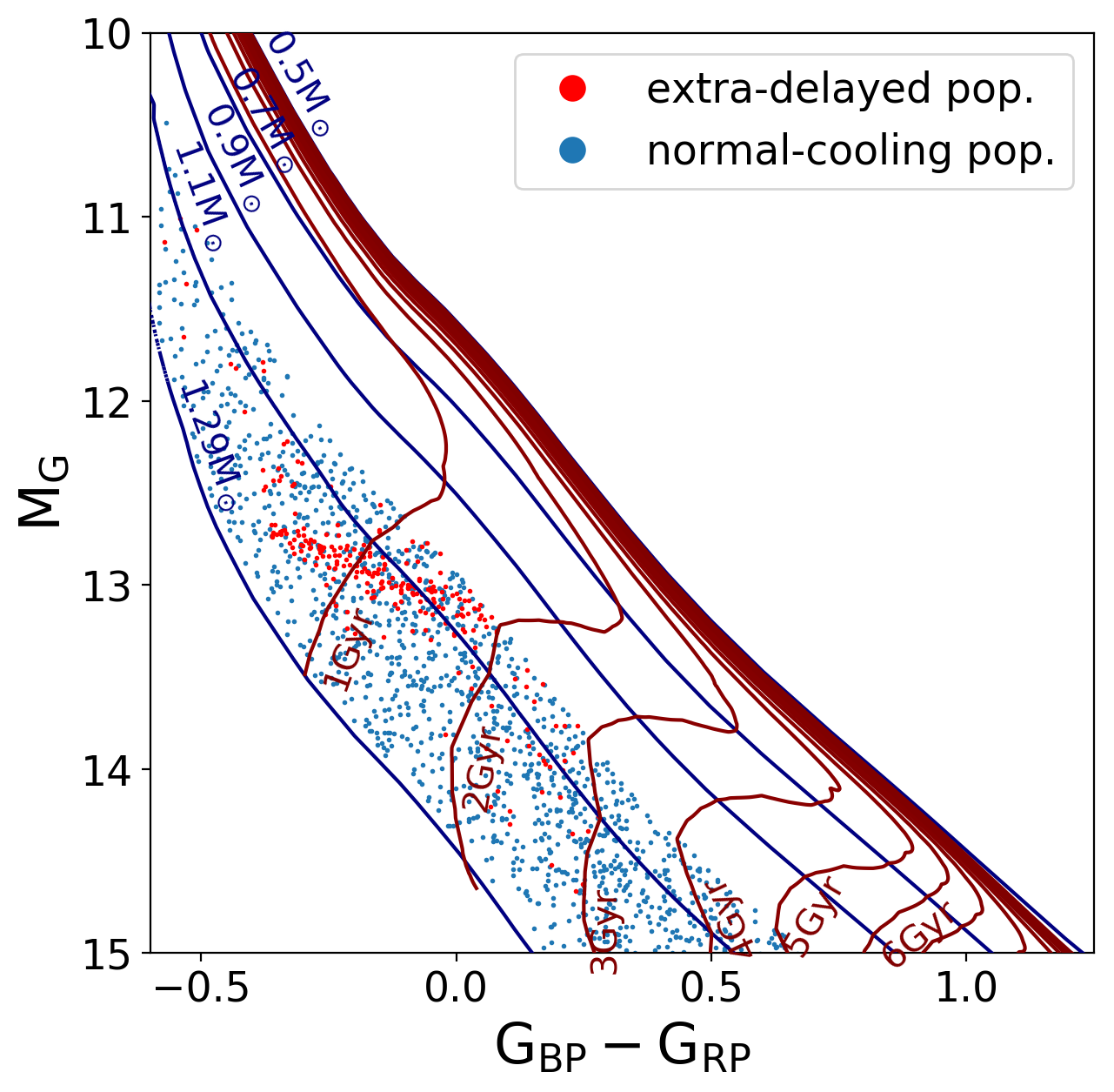 Figure 4
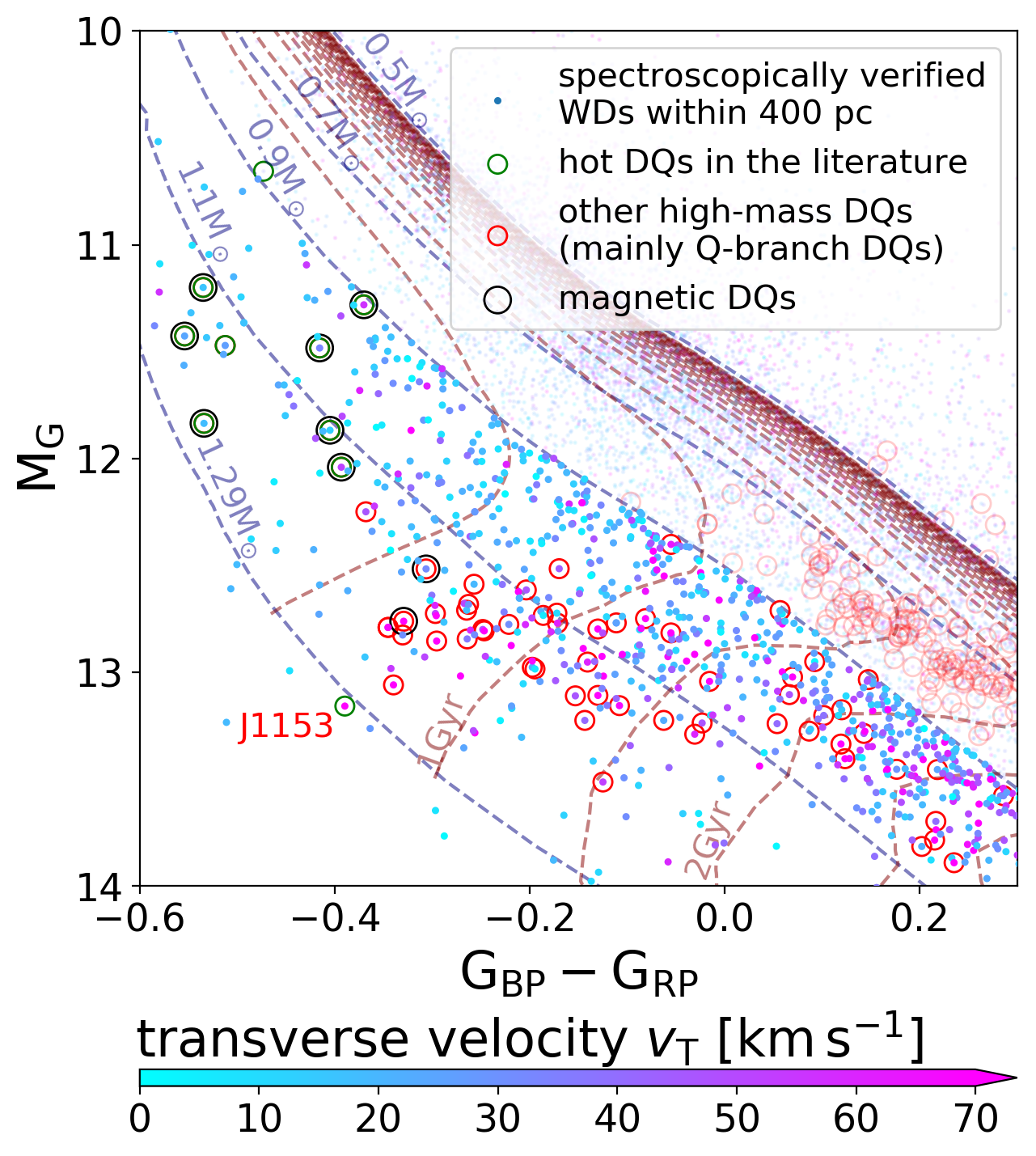 Figure 9
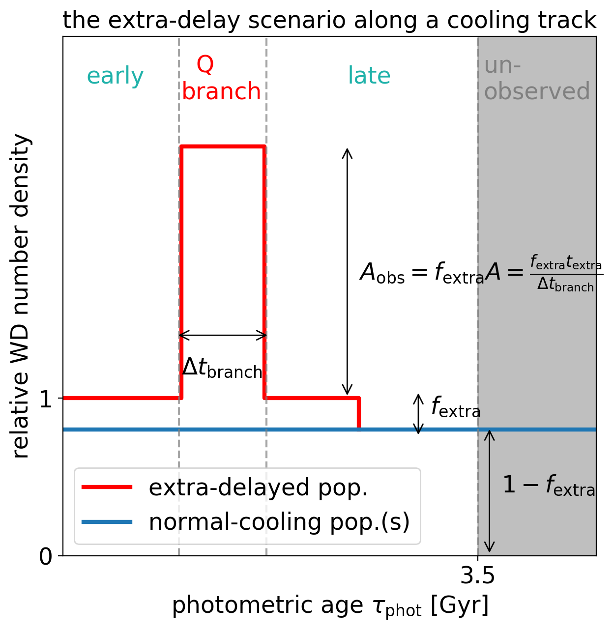 Figure 12
| Population | single-star evolution | extra-delayed | double-WD merger products with normal-cooling |
|---|---|---|---|
| (abbreviation) | (s) | (extra) | (m) |
| merger delay | no | yes or no (setup 1 or 2) | yes |
| extra cooling delay | no | yes | no |
| early | 0 | or 0 | |
| Q branch | 0 | or | |
| late | 0 | or |
| 250 pc spectro- | all | DQ | DA |
|---|---|---|---|
| scopic sample | |||
| all | 76 | 19 | 53 |
| 23 | 8 | 14 | |
| 16 | 7 | 8 | |
| 9 | 2 | 6 | |
Peer Reviews
No public reviews on file for this paper yet. If you reviewed it on a platform where reviews are public (OpenReview, ICLR, NeurIPS, ICML), you can paste yours below so the community can read it here.
Code & Models
Videos
No videos yet. Explain this paper in a talk, walkthrough, or lecture? Add one.
A Cooling Anomaly of High-Mass White Dwarfs
Department of Physics and Astronomy, The Johns Hopkins University, 3400 N Charles Street, Baltimore, MD 21218, USA
Department of Physics and Astronomy, The Johns Hopkins University, 3400 N Charles Street, Baltimore, MD 21218, USA
Brice Ménard
Department of Physics and Astronomy, The Johns Hopkins University, 3400 N Charles Street, Baltimore, MD 21218, USA
Kavli Institute for the Physics and Mathematics of the Universe, University of Tokyo, Kashiwa 277-8583, Japan
(Received 2019 June 6; Revised 2019 September 1; Accepted 2019 September 4)
Abstract
Recently, the power of Gaia data has revealed an enhancement of high-mass white dwarfs (WDs) on the Hertzsprung–Russell diagram, called the Q branch. This branch is located at the high-mass end of the recently identified crystallization branch. Investigating its properties, we find that the number density and velocity distribution on the Q branch cannot be explained by the cooling delay of crystallization alone, suggesting the existence of an extra cooling delay. To quantify this delay, we statistically compare two age indicators – the dynamical age inferred from transverse velocity, and the photometric isochrone age – for more than one thousand high-mass WDs (1.08–1.23 ) selected from Gaia Data Release 2. We show that about of the high-mass WDs must experience an 8 Gyr extra cooling delay on the Q branch, in addition to the crystallization and merger delays. This cooling anomaly is a challenge for WD cooling models. We point out that settling in C/O-core WDs could account for this extra cooling delay.
White dwarf stars (1799); Hertzsprung Russell diagram (725); Stellar kinematics (1608); Stellar ages (1581); Milky Way disk (1050); Bayesian statistics (1900)
††journal: ApJ††software: astropy package (Astropy Collaboration et al., 2013, 2018), corner.py (Foreman-Mackey, 2016), emcee (Foreman-Mackey et al., 2013), numpy (Oliphant, 2006), matplotlib (Hunter, 2007), SciPy (Virtanen et al., 2019)
1 Introduction
Until recently, explorations of the white dwarf region in the Hertzsprung–Russell (H–R) diagram were severely limited by the number of objects with available distance estimates. The European Space Agency Gaia mission (Gaia Collaboration et al., 2016) has changed this situation drastically. Gaia is an all-sky survey of astrometry and photometry for stars down to 20.7 magnitude. The H–R diagram of white dwarfs generated by Gaia Data Release 2 (DR2) reveals three branch-like features, called the A, B, and Q branches111Named after the presence of DA, DB, and DQ white dwarfs (Gaia Collaboration et al., 2018a), respectively. DA white dwarfs have hydrogen lines in their spectr, DB and DQ white dwarfs have helium and carbon lines, respectively. in Figure 13 of Gaia Collaboration et al. (2018a). The A and B branches have been understood as standard-mass white dwarfs () with hydrogen-rich and helium-rich atmospheres, respectively (e.g., Bergeron et al., 2019). However, the Q branch, as an enhancement of high-mass white dwarfs (), is still not fully understood. This is a challenge to current white dwarf evolutionary models and an opportunity for studying high-mass white dwarfs.
On the H–R diagram, white dwarfs evolve along their cooling tracks. Unlike the A and B branches, the Q branch is not aligned with any cooling track or isochrone, suggesting that it is caused by a delay of cooling instead of a peak in mass or age distribution. This cooling delay makes white dwarfs pile up on the Q branch. The Q branch coincides with the high-mass region of the crystallization branch identified by Tremblay et al. (2019). As a liquid-to-solid phase transition in the white dwarf core, crystallization releases energy through latent heat (e.g., van Horn, 1968) and phase separation (e.g., Garcia-Berro et al., 1988; Segretain et al., 1994; Isern et al., 1997), which can indeed create a cooling delay. However, the observed pile-up on the Q branch is higher and narrower than expected from the standard crystallization models (Tremblay et al., 2019, figure 4), suggesting that an extra cooling delay may exist in addition to crystallization.
In this paper, we investigate this cooling anomaly using kinematic information of high-mass white dwarfs in Gaia DR2. In Section 2 we describe our white dwarf sample; in Section 3 we show strong evidence for the existence of an extra cooling delay on the Q branch; in Section 4 we build a model for the white dwarf velocity distribution and use our Gaia sample to constrain the properties of this cooling anomaly; in Section 5 we present the best-fit values of these properties and as a byproduct of our model of our analysis, the fraction of double-WD merger products among high-mass white dwarfs; in Section 6 we show that 22Ne settling in massive C/O-core white dwarfs is a promising physical origin of this extra cooling delay; in Section 7 we examine other aspects of the Q brancn, which provide evidence that the extra delayed white dwarfs are also double-WD merger products; and in Section 8 we conclude on our findings.
2 Data
We use data from Gaia DR2 (Gaia Collaboration et al., 2018b), which for the first time provides parallaxes and proper motions that are derived purely from Gaia measurements (Lindegren et al., 2018). Gaia DR2 also provides Vega magnitudes of three wide passbands (Riello et al., 2018; Evans et al., 2018): the band spans from 350 to 1000 nm, and the and bands are mainly the blue and red parts of the band, separated at the H transition (Gaia Collaboration et al., 2016).
2.1 Quality cuts
Gentile Fusillo et al. (2019) have compiled a catalog of Gaia DR2 white dwarfs based on the -band absolute magnitude, Gaia color index, and some quality cuts. To select white dwarfs with high-precision measurements, we further apply the following quality cuts:
[TABLE]
where the color error is the combined photometric errors in and bands, the proper motion error is the combined error originating from its two components, and is the parallax from Gaia DR2. These cuts are designed to balance data quality and sample size. They do not introduce explicit kinematic biases, which is necessary for our analysis below. While the main sample used in our study uses white dwarfs within 250 pc, we will also occasionally use a subsample of white dwarfs located within 150 pc to clearly show number density enhancements.
2.2 Kinematic and physical parameters of white dwarf
Our analysis requires white dwarf absolute magnitude, color index, and the two components of transverse velocity in Galactic longitude and latitude directions. Except for the color index –, which is directly read from the bp_rp column in Gaia DR2, we derive the other quantities in the following way:
[TABLE]
where and are read from Gaia DR2 columns phot_g_mean_mag and parallax, and are converted from columns ra, dec, pmra, and pmdec with the coordinate conversion function in the astropy package (Astropy Collaboration et al., 2013, 2018), and and are the Oort constants taken from Bovy (2017). We do not correct for extinction because within the distance cut, extinction is in general tiny and there is no accurate estimate for it. To avoid the influence of hyper-velocity white dwarfs, we further impose a velocity cut:
[TABLE]
We point out that Gaia does not provide any useful radial velocity information for white dwarfs as they have no spectral lines in the 845–872 nm wavelength range of Gaia’s spectrometer (Gaia Collaboration et al., 2016).
We then derive white dwarf photometric isochrone ages and masses from the H–R diagram coordinates:
[TABLE]
based on a single-star evolution scenario and white dwarf cooling models222We have made this tool a publicly available python 3 module on https://github.com/SihaoCheng/WD_models. We estimate the main-sequence (MS) ages with an initial–final mass relation (Cummings et al., 2018) and the relation between pre-WD time and main-sequence mass from Choi et al. (2016) for non-rotating, solar-metallicity stars. For high-mass white dwarfs, the pre-WD ages are negligible. As for white dwarf cooling, we use a table of synthetic colors for pure-hydrogen atmosphere (Holberg & Bergeron, 2006; Kowalski & Saumon, 2006; Tremblay et al., 2011) and a grid of cooling tracks for C/O-core white dwarfs with “thick” hydrogen layers (Fontaine et al., 2001)333http://www.astro.umontreal.ca/~bergeron/CoolingModels/.. In order to convert any H–R diagram coordinate into and , we linearly interpolate between grid points. Stellar models show that in the single-star-evolution scenario, white dwarfs with a mass higher than about 1.05–1.10 have oxygen+neon (O/Ne) cores (e.g., Siess, 2007; Lauffer et al., 2018). So, we combine the cooling tracks of C/O white dwarfs with the four cooling tracks of O/Ne white dwarfs (Camisassa et al., 2019).
The O/Ne white dwarf model only gives slightly lower mass estimates than the C/O white dwarf model (e.g., 1.08–1.23 in the combined model corresponds to 1.10–1.28 in the C/O-only model), and their estimates of the photometric ages are similar for the white dwarfs we are interested in ( 3.5 Gyr). Switching between thick-hydrogen, thin-hydrogen, and helium atmosphere (Bergeron et al., 2011) models does not significantly change the photometric-age estimate of our sample either.
2.3 Mass, age, and Q-branch selection
In Figure 1 we show the selected white dwarfs on the H–R diagram. In the top right panel, we use the 150 pc sample to show the density distribution with a higher contrast. The Q branch is a factor-two enhancement at around and . In the main panel, we show our main sample within 250 pc, color-coded by their transverse velocities with respect to the local standard of rest. We adopt km s*-1* (Schönrich et al., 2010) to correct for the solar reflex motion. We emphasize the fast white dwarfs ( 70 km s*-1*) in Figure 1 with larger dots: they are very likely thick-disk stars. We also plot a grid of photometric age and mass derived from the combined O/Ne-core and C/O-core white dwarf cooling model. Cooling tracks are the curves with constant . White dwarfs with different birth times form a ‘white dwarf cooling flow’ on the H–R diagram as they move along their cooling tracks.
We focus on the mass range where the Q branch is most prominent. To maximize sample size and minimize the contamination from standard-mass helium-atmosphere white dwarfs (the B branch), we impose the following photometric age and mass cuts:
[TABLE]
where is derived from the combined cooling model for O/Ne and C/O white dwarfs. This mass range corresponds to 1.10–1.28 in the C/O-only cooling model. In total, 1070 white dwarfs are selected by these criteria444A catalog of all selected white dwarfs is available on VizieR and on the website: https://pages.jh.edu/~scheng40/Qbranch. In this region, the Q branch divides the white dwarf cooling flow into three segments: the early, Q-branch, and late segments, as shown in Figure 1. We define the Q-branch segment by
[TABLE]
in addition to the previous photometric-age and mass cuts.
3 An extra cooling delay on the Q branch
3.1 Evidence from the photometric-age distribution
As argued by Tremblay et al. (2019), an enhancement not aligned with mass or age grid, such as the Q branch, should be produced by a slowing down (and therefore a delay) of white dwarf cooling. Such a cooling delay creates a ‘traffic jam’ in the white dwarf flow, and the Q branch is a snapshot of this traffic jam. Is crystallization alone enough to explain the cooling delay on the Q branch? If it is, then the distribution of photometric age derived from a cooling model including crystallization effects should no longer carry signatures of the Q branch. However, observations lead to the antithesis. In Figure 2 we show the distribution of in three mass ranges: there is a mass-dependent enhancement tracing the Q branch, which is consistent with the observation by Tremblay et al. (2019) that the pile-up is higher and narrower than what the standard cooling model predicts. Evolutionary delays from binary interactions or a peak in star formation rate cannot explain this mass-dependent enhancement either. Therefore, an extra cooling delay in addition to crystallization effects (latent heat and phase separation) must exist.
3.2 Evidence from the velocity distribution
Observations show that the velocity dispersion of disk stars in the Milky Way is related to the stellar age : older stars have higher velocity dispersion than younger stars (e.g., Holmberg et al., 2009). So, the transverse velocity derived from Gaia DR2 can be used as a ‘dynamical’ indicator of the true stellar age . For the Milky Way thin disk, the dispersion of transverse velocity approximately follows a power law increasing from about 25 km s*-1* at 1.5 Gyr to 55 km s*-1* at around 6–8 Gyr (e.g., Holmberg et al., 2009); for the thick disk, the dispersion is about 65 km s*-1* (e.g., Sharma et al., 2014). Given this age–velocity-dispersion relation (AVR), we observe two anomalous things in the velocity distribution of the Q branch:
- •
There is a strong excess of white dwarfs with 70 km s*-1* in the Q-branch segment, as shown in Figure 1. According to the age–velocity-dispersion relation (AVR) mentioned above, these fast white dwarfs should be old stars. Given that the photometric age on the Q branch is only 0.5–2 Gyr, these white dwarfs must have experienced an extra cooling delay for several billion years. In the left panel of Figure 3 we show that the excess of fast white dwarfs in the Q-branch segment is clear for ; in the right panel we show that this excess is is observed for a variety of velocity cuts.
- •
The fraction of fast white dwarfs in the late segment is lower than that in the Q-branch segment. This is anomalous, because white dwarfs in the late segment should be older than those in the Q-branch segment, as long as all white dwarfs follow the same cooling law. The only way to create such a reverse of fraction is to have more than one white dwarf population with distinct cooling behaviors.
3.3 A two-population scenario of the extra cooling delay
The simplest scenario that can explain both the number enhancement and velocity anomaly on the Q branch is to have an extra-delayed population of white dwarfs in addition to a normal-cooling population. This scenario requires only two free parameters:
- •
The fraction of the extra-delayed population, and
- •
The length of the extra cooling delay on the branch.
In Figure 4 we illustrate this scenario by showing the normal-cooling and extra-delayed populations on the H–R diagram. Before the Q branch, the extra-delayed population has no difference from the normal-cooling population. On the branch, the extra-delayed population has a slower cooling rate, which causes two effects: (1) its members pile up there, creating a number-density enhancement, and (2) the photometric ages of its members start to seem younger than their true ages , creating an age discrepancy. After the branch, the number-density enhancement disappears, but the age discrepancy remains. A detailed parameterization of this scenario is presented in A. To create the observed reversal of fast white dwarf fraction in the Q-branch and late segment, the extra-delayed population must have a high number-density contrast between these two regions, which requires that the population fraction be small and the delay time long.
4 Quantitative analysis
Having shown qualitatively the existence of an extra cooling delay on the Q branch, we now attempt to quantify its properties. We build a statistical model that (i) includes double-WD mergers, (ii) uses an anisotropic AVR, and (iii) makes use of the full constraining power of the observations.
4.1 Merger products among high-mass white dwarfs
Simulations of binary evolution show that double-WD merger products may account for a considerable fraction of high-mass white dwarfs (e.g., Toonen et al., 2017; Temmink et al., 2019). These merger products also have a discrepancy between their true ages and photometric ages due to binary evolution. Therefore, in order to use the velocity distribution to quantitatively constrain the extra cooling delay, the merger population must be modeled simultaneously. Constraining the merger fraction is also of great interest as its value is still a matter of debate (e.g., Giammichele et al., 2012; Wegg & Phinney, 2012; Rebassa-Mansergas et al., 2015; Tremblay et al., 2016; Maoz et al., 2018). Therefore, we include the double-WD merger products in in our model and set their fraction as a free parameter.
4.2 Description of the model
In our model, we consider two evolutionary delays: the extra cooling delay, and the merger delay. Accordingly, we consider three populations of white dwarfs with different combinations of the two delays:
- •
A generic population of singly evolved white dwarfs that follows normal cooling, denoted by ‘s’;
- •
A double-WD merger population555We only consider the double-WD mergers because in our mass range, other merger products such as those from MS–RG, MS–MS, and MS–WD mergers usually only have 0.2 Gyr delay and therefore are indistinguishable from the singly evolved white dwarfs in terms of kinematics. with systematic age offsets due to the merger delay and with a normal cooling, denoted by ‘m’;
- •
A population with the extra cooling delay, denoted by ‘extra’.
Their delay scenarios are listed in Table 1. For simplicity, we only explore the two extreme situations for the extra-delayed population, where
- •
Setup 1: all members of the extra-delayed population also have the merger delay;
- •
Setup 2: no members of the extra-delayed population have the merger delay.
The distribution function of observables for all white dwarfs can be written as a weighted average of the distribution for each population:
[TABLE]
where the weight denotes the fraction of each population, satisfying .
Our goal is to use observations to constrain two independent population fractions and the delay time of the extra cooling delay:
[TABLE]
the last of which is encoded in the distribution . We have two sets of observables : the transverse velocities , and the photometric ages . They are connected by the AVR and the delay scenario of each population (listed in Table 1). The delay
[TABLE]
includes contributions from the extra-cooling and/or the merger delays. We build a Bayesian model based on Equation 15 to constrain the aforementioned parameters. Our model is similar to that of Wegg & Phinney (2012), but we include the extra-delayed population and use a much larger sample. In addition, to avoid the need for modeling selection effects, we derive our constraints from the velocity distribution conditioned on observables other than velocity:
[TABLE]
The details of this statistical technique and the Bayesian framework of our model are shown in B.
The free parameters in our model include the population fractions and , the extra delay time , parameters for the AVR, and solar motion. Although constraints on the AVR and solar motion already exist, treating them also as free parameters can avoid potential systematic errors, and the comparison of our best-fitting values with the existing values allows us to check the validity of our method.
Below, we list the main assumptions and simplifications in our model:
We assume that upon entering the Q-branch segment, all members of the extra-delayed population suddenly slow down their cooling by a constant factor, and upon leaving the branch, the cooling rates suddenly resume, so that this extra cooling delay can be parameterized by just its length and population fraction (see A). The resulting delay-time distribution is described in Section 4.3. 2. 2.
The velocity distribution of white dwarfs is a superposition of 3D Gaussian distributions as a function of age , i.e. . The details of this Gaussian velocity model are shown in C. 3. 3.
The true-age distribution of high-mass white dwarfs within 250 pc is uniform up to 11 Gyr, i.e. [0, 11 Gyr]. 4. 4.
For the double-WD merger products, we follow Wegg & Phinney (2012) and assume that the resulting white dwarf is reheated enough that its cooling age after the merger is almost equal to the photometric cooling age. We also assume a fixed delay-time distribution for double-WD mergers (see Section 4.3) and a parameterization of the AVR (see Section 4.4).
4.3 Delay-time distributions
The three white dwarf populations in our model are defined by their different delay signatures , which concern the extra cooling delay and double-WD merger delay . The delay scenario of each population in each segment is listed in Table 1.
The extra cooling delay is built up on the Q branch. We adopt a uniform distribution of this delay for white dwarfs in the Q-branch segment and a constant value in the late segment. Note that is a random variable with a probability distribution, whereas , as a model parameter to be constrained, is the upper limit of . In the Q-branch segment, we do not further distinguish if a white dwarf has just started or is about to complete their extra cooling delay, because the uncertainty of H–R diagram coordinate due to different atmosphere types and astrometric/photometric error is comparable to the width of the Q branch on the H–R diagram. In this case, a uniform distribution is a good and efficient approximation for .
The double-WD merger delay originates from the binary evolution before the merger. We refer to binary population synthesis results (e.g., Toonen et al., 2014) and approximate the delay by
[TABLE]
for 0.5 Gyr and zero for smaller . Unlike the extra cooling delay, we do not set any free parameter for this merger-delay distribution.
4.4 Parameterization of the AVR
We define the , , axes as pointing toward , , and (, respectively, and assume that the main axes of the Gaussian velocity distribution are aligned with these directions with dispersion , , and . Observations show that the AVR in each direction can be fit by a shifted power law. The power index of the in-disk components are around 0.35 and that of the component is around 0.5 (e.g., Holmberg et al., 2009; Sharma et al., 2014). For old stars including thick-disk members, the AVR is still a matter of debate (e.g., Yu & Liu, 2018; Mackereth et al., 2019). So, in each direction, we use a shifted power law to parameterize the AVR of the younger, thin-disk stars:
[TABLE]
and we use a constant value to represent the velocity dispersion of stars older than 10 Gyr (thick-disk stars); in between 7 and 10 Gyr, we linearly interpolate the values from the two ends to reflect the increasing fraction of thick-disk stars. The shape of the AVR with our parameterization is shown in Figure 5. The ratio of the two in-disk components and should be a constant for a local sample (e.g., Binney & Tremaine, 2008), so we set . As the assumption for the velocity distribution to be Gaussian gradually breaks down when increases, we allow the ratio to be different for the thin and thick disks. Thus, we use in total 10 parameters to model the anisotropic AVR: two initial velocity dispersions , two dispersion increases between 0 and 4 Gyr, two power indices , two thick-disk dispersions , and two in-disk dispersion ratios and . The best-fitting values of these parameters can be checked against existing estimates presented in the literature.
5 Results
To constrain the extra cooling delay properties and merger fraction, we feed our Bayesian model with the 1070 white dwarfs selected in Section 2. We use the Markov chain Monte Carlo (MCMC) sampler emcee (Foreman-Mackey et al., 2013) to obtain the posterior distribution of the parameters. Details of the settings are described in D.
5.1 Constraints on the main parameters
In Figure 6 we present the constraints we obtain for the parameters of interest: , , and . We find that the extra-delayed population fraction is
[TABLE]
and the length of the extra cooling delay is
[TABLE]
These constrains confirm our qualitative conclusion that is small and is long in Section 3.3. We point out that the difference of in the two setups is exactly where the peak of the merger-delay distribution is located (2 Gyr), which is expected. The lower limit for slightly depends on the parameterization of the AVR: if we adopt a younger thick-disk age (7–11 Gyr instead of 9–11 Gyr, Mackereth et al., 2019), this lower limit will also decrease by about 1–2 Gyr. may be overestimated for the fact that at a high level of dispersion, the velocity distribution is not exactly Gaussian. But it is unlikely that we overestimate too much, because we set the thick-disk dispersion as a free parameter. We have also checked that reasonable variations of the input delay-time distribution of the mergers (e.g., Toonen et al., 2012) do not change these two constraints significantly.
The fraction of merger products without the extra cooling delay is found to be and (setups 1 and 2). Therefore, the total fraction of double-WD merger products is
[TABLE]
among 1.08–1.23 white dwarfs. This total fraction is mainly constrained by the fast white dwarfs in the early segment (where the two setups do not differ from each other), so the constraints on this fraction under setups 1 and 2 are similar. A more detailed analysis of the merger products among high-mass white dwarfs is presented in Cheng et al. (2019).
Finally, we calculate the contribution of the extra-delayed population in the Q-branch segment according to the above fractions:
[TABLE]
where is the width of the Q branch (see A). This fraction, derived purely from the velocity information, is consistent with the factor 2 estimate obtained directly from the number-density enhancement in Figure 2, which confirms that our extra-cooling-delay scenario is a good phenomenological model for the Q branch.
5.2 Validation of the model
To further validate our model and results, we first check our constraints on the nuisance parameters. For the solar motion we obtain
[TABLE]
which is consistent with the measurement of Rowell & Kilic (2019) based on mainly standard-mass white dwarfs. Our values of and are also consistent with the results of Schönrich et al. (2010). The discrepancy of the measurement comes from the different treatments of the asymmetric drift and is beyond the scope of this paper.
Figure 5 shows our constraint on the white-dwarf AVR, which is consistent with the AVR of thin- and thick-disk main-sequence stars (Holmberg et al., 2009; Sharma et al., 2014). Removing either the extra-delayed population or the merger population leads to unreasonably higher AVRs. Before Gaia DR2 came out, Anguiano et al. (2017) reported an unexpectedly high AVR for young white dwarfs (their figures 21 and 22), without considering the extra cooling delay or merger delay in their age estimate. This unreasonably high AVR is exactly what we see when we remove the extra-delayed and/or merger population from our model. Thus, we verify that both the extra cooling delay and the merger delay are necessary.
To check the goodness of fit, we compare the observed and modeled velocity distributions in Figure 7. Our best-fitting models (in both setups 1 and 2) provide good characterizations of the observed velocity distribution in all the early, Q-branch, and late segments. Adopting a different star formation history introduces no significant changes to our results. We test both a linearly decreasing star formation rate with a five-time higher star formation rate in the past, and a star formation history with a bump at 2.5 Gyr ago (e.g., Mor et al., 2019), and find that the changes in best-fitting values are smaller than their uncertainties. This insensitivity to the assumed star formation history is expected because our model mainly uses the velocity information.
To further argue for our extra-delayed scenario against other explanations of the velocity anomaly, such as an accretion event of the Milky Way, we run a simple test where the velocities of fast white dwarfs on the Q branch are parameterized by only one Gaussian distribution. We find that the mean of the and components are consistent with zero, and the mean of is km s*-1*. Moreover, the component has a dispersion of km s*-1* and the ratio between the and dispersion is 0.60 0.08. All of these values satisfy the relations for a disk in equilibrium (e.g., Binney & Tremaine, 2008): asymmetric drift and dispersion ratio 0.67. It is unlikely for accreted stars to exactly reproduce the disk kinematics.
6 The physics behind the extra cooling delay:
22Ne settling?
In previous sections, we showed that a previously unreported cooling delay is required to explain the velocity distribution of white dwarfs on the Q branch. Physically, this extra cooling delay requires an energy source satisfying the following conditions:
It has a highly peaked effect on the Q branch; 2. 2.
It is selective and applies to only 6% of high-mass white dwarfs; 3. 3.
It is powerful enough to create a 8 Gyr delay (in addition to crystallization delay and merger delay).
These requirements are very demanding. For example, a higher energy release from latent heat or phase separation is ruled out because their effects are not peaked enough and they are not selective. Besides crystallization, another possible energy source in a white dwarf is the settling of 22Ne (Isern et al., 1991; Bildsten & Hall, 2001). Below, we show that 22Ne settling could account for the extra cooling delay.
Different from the large amount of 20Ne in O/Ne-core white dwarfs, the neutron-rich 22Ne is produced from C, N, and O in the core of the progenitor stars. At the hydrogen burning stage, the CNO cycle builds up the slowest reactant 14N, and at the helium burning stage, all 14N is converted into 22Ne. This leads to an abundance 0.014 for solar metallicity stars. Due to the additional two neutrons, nuclei feel more downward force from gravity than the upward force from the electron-pressure gradient. So, they gradually settle down to the white dwarf center and release gravitational energy (Bildsten & Hall, 2001).
Now, let us check if 22Ne settling satisfies the three requirements. We first emphasize that the delay effect only depends on the fractional contribution of the extra energy source to the white dwarf luminosity (, see E for details). Therefore, to create a peaked effect, need not be also peaked.
The luminosity of 22Ne settling () relies on the 22Ne abundance, mass, and core composition of the white dwarf, and the inter-to-self-diffusion factor , which is of order unity but not well-determined. As a white dwarf cools down, does not change much, whereas drops quickly with temperature (e.g., Figure 2 of Bildsten & Hall, 2001). So, if no suppression of 22Ne settling, the two luminosities will meet at some temperature. Around this meeting point is the effective zone of 22Ne settling, where the white dwarf cooling rate is influenced significantly. On the other hand, the meeting temperature is a function of white dwarf mass. We derive this temperature–mass relation in E and translate it into H–R diagram coordinates. In Figure 8 we show the results for 0.014 and 0.020 ( 0 and 0.15 in the progenitor stars), , C/O-core white dwarfs. The effective zone of 22Ne settling is indeed highly peaked, and it matches the position and shape of the Q branch well.
Crystallization is a mechanism that may suppress the 22Ne settling by reducing its mobility in the plasma (e.g., Bildsten & Hall, 2001; Deloye & Bildsten, 2002). Therefore, in order to see a strong effect of 22Ne settling, must be high enough to let the meeting point precede crystallization (see E). Because 22Ne settling favors C/O-core and previously metal-rich white dwarfs versus O/Ne-core and/or previously metal-poor white dwarfs, and crystallization sets in earlier in O/Ne-core white dwarfs than C/O-core white dwarfs, the delay effect of 22Ne settling is indeed selective. It is worth noting that high-mass C/O-core white dwarfs are believed not to be singly evolved (e.g., Siess, 2007; Lauffer et al., 2018), which means that if the extra cooling delay is really caused by 22Ne settling, then the extra-delayed white dwarfs should originate from double-WD mergers, i.e., our setup 1 is correct.
The gravitational energy of 22Ne stored in 1.0 and 1.2 white dwarfs ( 0.02) are and ergs (Bildsten & Hall, 2001); the surface luminosity of white dwarfs on the Q branch is and for the two masses. If crystallization sets in later than this luminosity, 22Ne settling can stop their cooling for around 8.9 and 6.2 Gyr, respectively, close to our observational constraint for the extra cooling delay. Existing numerical simulations (Deloye & Bildsten, 2002; García-Berro et al., 2008; Althaus et al., 2010; Camisassa et al., 2016) give shorter delays (0.2–4.1 Gyr) for white dwarfs with even the highest possible . However, the delay time is sensitive to the choice of and temperature of crystallization, but existing models have only sparsely sampled the parameter space. Moreover, for the two-component C/O plasma, the updated phase diagram (Horowitz et al., 2010; Hughto et al., 2012) suggests a much lower melting temperature than the widely used phase diagram of Segretain & Chabrier (1993) and the naive prescription of using the same condition as in one-component plasma ( 178). This low melting temperature means a later crystallization, which can lengthen the delay of 22Ne settling.
In summary, we propose 22Ne settling as a promising candidate for the physical origin of the extra cooling delay. 22Ne settling has a more significant effect in C/O-core white dwarfs, which suggests that the extra-delayed white dwarfs are also merger products. To test our idea, detailed cooling models of high-mass C/O white dwarfs are needed.
7 Discussion
In this section, we discuss two other observational features of the Q branch: the concentration of DQ white dwarfs, and the lack of wide-binary systems. Both of them support the idea that the extra-delayed white dwarfs may also be double-WD merger products, which has been suggested from the 22Ne-settling explanation.
7.1 Concentration of DQ white dwarfs on the Q branch
The Q branch is named after the presence of DQ-type white dwarfs (Gaia Collaboration et al., 2018a). To explore this dimension, we cross-match our white dwarf sample with the Montreal white dwarf database, MWDD (Dufour et al., 2017)666http://www.montrealwhitedwarfdatabase.org. We note that most high-mass DQs are concentrated on the branch (Figure 9) and the fraction of fast DQs on the branch is very high (Table 7.1). Therefore, all of these Q-branch DQs are likely to belong to the extra-delayed population. However, not all extra-delayed white dwarfs are DQs. We estimate the fraction of DQs in the extra-delayed population to be
[TABLE]
based on the total number of DQs and DAs in Table 7.1. Changing the distance limit of the sample does not influence this result much. It remains unclear but is of further interest to investigate the reason why half of the extra-delayed white dwarfs are DQs while the other half are DAs.
The DQs on the Q-branch are anomalous because the convection zone in a normal white dwarf with similar temperature is not deep enough to dredge up carbon (Dufour et al., 2005). In a similar way, the hot-DQ white dwarfs discovered by Dufour et al. (2007) are also abnormal. In Figure 9 we show the distributions of the Q-branch DQs and hot-DQs on the H–R diagram. Below, we argue that although these two groups of DQs are observationally different, they may be related through an evolutionary relation.
The hot-DQs and Q-branch DQs appear to be different in some aspects. Hot-DQ white dwarfs are characterized by the high temperature (18,000 K), highly carbon-dominant atmosphere (Williams et al., 2013), high rate of having a magnetic field (Dufour et al., 2010, 2013), high rate of being variable (e.g., Dufour et al., 2009; Dunlap et al., 2010; Dufour et al., 2011; Williams et al., 2016), and rarity (e.g., Dufour et al., 2008). In contrast, the Q-branch DQ white dwarfs are concentrated on the Q branch, have helium-dominant atmospheres with 10*-4*–10*-1* carbon (Kepler et al., 2015, 2016; Coutu et al., 2019), and have undetectable or no magnetic field (see Figure 9; a caveat for the magnetic field is that most hot-DQs have been examined with high-resolution spectroscopy, so their magnetic fields are more likely to be found). As for kinematics, hot-DQs are mildly faster than normal white dwarfs, which is an indication of being merger products (Dunlap & Clemens, 2015), whereas Q-branch DQs are much faster, which needs the long extra cooling delay to explain. Dunlap & Clemens (2015) discussed one strange hot-DQ (SDSS J115305.47+005645.8 or J1153) with a very high proper motion. We note that J1153 has not been reported to have magnetic field or variability and lies on the Q branch (Figure 9), which means that J1153 can be classified as a Q-branch DQ.
The reference list from the paper itself. Each links out to its DOI / PubMed record.
- 1Althaus et al. (2010) Althaus, L. G., García-Berro, E., Renedo, I., et al. 2010, Ap J , 719 , 612 · doi ↗
- 2Anguiano et al. (2017) Anguiano, B., Rebassa-Mansergas, A., García-Berro, E., et al. 2017, MNRAS , 469 , 2102 · doi ↗
- 3Astropy Collaboration et al. (2013) Astropy Collaboration, Robitaille, T. P., Tollerud, E. J., et al. 2013, A&A , 558 , A 33 · doi ↗
- 4Astropy Collaboration et al. (2018) Astropy Collaboration, Price-Whelan, A. M., Sipőcz, B. M., et al. 2018, AJ , 156 , 123 · doi ↗
- 5Bergeron et al. (2019) Bergeron, P., Dufour, P., Fontaine, G., et al. 2019, Ap J , 876 , 67 · doi ↗
- 6Bergeron et al. (2011) Bergeron, P., Wesemael, F., Dufour, P., et al. 2011, Ap J , 737 , 28 · doi ↗
- 7Bildsten & Hall (2001) Bildsten, L., & Hall, D. M. 2001, Ap J , 549 , L 219 · doi ↗
- 8Binney & Tremaine (2008) Binney, J., & Tremaine, S. 2008, Galactic Dynamics: Second Edition (Princeton University Press)
