Entropic Regularisation of Robust Optimal Transport
Rozenn Dahyot, Hana Alghamdi, Mairead Grogan

TL;DR
This paper reinterprets a recent colour transfer method as a robust optimal transport framework with entropy regularisation, providing a new perspective on the approach.
Contribution
It introduces a novel robust optimal transport formulation with entropy regularisation over marginals, unifying and extending previous colour transfer methods.
Findings
Reinterprets a colour transfer method within a robust optimal transport framework
Demonstrates the effectiveness of entropy regularisation in robust optimal transport
Provides theoretical insights connecting colour transfer and optimal transport
Abstract
Grogan et al [11,12] have recently proposed a solution to colour transfer by minimising the Euclidean distance L2 between two probability density functions capturing the colour distributions of two images (palette and target). It was shown to be very competitive to alternative solutions based on Optimal Transport for colour transfer. We show that in fact Grogan et al's formulation can also be understood as a new robust Optimal Transport based framework with entropy regularisation over marginals.
Click any figure to enlarge with its caption.
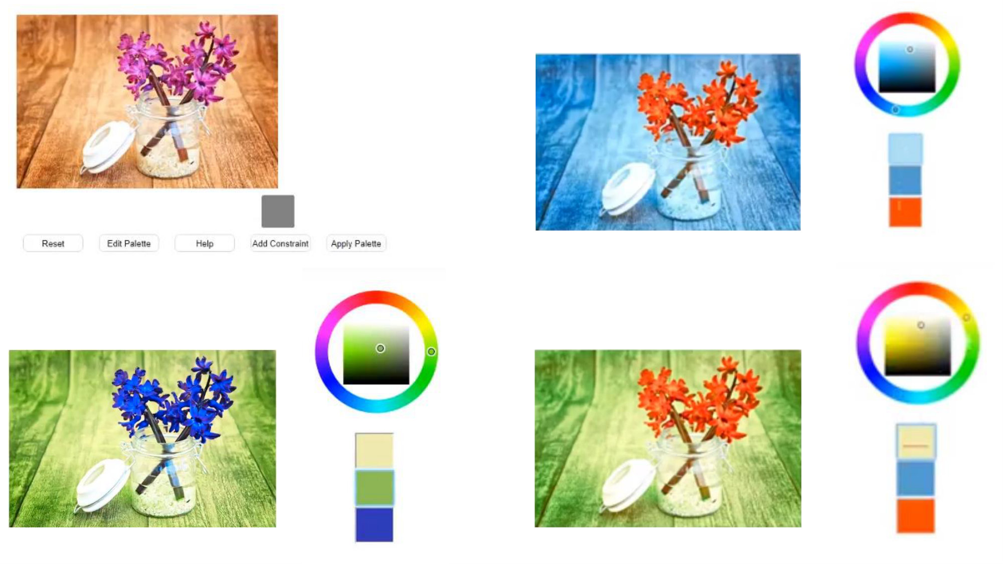 Figure 1
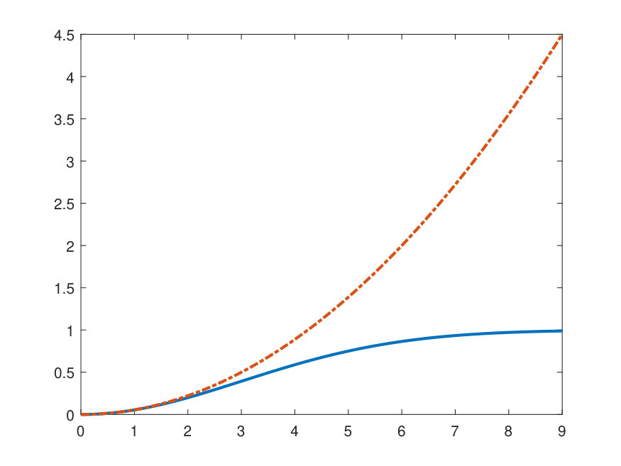 Figure 2
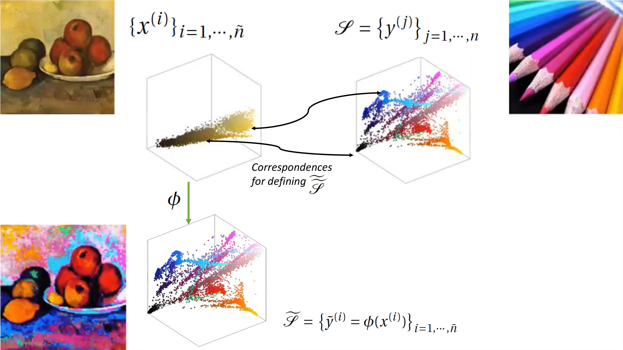 Figure 3
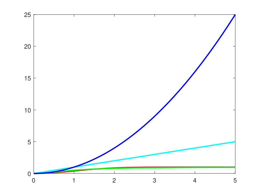 Figure 4
Peer Reviews
No public reviews on file for this paper yet. If you reviewed it on a platform where reviews are public (OpenReview, ICLR, NeurIPS, ICML), you can paste yours below so the community can read it here.
Videos
No videos yet. Explain this paper in a talk, walkthrough, or lecture? Add one.
Entropic Regularisation of Robust Optimal Transport
Rozenn Dahyot
School of Computer Science and Statistics
Trinity College Dublin, Ireland
[email protected], [email protected], [email protected]
Hana Alghamdi and Mairead Grogan
School of Computer Science and Statistics
Trinity College Dublin, Ireland
[email protected], [email protected], [email protected]
Abstract
Grogan et al. [11, 12] have recently proposed a solution to colour transfer by minimising the Euclidean distance between two probability density functions capturing the colour distributions of two images (palette and target). It was shown to be very competitive to alternative solutions based on Optimal Transport for colour transfer. We show that in fact Grogan et al’s formulation can also be understood as a new robust Optimal Transport based framework with entropy regularisation over marginals.
Keywords: M-estimation, estimator, Optimal Transport, Colour Transfer
1 Introduction
Optimal transport (OT) [16] has been successfully used as a way for defining cost functions for optimisation when performing colour transfer [17] and more recently in machine learning [4, 16]. The optimal transport cost (e.g Wasserstein distance) itself is also used as a similarity metric for retrieval [18]. For colour transfer (see Fig. 1111Images extracted from video https://youtu.be/FfrdyKMBVRc (demo for [12]) have been used for designing Fig. 1.), Grogan et al. [11, 12] have recently proposed an alternative approach for designing the cost function based on the divergence (see section 2). This based cost function is a weighted sum of multiple terms (terms in Eq. 1) able to take into account correspondences between images (via term in Eq. 1) when these are available, as well as the unsupervised scenario when no correspondence is available (via term in Eq. 1). In addition, includes entropies (terms and in Eq. 1). To further constrain the cost function when estimating the colour transformation , additional penalties can be added to prevent colours exceeding a certain range or forcing the estimated solution to be smooth (resp. terms and in Eq. 1). The estimate is computed as
[TABLE]
with:
[TABLE]
with indicating a normal distribution for random vector with expectation and covariance matrix . is the identity matrix, is a user defined bandwidth and are weights. This paper aims at proposing an OT formulation for the terms and (see Sec. 3) as an alternative to (presented in Sec. 2). In particular we show that these terms corresponds to robust Wasserstein distances where the bandwidth (Eq. 1) enables the seamless control of the level of robustness in a similar fashion as the scale parameter controlling M-estimators [13]. This reformulation allows the following contributions: first, to extend OT in supervised and semi-supervised scenarios, and second to propose a robust Wasserstein cost (Sec. 3). We start first by explaining in more detail the notations used and the cost function.
2 divergence
We consider that the following are available:
- •
a dataset : the term (Eq. 1) uses the samples from this dataset.
- •
a dataset computed using a transfer (or mapping) function on data points . The term (Eq. 1) uses the samples from this dataset.
- •
a dataset of correspondences : the term (Eq. 1) uses the samples from this dataset.
All data points have the same dimension (i.e. ) for any samples taken from , or . Figure 2 shows an illustration of our datasets in the context of colour transfer222Images from the video posted at https://twitter.com/gabrielpeyre/status/979605863295053826 have been used for designing Fig. 2..
In this framework [11], only one random vector (r.v.) is defined. Using and , two probability density functions noted and respectively are computed for r.v. as kernel density estimates with a Normal kernel (or Gaussian Mixture Models):
[TABLE]
and
[TABLE]
The unknown mapping function transforms the samples in that act as the means of the normal kernels in the mixture . Hence, can be warped onto by finding the appropriate function . The best choice for function can be chosen as minimising the Euclidean distance between and defined as [14]:
[TABLE]
from which terms in the cost function originate (Eq. 1). Such a formulation of has been used for colour transfer [11] and shape registration [14, 1]. The connection between with robust M-estimators has also been shown [3, 19, 14].
Removing from the cost function .
does not depends on and can be discarded, shortening into [19] for estimating . Both and correspond to entropies since and are the quadratic Renyi entropies of and respectively [11].
Using correspondences.
The term to account for correspondences in , is explained intuitively with notation by Grogan et al [12], where this time and are likewise kernel density estimates (with Normal kernel) using only observations in the dataset of correspondences :
[TABLE]
and the scalar product then corresponds to:
[TABLE]
Hence the notation is not mathematically correct to explain (i.e note the single sum for in Eq. 1 versus the double sum appearing in Eq. 3). So even if the intuition for is sound and proves to be efficient in practice against the state of the art techniques for colour transfer [12, 11], its origin cannot be explained mathematically with and we provide next a better explanation for based on Optimal Transport.
3 Optimal Transport
We propose to reformulate both and from an OT perspective. OT aims at choosing with the minimum transport (displacement) cost between two random vectors noted and . The OT cost function is expressed here with the Wasserstein distance [16] as follow:
[TABLE]
where is a cost often chosen as (quadratic Wasserstein distance), and is the joint probability density function of and having and for marginals respectively i.e. and . We first present our choices for these distributions (Sec. 3.1) and then propose a new robust cost (in Sec. 3.2). An alternative OT based explanation for terms and then emerges (Sec. 3.3).
3.1 Models for , and
Kernel density estimates with Normal kernels are used as joint density functions and using the datasets available, three estimates of can be proposed:
- •
using independent sets and (unsupervised scenario i.e without correspondences):
[TABLE]
with the marginals
[TABLE]
and
[TABLE]
- •
using the set of correspondences (supervised):
[TABLE]
providing the marginals
[TABLE]
and:
[TABLE]
- •
Using all datasets, the following mixture can be considered (semi-supervised):
[TABLE]
where is a parameter controlling the importance between the estimates and . In this case, the marginals are:
[TABLE]
and
[TABLE]
Note that these models noted are parameterized by via the samples in and . The bandwidths and are user defined and using enables the recovery of the empirical pdf estimates with Dirac kernels.
3.2 Robust cost
Concave functions to define costs of the form have been suggested for robustness [8]. Here, we go further by proposing the following robust cost:
[TABLE]
where is a constant that can be added if one need to enforce a positive cost . Our cost is convex near the origin and then becomes concave as the difference increases. We also note that:
[TABLE]
since integrates to 1 by definition. In practice, for estimation of that minimizes this cost, the constant does not matter and can be set .
3.2.1 Relation to M-estimators
With the more familiar notation for error , our robust cost is proportional to the Welsch-Leclerc loss [2]:
[TABLE]
which is a well-known hard redescending M-estimating function with scale parameter [13, 15, 7, 2]. The more the chosen function penalises large errors , the more it is robust to outliers. See for instance in Fig. 3(a) how the hard redescending functions (for Geman-McClure loss [6, 2]) and have an upper finite limit (equal to 1) when and thus prevent high residuals (outliers) to overly contribute too much when estimating . The non-robust Least Square function is also shown and corresponds here to the quadratic Wasserstein cost that is not robust to gross errors.
3.2.2 Relation of robust cost to Wasserstein distance
When the bandwidth (or scale parameter ) is very very large compared to , using Taylor approximation of the cost shows that (cf. Fig. 3(b)):
[TABLE]
making our cost proportional to the one used in the quadratic Wasserstein distance. The bandwidth allows for the modulation of the cost from the non robust Euclidean distance () to a more robust cost ( small) for penalising high differences (or outliers).
3.3 OT perspective for terms and
Using the definitions of our cost and our joint probability density functions (cf. Sec. 3.1), we note that:
[TABLE]
hence it is equivalent to the term (since the bandwidths are user defined). Likewise we note
[TABLE]
which is equivalent to (Eq. 1) introduced by Grogan et al to take advantage of correspondences [11]. Since the weight was chosen in an ad hoc fashion, we can propose a more elegant alternative form combining and into a new term using the estimate :
[TABLE]
With the OT formulation (Eq. 4), Grogan et al’s estimation (terms and , Eq. 1) can be rewritten:
[TABLE]
to which entropic terms on the marginals and ( and ) can be added along with other constraints on (e.g. and ).
When setting for simplicity (i.e. using empirical pdf estimates with Dirac kernels, Sec. 3.1), Grogan et al’s terms and are robust OT distances where the parameter in the robust cost controls the influence of outliers when performing estimation of the mapping function in the same way as the scale parameter for M-estimation.
3.4 Parametric Modelling of the transfer function
In practice, a parametric form of is used: Thin Plate Splines (TPS) have been used for colour transfer and shape registration [14, 11, 12]. The term in Eq. 1 corresponds to a smoothness constraint on the TPS solution [14, 11]:
[TABLE]
However TPS is not a convenient formulation when modelling transfer functions in high dimensional spaces and Deep Neural Networks are now providing more powerful formulations for .
3.5 Interpretation and Generalization of the cost
Our formulation of OT is equivalent to :
[TABLE]
where more generally can be understood as a conditional pdf ( given or vice versa since the Normal distribution is symmetric w.r.t. its mean). Using a flat prior for (e.g. with bandwidth very large to approximate a flat prior), then a model for the joint probability density function is available and our OT formulation (Eq. 17) is equivalent to:
[TABLE]
which has the same form as the cross product appearing in (cf. Eq. 2): as indicated in [11], the main difference between the two frameworks lies in the modelling of one r.v. ( in , with notation indicating integration over this one vector) or two r.v. ( and in OT, indicating integration over these two vectors). These scalar products between probability densities functions (joint, marginals or conditionals) are frequent for robust estimation including for instance the Hough transform widely used in image processing [5, 7, 9]. While some robust costs can be identified as a negative log likelihood [6, 2], we identify directly our robust cost as a negative Multivariate Normal distribution instead.
4 Final remarks
We have proposed a new generic formulation for Optimal Transport with the following advantages:
- •
it is robust: our new robust cost is parameterised by a bandwidth that acts like the scale parameter of M-estimators. This bandwidth enables the control of the level of robustness and when chosen very large, it makes our cost converge towards the standard (non robust) quadratic Wasserstein distance.
- •
Our formulation can seamlessly consider various scenarios e.g. unsupervised, supervised (with correspondences) or semi-supervised depending on the dataset(s) available.
- •
Grogan et al [11] propose the use of entropy terms for the marginals (e.g. ) that can be used in addition to (or instead of) an entropy on the joint pdf [16].
- •
More generally, we have shown the commonality of these formulations ( and OT) in using scalar products between two p.d.fs. The main difference between and OT is then in the number of random vectors used in the formulation of this scalar product. We believe this thinking extends to the Gromov-Wasserstein formulation which defines 4 random vectors [20].
Beyond the impact of our formulation for colour transfer [12, 11], future work will investigate shape registration with correspondences (e.g. for user interactions) and with kernels other than Gaussian better suited to directional data [10].
Acknowledgments
This work is partly supported by a scholarship from Umm Al-Qura University, Saudi Arabia, and in part by a research grants from Science Foundation Ireland (SFI) (Grant Number 15/RP/2776), and the ADAPT Centre for Digital Content Technology (www.adaptcentre.ie) that is funded under the SFI Research Centres Programme (Grant 13/RC/2106) and is co-funded under the European Regional Development Fund.
The reference list from the paper itself. Each links out to its DOI / PubMed record.
- 1[1] C. Arellano and R. Dahyot. Robust ellipse detection with gaussian mixture models. Pattern Recognition , 58:12 – 26, 2016.
- 2[2] J. T. Barron. A more general robust loss function. Co RR , abs/1701.03077, 2017.
- 3[3] A. Basu, I. R. Harris, N. L. Hjort, and M. C. Jones. Robust and efficient estimation by minimising a density power divergence. Biometrika , 85(3):549–559, 1998.
- 4[4] N. Courty, R. Flamary, D. Tuia, and A. Rakotomamonjy. Optimal transport for domain adaptation. IEEE Transactions on Pattern Analysis and Machine Intelligence , 39(9):1853–1865, Sep. 2017.
- 5[5] R. Dahyot. Statistical hough transform. IEEE Transactions on Pattern Analysis and Machine Intelligence , 31(8):1502–1509, Aug 2009.
- 6[6] R. Dahyot, P. Charbonnier, and F. Heitz. A bayesian approach to object detection using probabilistic appearance-based models. Pattern Analysis and Applications , 7(3):317–332, Dec 2004.
- 7[7] R. Dahyot and J. Ruttle. Generalised relaxed radon transform (gr 2t) for robust inference. Pattern Recognition , 46(3):788 – 794, 2013.
- 8[8] J. Delon, J. Salomon, and A. Sobolevski. Local matching indicators for transport problems with concave costs. SIAM Journal on Discrete Mathematics , 26(2):801–827, 2012.