Dissipative periodic and chaotic patterns to the KdV--Burgers and Gardner equations
Stefan C. Mancas, Ronald Adams

TL;DR
This paper analyzes the dynamics of the KdV-Burgers and Gardner equations with dissipation and external perturbations, revealing bifurcations, stability changes, and chaotic behavior through dynamical systems and Shil'nikov's analysis.
Contribution
It introduces a reduced two-parameter dynamical system to study bifurcations and chaos in the KdV-Burgers and Gardner equations, including the application of Shil'nikov's theorem.
Findings
Hopf bifurcation leads to stable limit cycles
Homoclinic chaos observed in KdV-Burgers case
Stable periodic orbits in Gardner equation
Abstract
We investigate the KdV-Burgers and Gardner equations with dissipation and external perturbation terms by the approach of dynamical systems and Shil'nikov's analysis. The stability of the equilibrium point is considered, and Hopf bifurcations are investigated after a certain scaling that reduces the parameter space of a three-mode dynamical system which now depends only on two parameters. The Hopf curve divides the two-dimensional space into two regions. On the left region the equilibrium point is stable leading to dissapative periodic orbits. While changing the bifurcation parameter given by the velocity of the traveling waves, the equilibrium point becomes unstable and a unique stable limit cycle bifurcates from the origin. This limit cycle is the result of a supercritical Hopf bifurcation which is proved using the Lyapunov coefficient together with the Routh-Hurwitz criterion. On the…
Click any figure to enlarge with its caption.
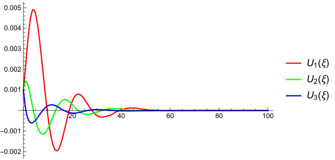 Figure 1
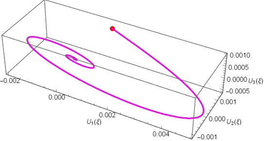 Figure 2
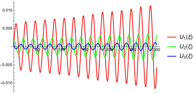 Figure 3
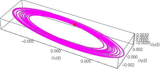 Figure 4
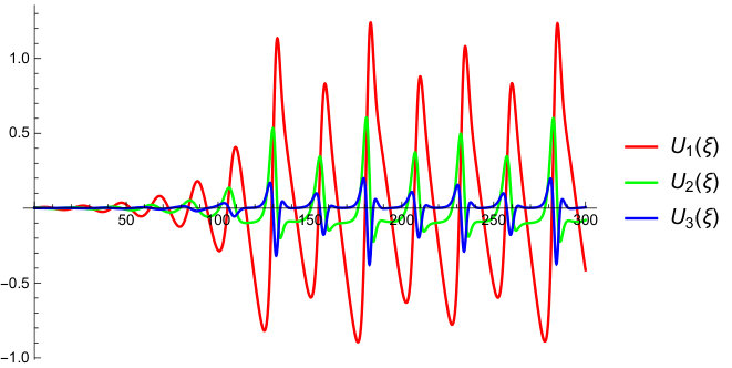 Figure 5
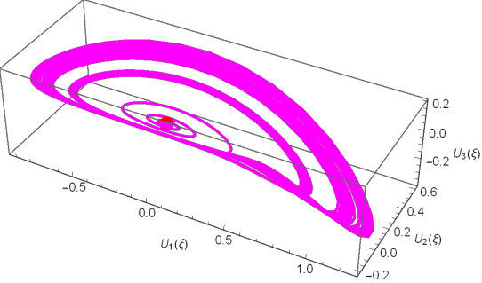 Figure 6
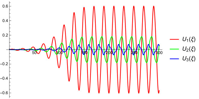 Figure 7
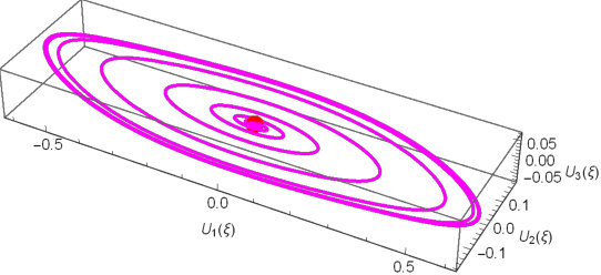 Figure 8
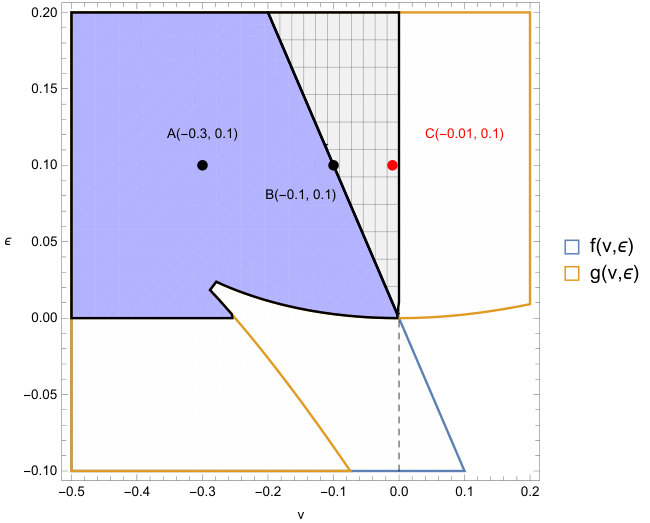 Figure 9
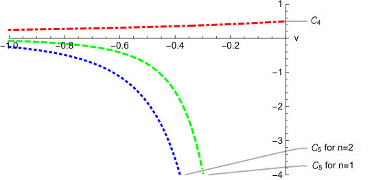 Figure 10
 Figure 11
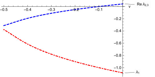 Figure 12
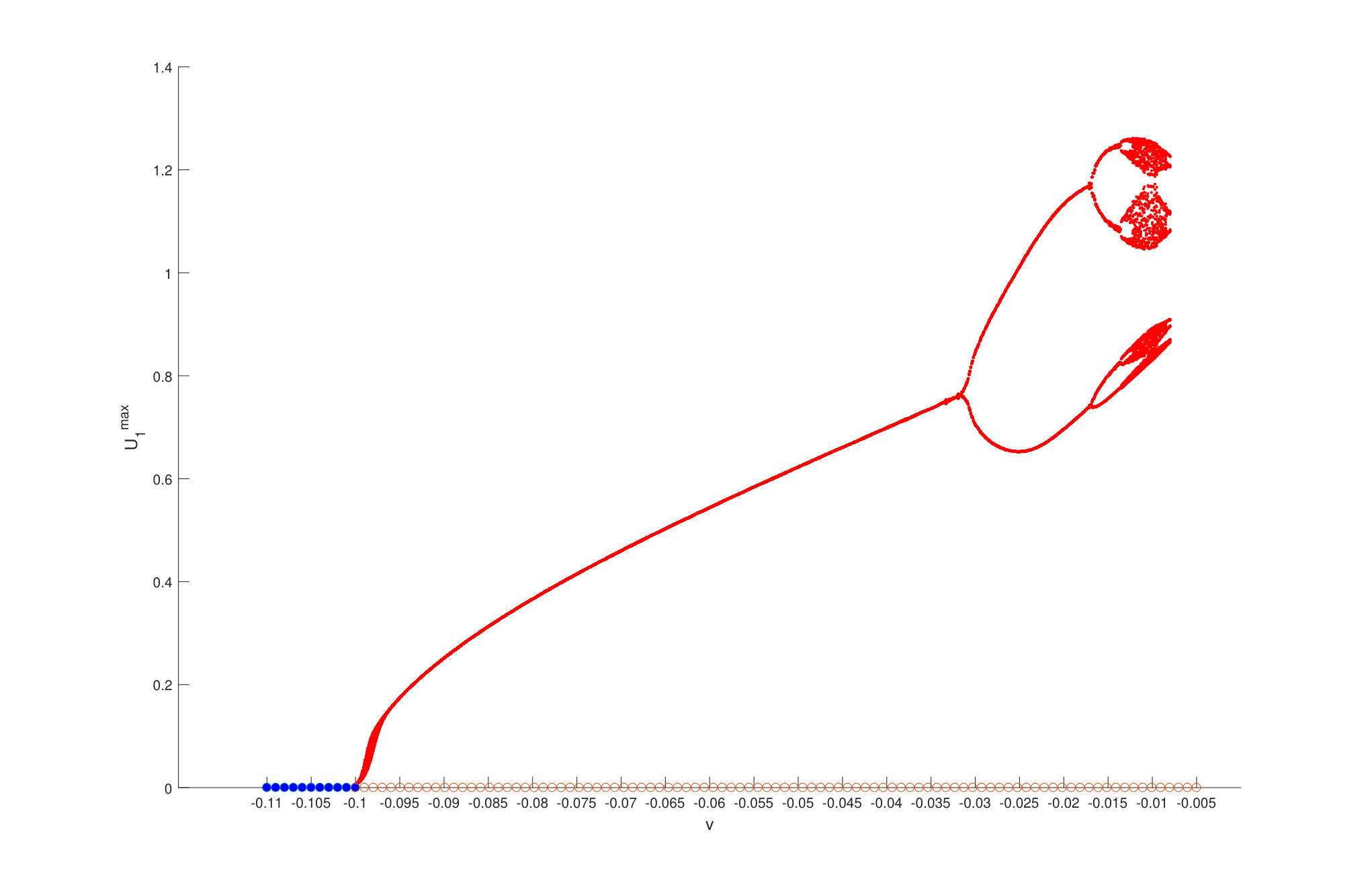 Figure 13
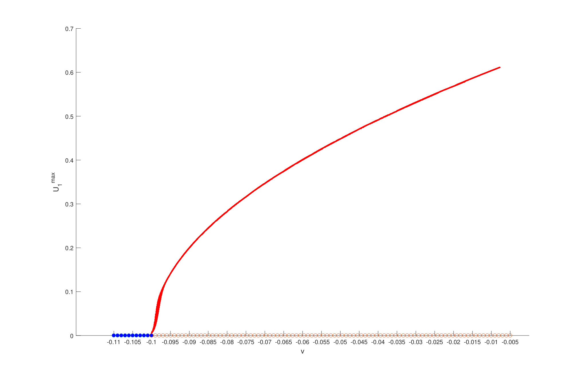 Figure 14
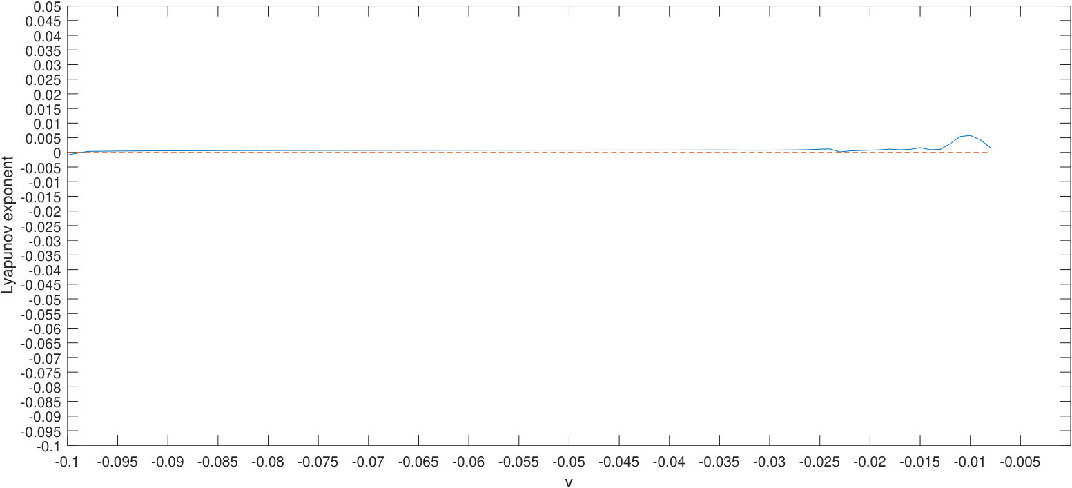 Figure 15
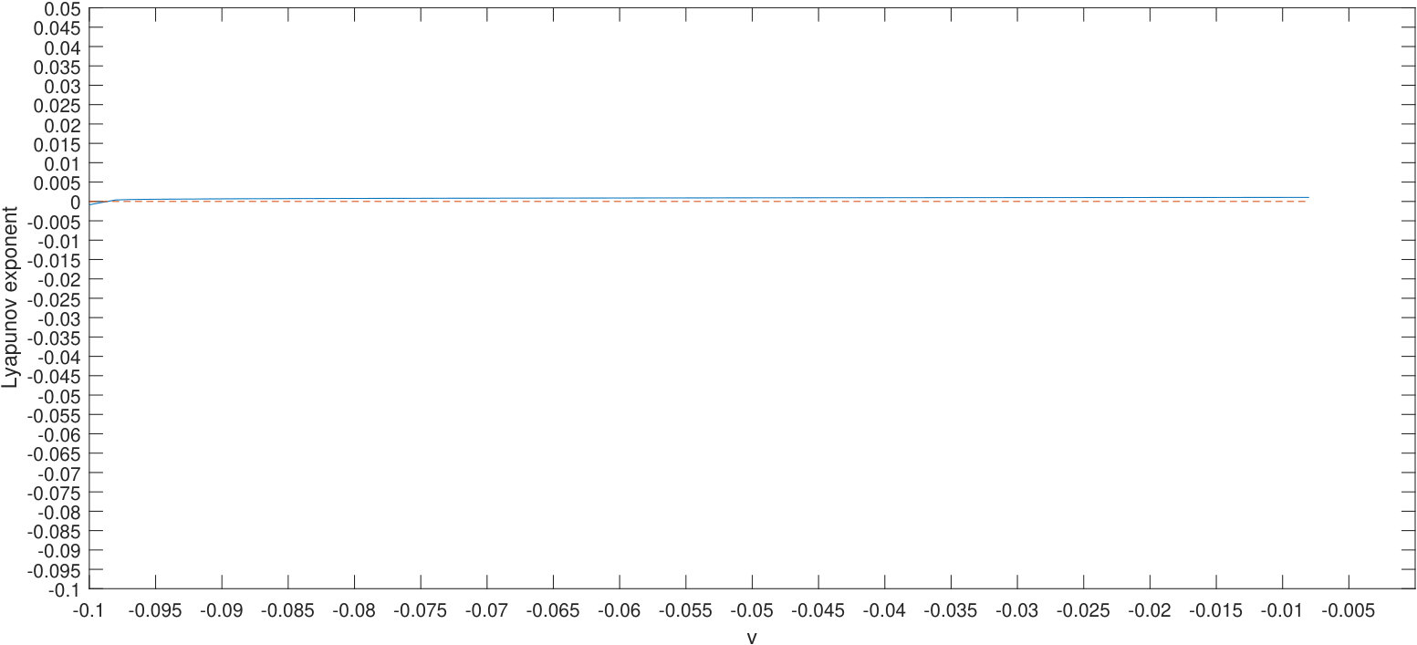 Figure 16
Peer Reviews
No public reviews on file for this paper yet. If you reviewed it on a platform where reviews are public (OpenReview, ICLR, NeurIPS, ICML), you can paste yours below so the community can read it here.
Videos
No videos yet. Explain this paper in a talk, walkthrough, or lecture? Add one.
Dissipative periodic and chaotic patterns to the
KdV–Burgers and Gardner equations
Stefan C. Mancas
Department of Mathematics, Embry-Riddle Aeronautical University
Daytona Beach, FL 32114-3900, USA
Ronald Adams
Department of Mathematics, Embry-Riddle Aeronautical University
Daytona Beach, FL 32114-3900, USA
Abstract
We investigate the KdV-Burgers and Gardner equations with dissipation and external perturbation terms by the approach of dynamical systems and Shil’nikov’s analysis. The stability of the equilibrium point is considered, and Hopf bifurcations are investigated after a certain scaling that reduces the parameter space of a three-mode dynamical system which now depends only on two parameters. The Hopf curve divides the two-dimensional space into two regions. On the left region the equilibrium point is stable leading to dissapative periodic orbits. While changing the bifurcation parameter given by the velocity of the traveling waves, the equilibrium point becomes unstable and a unique stable limit cycle bifurcates from the origin. This limit cycle is the result of a supercritical Hopf bifurcation which is proved using the Lyapunov coefficient together with the Routh-Hurwitz criterion. On the right side of the Hopf curve, in the case of the KdV-Burgers, we find homoclinic chaos by using Shil’nikov’s theorem which requires the construction of a homoclinic orbit, while for the Gardner equation the supercritical Hopf bifurcation leads only to a stable periodic orbit.
Keywords: KdV-Burgers, Gardner, Hopf bifurcation, Shil’nikov’s analysis, Lyapunov, homoclinic orbit, chaos.
I Introduction
We consider the nonlinear evolution equation
[TABLE]
for which the case represents the KdV-Burgers equation KdVB , while corresponds to the Gardner equation (sometimes known as the modified KdV-Burgers), which is the equation for nonlinear dissipative waves in solid wave guides Gard . The terms that contain the and coefficients take an account the effects of dissipation and an external linear perturbation, and are imperative for leading to chaos. Such additional terms appear in non-uniform plasmas in the form of viscous or collisional effects, and they have been introduced as a perturbation of the KdV equation by Allen and Rowlands Allen , where they have found the form and speed of a new solitary-wave solution to the perturbed KdV equation that depends on two parameters. The case has been discussed by Karpman and Maslov where they found that the original soliton changes speed and shape, and forms a long tail at the end of which there are small oscillations in time and spaceKarp . In Chang et al. the authors analyzed the behavior of an ion-acoustic soliton as it propagates from a high density to a low density region Chang , while Kivshar and Malomed Kiv utilized the inverse scattering technique to establish the evolution of the single soliton solution in the presence of perturbations. Exact solutions to (1) when and have been obtained using the factorization method by Cornejo-Pérez and collaborators Har .
In this paper we discuss the case where both coefficients and , and note that and may be set to unity by using the scaling with , and . For , , , one obtains the non-dimensional equation
[TABLE]
with Employing the traveling wave ansatz , where is the traveling wave variable, v is translational speed of waves traveling in the positive direction at time , and is a bifurcation parameter, then (2) becomes
[TABLE]
As a three-mode dynamical system (3) takes the compact form
[TABLE]
where , , is the Jacobian matrix, and .
II Linear stability analysis
Following standard methods of phase-plane analysis the equilibrium point P_{0}\big{(}U_{1}(\xi_{0}),U_{2}(\xi_{0}),U_{3}(\xi_{0})\big{)} of (4) is the origin, and the characteristic polynomial of the Jacobian matrix at is given by the cubic polynomial
[TABLE]
where , and . By the Routh-Hurwitz criteria Hurwitz ; Routh the necessary and sufficient condition for the stability of the equilibrium point is that all eigenvalues of (5) must have negative real parts, which implies
[TABLE]
On the contrary, one may have the onset of instability of the solution occurring in one of two ways Mancas . First, the equilibrium becomes non-hyperbolic due to one of the eigenvalues crossing through the origin and would occur when
[TABLE]
which is known as the static instability. However, this condition cannot be achieved since . Second, the dynamic instability condition occurs when a pair of eigenvalues of the Jacobian become purely imaginary. The consequent Hopf bifurcation curve is given by
[TABLE]
and leads to periodic solutions of (4) which dissipate by slowly converging to the origin. These solutions, denoted by and may be asymptotic to the origin or to a limit cycle depending on the super- or subcritical nature of the bifurcation, and in general are quasi-periodic wavetrains, since their periods are typically incommensurate Mancas .
To find the eigenvalues of the Jacobian matrix, we shift the eigenvalue according to to obtain the depressed cubic
[TABLE]
with coefficients and . By using Cardano’s formula Car , we define
[TABLE]
where the modular discriminant is . For a real non-repeated eigenvalue and a complex conjugate pair, we require the additional condition
[TABLE]
which gives the eigenvalues
[TABLE]
This condition leads to the elliptic curve inequality
[TABLE]
where we set .
We summarize all these conditions as follows:
- i)
the Hopf bifurcation curve is given by
[TABLE]
and leads to periodic solutions, 2. ii)
for stability we require that holds which gives
[TABLE] 3. iii)
using we also require that .
All these three conditions combined depict the dark shaded region of Fig. 1.
For a supercritical Hopf bifurcation the complex eigenvalues cross the imaginary axis into the right half plane, and the Lyapunov coefficient calculated using (18) is negative. On the boundary of stability the eigenvalues are , and for . These eigenvalues determine a factorization of the characteristic polynomial (5) as
[TABLE]
which leads to , , and . The last two relations give the condition , and using (12), on the Hopf curve we have
[TABLE]
which gives the solutions , and .
Now we will perturb the manifold by a small velocity , such that . Thus, if we are located on the right side of , while if , we are on the left. Returning to the complex eigenvalues we have , with and on which gives . Along this codimension-one manifold we consider the following non-degeneracy conditions:
- (A1):
- (A2): , which is the first Lyapunov coefficient given by (18).
To verify (A1) we compute , and we have
[TABLE]
where .
To verify (A2) we now need to determine which is dependent on the Taylor expansion of about . This can be written up to order four as , where and are multilinear vector functions with components defined by the vectors and are given by
[TABLE]
for . Along the curve , has a pair of purely imaginary eigenvalues with corresponding eigenvectors such that . Writing these values in terms of v as , we have the eigenvectors
[TABLE]
Let be the corresponding adjoint eigenvector such that , and since we require that , then
[TABLE]
Now, we can then determine the expression for as given by Kuznetsov Kuz , which is
[TABLE]
where is the identity matrix. This expression depends on and which also depend on .
For we have
[TABLE]
while is zero, and by using (18) the Lyapunov coefficient is
[TABLE] 2. 2.
For we have
[TABLE]
while is zero, and using (18) gives
[TABLE]
The non-degeneracy conditions (A1) and (A2) hold along the curve since and for , see Fig. 2. Thus, in both cases and , (4) undergoes a supercritical Hopf bifurcation, and hence a unique stable limit cycle bifurcates from the origin.
Now that we have established that (4) undergoes a supercritical Hopf bifurcation, we turn our attention to specific points in the parameter space of Fig. 1 which will uncover further qualitative properties of the solutions to (4). For a fixed , on the left of the Hopf curve ( for the equilibrium point shown as solid circles in the bifurcation diagrams of Figs. 3 and 4 is asymptotically stable, while the open circles in the same figures indicate that the equilibrium point is unstable. For case A when , the dissipative periodic orbit is shown in Fig. 9 of the Appendix. Because case A is located to the left of the Hopf curve, the solution converges asymptotically to the origin. On the Hopf curve , the origin becomes weakly stable, this is witnessed by considering case B and the corresponding solution in Fig. 10 of the Appendix. Passing to the right of the Hopf curve for , the origin becomes unstable and a stable limit cycle exists for case C. When this limit cycle undergoes a period doubling bifurcation, see Fig. 3, and the formation of limit cycles of period two, four, eight, etc. are created which is a classic signature of chaos. The limit cycle in this case is a chaotical attractor which will be confirmed using Shil’nikov’s analysis in the following section. Whereas for a unique stable limit cycle is produced see Fig. 4, and no chaos is observed. We compute numerically the solutions for case C, for both and resepctively. The solution which tends towards a chaotical attractor for is shown in Fig. 11, while for , the solution which tends to a stable periodic orbit is shown in Fig. 12 of the Appendix.
Next, we compute numerically the maximal Lyapunov exponent for for both and by using the algorithm detailed in wolf , which measures the degree of sensitivity to initial conditions.
When , we can infer from Fig. 5 that as the Hopf curve is transversed in the v direction at the equilibrium becomes a saddle-focus and eventually the system experiences chaotic dynamics which is due to a period doubling bifurcation. The graph of the largest Lyapunov exponent is positive for v around and gives us a parameter range for selecting candidate values of v when applying the Shil’nikov criteria. In this region the phase portraits near the limit cycle have an infinite number of saddle cycles which correspond to periodic wavetrains of (4). The limit cycle has an oscillating tail, while secondary limit cycles near the saddle-focus homoclinic bifurcation correspond to double traveling impulses of (4). This is synonymous with deterministic chaos provided the corresponding unstable manifold folds back onto itself and remains confined within a bounded domain which confirms the existence of periodic and chaotic trajectories for KdV-Burgers equation.
When , Fig. 6 indicates a close to zero Lyapunov exponent, that is, no sensitivity to initial conditions. This combined with the bifurcation diagram of Fig. 4 leads us to conclude that there is no chaos present for (4) in the case of Gardner equation.
III Shil’nikov’s analysis of homoclinic orbits
In this section, the algebraic expression of the homoclinic orbit is derived for in (4), and the uniform convergence of its series expansion is proved. In particular, the Shil’nikov criterion Roy is verified by applying Shil’nikov’s theorem (Theorem 2.1 in Sil ), and thus ensuring that the system (4) is chaotic. We fix starting from the initial condition , and we vary the bifurcation parameter v. As observed in Fig. 3, a period doubling route to chaos is present for . In order to carry out the Shil’nikov analysis, the conditions (B1), (B2) together with the existence of a homoclinic orbit which defines a traveling impulse must be established. These conditions are:
- (B1): ,
- (B2): (the Shil’nikov inequality).
Let us first consider (B1), for , and , which is a region to the right of () depicted by the meshed area in Fig. 1 where point C is located. Since we can explicitly compute . From Fig. 7, we see that to the right of the Hopf curve the origin becomes a saddle focus, therefore (B1) is satisfied. For (B2) we have the following relation between eigenvalues: , therefore (B2) can be expressed as . This inequality is easily verified when . On the other hand if , then we have . As we can see from Fig. 8 this is valid for and .
We now discuss the existence of a non-trivial homoclinic orbit of (4) connecting the origin to itself, that is, a trajectory of (4) (not restricted to the origin) which is doubly asymptotic to the origin. We use the parameter values given by case C to construct the homoclinic orbit, but the procedure carried out below can be adapted for other parameter regimes as well.
Theorem III.1**.**
If and (B1), (B2) are satisfied, then system (4) has one homoclinic orbit whose first component has the form (21), and the corresponding chaos is of horseshoe type.
Proof. We start by assuming a solution to (3) is in the form
[TABLE]
for , where is an undetermined constant with . From (3) with we have the following relation
[TABLE]
Comparing the coefficients of in (22) of the same power terms for we obtain
[TABLE]
which is equivalent to . In the meshed region of Fig. 1, where point C is located, and where the condition (B1) is satisfied we know that , therefore a unique negative root of is determined by the real eigenvalue in (12). Notice that in this region the two other roots have positive real parts, see Fig. 8. Hence we restrict our analysis to since using any of the other two eigenvalues would lead to a divergent series.
To retrieve asymptotically the non-trivial homoclinic orbit we must assume that in (21) , otherwise when then for all . Now if , for we have the following values
[TABLE]
In general for we have the recursive formula
[TABLE]
[TABLE]
where
[TABLE]
From (26) we see that the coefficients can be written in the closed form
[TABLE]
where the ’s can be computed by induction on and can be seen as functions depending upon , v, and .
To find the expression of for we assume that
[TABLE]
As in the case , we have
[TABLE]
where the ’s are some other functions that also depend on , v, and and satisfy . If then
[TABLE]
In order to construct a component of the homoclinic orbit we must impose the following smoothness conditions
[TABLE]
Hence, the component of the homoclinic orbit takes the form
[TABLE]
To determine numerically we use (35) which implies that . This can be solved using Newton’s method by using the corresponding truncated polynomial given by
[TABLE]
Using , we find , and since for large, this excludes the possibility that is a multiple root. Since is known, we can find using (30).
We seek to show that the series expansion in (35) converges absolutely, for this we use a series expansion argument as outlined in Zhou . We use the parameters of point C given by and . For other parameter regimes the proof is similar. Based on the values of and along with (26) we claim that
[TABLE]
for , for some . For the aforementioned values of and v we use Cardano’s formula (12) to determine . Next we compute by utilizing (27) in conjunction with (37), which gives the inequality
[TABLE]
For , we have the inequality
[TABLE]
This estimate is established by induction. Using (26) and the induction hypothesis (37), we have
[TABLE]
Since
[TABLE]
then
[TABLE]
Now, we can prove the convergence of the series
[TABLE]
The above estimate holds for all , thus, the series expansion (21) is uniformly convergent for all . The above argument can be duplicated for the case , therefore (35) is well defined.
IV Conclusion
A rigorous treatment of Hopf bifurcation analysis has been presented for the KdV-Burgers equation for and the Gardner equation for , with dissipative and perturbation terms. For both equations, left moving traveling waves are stable for and of the same sign. For a certain region of space the solutions undergo a supercritical Hopf bifurcation as the wave speed v crosses the Hopf curve when consequently a stable limit cycle is born for . For the KdV-Burgers equation the stable limit cycle undergoes a period doubling bifurcation indicating the existence of a Smale horseshoe. This is verified by applying the Shil’nikov criterion. By utilizing the undetermined coefficient method, a homoclinic orbit is identified and explicit and convergent algebraic expressions are derived. We show a parameter regime for when the system (4) has a homoclinic orbit of Shil’nikov type which implies horseshoe chaos, while for in the same parameter space the supercritical Hopf bifurcation leads only to stable periodic orbits. For both equations, right traveling waves for which correspond to dissipation and perturbation terms of opposite sign are unstable.
Appendix
References
- (1) Allen, M. A., and Rowlands, G. (2000). A solitary-wave solution to a perturbed KdV equation. Journal of Plasma Physics, 64(4), 475-480.
- (2) Burgers, J. M. (1948). A mathematical model illustrating the theory of turbulence. In Advances in Applied Mechanics (Vol. 1, pp. 171-199). Elsevier.
- (3) Chang, H. Y., Raychaudhuri, S., Hill, J., Tsikis, E. K., and Lonngren, K. E. (1986). Propagation of an ion‐acoustic soliton in an inhomogeneous plasma. The Physics of Fluids, 29(1), 294-297.
- (4) Gardner, C. S., Greene, J. M., Kruskal, M. D., and Miura, R. M. (1974). Korteweg de Vries equation and generalizations. VI. Methods for exact solution. Communications on Pure and Applied Mathematics, 27(1), 97-133.
- (5) Hurwitz, A. (1895). On the conditions under which an equation possesses only roots with negative real parts. Mathematical Annals, 46 (2), 273-284.
- (6) Karpman, V. I., and Maslov, E. M. (1978). Structure of tails produced under the action of perturbations on solitons. Soviet Journal of Experimental and Theoretical Physics, 48, 252.
- (7) Kivshar, Y. S., and Malomed, B. A. (1989). Dynamics of solitons in nearly integrable systems. Reviews of Modern Physics, 61(4), 763.
- (8) Kuznetsov, Y. A. (1998). Elements of Applied Bifurcation Theory (Vol. 112), Applied Mathematical Sciences(Springer-Verlag).
- (9) Mancas, S. C., and Choudhury, S. R. (2007). The complex cubic–quintic Ginzburg–Landau equation: Hopf bifurcations yielding traveling waves. Mathematics and Computers in Simulation, 74(4-5), 281-291.
- (10) Murray, J. D. (2002). Mathematical Biology. I, Vol. 17 of Interdisciplinary Applied Mathematics.
- (11) Cornejo-Pérez, O., Negro, J., Nieto, L. M., and Rosu, H. C. (2006). Traveling-wave solutions for Korteweg–de Vries–Burgers equations through factorizations. Foundations of Physics, 36(10), 1587-1599.
- (12) Routh, E. J. (1877). A treatise on the stability of a given state of motion: particularly steady motion. Macmillan and Company.
- (13) Silva. C. P., (1993). Shil’nikov’s theorem-a tutorial. IEEE Transactions on Circuits and Systems I: Fundamental Theory and Applications, 40(10), 675-682.
- (14) Spiegel, M. R., and Liu, J. (1999). Schaum’s mathematical handbook of formulas and tables (Vol. 1000). New York: McGraw-Hill.
- (15) Wolf, A., Swift, J. B., Swinney, H. L., and Vastano, J. A. (1985). Determining Lyapunov exponents from a time series. Physica D: Nonlinear Phenomena, 16(3), 285-317.
- (16) Van Gorder, R. A., and Choudhury, S. R. (2011). Shil’nikov Analysis of Homoclinic and Heteroclinic Orbits of the T System. Journal of Computational and Nonlinear Dynamics, 6(2), 021013.
- (17) Zhou, T., Tang, Y., and Chen, G. (2004). Chen’s attractor exists. International Journal of Bifurcation and Chaos, 14(09), 3167-3177.
The reference list from the paper itself. Each links out to its DOI / PubMed record.
- 1(1) Allen, M. A., and Rowlands, G. (2000). A solitary-wave solution to a perturbed Kd V equation. Journal of Plasma Physics, 64(4), 475-480.
- 2(2) Burgers, J. M. (1948). A mathematical model illustrating the theory of turbulence. In Advances in Applied Mechanics (Vol. 1, pp. 171-199). Elsevier.
- 3(3) Chang, H. Y., Raychaudhuri, S., Hill, J., Tsikis, E. K., and Lonngren, K. E. (1986). Propagation of an ion‐acoustic soliton in an inhomogeneous plasma. The Physics of Fluids, 29(1), 294-297.
- 4(4) Gardner, C. S., Greene, J. M., Kruskal, M. D., and Miura, R. M. (1974). Korteweg de Vries equation and generalizations. VI. Methods for exact solution. Communications on Pure and Applied Mathematics, 27(1), 97-133.
- 5(5) Hurwitz, A. (1895). On the conditions under which an equation possesses only roots with negative real parts. Mathematical Annals, 46 (2), 273-284.
- 6(6) Karpman, V. I., and Maslov, E. M. (1978). Structure of tails produced under the action of perturbations on solitons. Soviet Journal of Experimental and Theoretical Physics, 48, 252.
- 7(7) Kivshar, Y. S., and Malomed, B. A. (1989). Dynamics of solitons in nearly integrable systems. Reviews of Modern Physics, 61(4), 763.
- 8(8) Kuznetsov, Y. A. (1998). Elements of Applied Bifurcation Theory (Vol. 112), Applied Mathematical Sciences(Springer-Verlag).