Limiting absorption principle on Riemannian scattering (asymptotically conic) spaces, a Lagrangian approach
Andras Vasy

TL;DR
This paper establishes the limiting absorption principle on asymptotically conic Riemannian spaces using a Lagrangian framework, demonstrating Fredholm properties of spectral families in specialized function spaces.
Contribution
It introduces a Lagrangian approach to prove the limiting absorption principle on asymptotically conic spaces, extending scattering theory techniques.
Findings
Spectral family is Fredholm in Lagrangian-regularity spaces
Results hold for non-zero spectral parameters on and off the spectrum
Persistence of properties in the physical half plane
Abstract
We use a Lagrangian perspective to show the limiting absorption principle on Riemannian scattering, i.e. asymptotically conic, spaces, and their generalizations. More precisely we show that, for non-zero spectral parameter, the `on spectrum', as well as the `off-spectrum', spectral family is Fredholm in function spaces which encode the Lagrangian regularity of generalizations of `outgoing spherical waves' of scattering theory, and indeed this persists in the `physical half plane'.
Click any figure to enlarge with its caption.
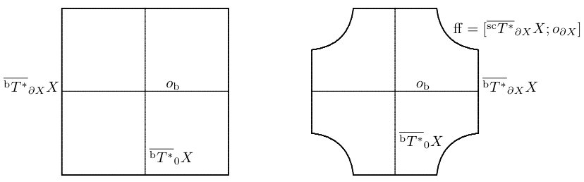 Figure 1
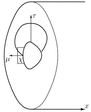 Figure 2
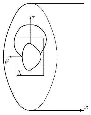 Figure 3
 Figure 4
Peer Reviews
No public reviews on file for this paper yet. If you reviewed it on a platform where reviews are public (OpenReview, ICLR, NeurIPS, ICML), you can paste yours below so the community can read it here.
Videos
No videos yet. Explain this paper in a talk, walkthrough, or lecture? Add one.
Limiting
absorption principle on Riemannian scattering (asymptotically conic) spaces, a Lagrangian approach
András Vasy
Department of Mathematics, Stanford University, CA 94305-2125, USA
(Date: . Original version: May 29, 2019)
Abstract.
We use a Lagrangian perspective to show the limiting absorption principle on Riemannian scattering, i.e. asymptotically conic, spaces, and their generalizations. More precisely we show that, for non-zero spectral parameter, the ‘on spectrum’, as well as the ‘off-spectrum’, spectral family is Fredholm in function spaces which encode the Lagrangian regularity of generalizations of ‘outgoing spherical waves’ of scattering theory, and indeed this persists in the ‘physical half plane’.
2000 Mathematics Subject Classification:
Primary 35P25; Secondary 58J50, 58J40, 35P25, 35L05, 58J47
The author gratefully acknowledges partial support from the NSF under grant numbers DMS-1361432 and DMS-1664683 and from a Simons Fellowship.
1. Introduction and outline
The purpose of this paper is to prove the limiting absorption principle, concerning the limit of the resolvent at the spectrum on appropriate function spaces, for Laplace-like operators on Riemannian scattering (asymptotically conic at infinity) spaces using a description that focuses on the outgoing radial set, which in phase space corresponds to the well-known outgoing spherical waves in Euclidean scattering theory. Thus, the result is a precise description of the limiting resolvent in terms of mapping properties on spaces of (finite regularity) Lagrangian distributions, where now the Lagrangian is conic in the base manifold, rather than the fibers of the cotangent bundle as familiar from standard microlocal analysis. Such a result is well suited for the analysis of waves, especially at the ‘radiation face’, or ‘scri’, see [5], though we do not pursue this aspect here. We explain more of the historic context of Lagrangian analysis in scattering theory below, but already remark that recently such a Lagrangian analysis proved very effective in the description of internal waves in fluids by Dyatlov and Zworski [2].
The basic setting is Melrose’s scattering pseudodifferential algebra , see [11], which for the radial compactification of (to a ball) goes back to Parenti and Shubin [14, 15], and which corresponds to any standard quantization of symbols with the property
[TABLE]
with the decay order and the differential order. The key property of this algebra is that the principal symbol is taken modulo better terms, thus also captures decay at infinity; see Section 2 for more detail.
With this in mind, recall first that for real, elements of the spectral family are not elliptic in this algebra due to the part of the principal symbol capturing decay (essentially as can vanish), rather have a non-degenerate real principal symbol with a source-to-sink Hamilton flow within their characteristic set (the zero set of the principal symbol). One obtains a Fredholm problem using variable decay order weighted scattering Sobolev spaces (which are the standard Sobolev space on , albeit of a microlocally variable order), where the order only matters on the characteristic set, needs to be monotone along the Hamilton flow, and be greater than a threshold value ( in the standard case, for the domain of the operator; the target space has one additional order of decay) for one of the radial sets (source or sink), which we call the incoming one, and less than a threshold value for the other one, which we call the outgoing one, see [21], and see also [3] for a semiclassical version in a dynamical systems setting. Moreover, this gives the limiting absorption resolvent where the vs. limits (in terms of the spectral parameter , thus shows that corresponds to the limit if , and the limit if ) correspond to propagating estimates forward along the Hamilton flow, i.e. having high decay order at the source, vs. propagating estimates backwards, i.e. having high decay order at the sink. This can then be extended uniformly to zero energy, see [22], using second microlocal methods discussed below.
A different way of arranging a Fredholm setup is by considering a fixed decay order Sobolev space which is lower than the threshold order, but adding to it extra Lagrangian regularity relative to elements of characteristic on the outgoing radial set (referred to as ‘module regularity’, see [6, 7, 4], see also [2]). (Since the Lagrangian is at finite points in the fibers of the scattering cotangent bundle, i.e. where is finite in the Euclidean picture, the differential order is immaterial; only the decay order matters.) For instance, the background decay order can be taken less than the threshold, and one may require regularity under one such pseudodifferential factor. This makes the space to have order more decay everywhere except at the outgoing radial set; since the thresholds are the same in this case at both radial sets, this means that we have higher order decay at the incoming radial set than the threshold. Very concretely, this can be arranged using operators
[TABLE]
with the boundary defining function, local coordinates on the boundary, and the metric is to leading order warped product type relative to these. (So in the asymptotically Euclidean setting, one could have , and local coordinates on the sphere with respect to the standard spherical coordinate decomposition.) Thus, the domain space is the modified version of
[TABLE]
with the modification just so that the operator maps it to the target which simply has additional order of decay
[TABLE]
Using the variable order Fredholm theory it is straightforward to show (using a variable order that is in at the incoming radial set, and is at the outgoing radial set) that the outgoing inverse indeed has the property that under this additional regularity of the input (in the target space), the output lies in the additional regularity domain. However, it is harder to directly run Fredholm arguments since these involve duality and inversion, and the additional module regularity gives a dual space for which it is harder to prove estimates since the dual of, for instance, the space (1.1) is
[TABLE]
see [12, Appendix A].
A way around this difficulty with dualization, which we pursue in this paper, is to use even stronger, second microlocal, spaces, see [22, Section 5] in this scattering context, and see [1, 16, 19] in different contexts. Recall that these second microlocal techniques play a role in precise analysis at a Lagrangian, or more generally coisotropic, submanifold. These second microlocal techniques were employed in [22] due to the degeneration of the principal symbol at zero energy, corresponding to the quadratic vanishing of any dual metric function at the zero section; the chosen Lagrangian is thus the zero section, really understood as the zero section at infinity. In a somewhat simpler way than in other cases, this second microlocalization at the zero section is accomplished by simply using the b-pseudodifferential operator algebra of Melrose [13]. In an informal way, this arises by blowing up the zero section of the scattering cotangent bundle at the boundary, though a more precise description (in that it makes sense even at the level of quantization, the spaces themselves are naturally diffeomorphic) is the reverse: blowing up the corner (fiber infinity over the boundary) of the b-cotangent bundle: see Section 2 for more detail and additional references. (But the basic point is that the scattering vector fields are replaced by totally characteristic, or b-, vector fields .) In [22] this was used to show a uniform version of the resolvent estimates down to zero energy using variable differential order b-pseudodifferential operators. Indeed, the differential order of these, cf. the aforementioned blow-up of the corner, corresponds to the scattering decay order away from the zero section, thus this allows the uniform analysis of the problem to zero energy. However, here the decay order (of the b-ps.d.o.) is also crucial, for it corresponds to the spaces on which the exact zero energy operator (i.e. with ) is Fredholm, which, with denoting weighted b-Sobolev spaces relative to the scattering (metric) -density, are with , where is the variable order (which is irrelevant at zero energy since the operator is elliptic in the b-pseudodifferential algebra then). (The more refined, fully 2-microlocal, spaces , see Section 2, corresponding to the blow-up of the corner, have three orders: sc-differential , sc-decay/b-differential and b-decay ; using all of these is convenient, as the operators are sc-differential-elliptic, so one can use easily that this order, , is essentially irrelevant; this modification is not crucial.)
Now, for real, one can work in a second microlocal space by simply conjugating the spectral family by (this being the multiplier from the right), with the point being that this conjugation acts as a canonical transformation of the scattering cotangent bundle, moving the outgoing radial set to the zero section, see Sections 2-3. Then the general second microlocal analysis becomes b-analysis. Indeed, note that this conjugation moves
[TABLE]
to
[TABLE]
so the Lagrangian regularity becomes b-differential-regularity indeed. Notice that the conjugate of the simplest model operator
[TABLE]
which is the Laplacian of the conic metric (considered near the ‘large end’, ), is then
[TABLE]
which has one additional order of vanishing in this b-sense (the factor of on the right). (This is basically the effect of the zero section of the sc-cotangent bundle being now in the characteristic set.) Moreover, to leading order in terms of the b-decay sense, i.e. modulo , this is the simple first order operator
[TABLE]
(In general, decay is controlled by the normal operator of a b-differential operator, which arises by setting in its coefficients after factoring out an overall weight, and where one thinks of it as acting on functions on , of which is identified with a neighborhood of in .) This is non-degenerate for in that, on suitable spaces, it has an invertible normal operator; of course, this is not an elliptic operator, so some care is required. Notice that terms like and have the same scattering decay order, i.e. on the front face of the blown up b-corner they are equally important. Thus, we use real principal type plus radial points estimates at finite points in the scattering cotangent bundle, together with a radial point type analysis of the zero section, but now interpreted in the second microlocal setting. This gives, for the general class of operators discussed in Section 3, which includes the spectral family of the Laplacian of Riemannian scattering metrics, with in the case of the operator discussed above:
Theorem 1.1**.**
Suppose that satisfies the hypotheses of Section 3 and let , be as given there, see (3.10) and (LABEL:eq:other-normal-op-hat); thus, if is formally self-adjoint, and is the subprincipal symbol at . Suppose also that
[TABLE]
and a compact subset of . For , let
[TABLE]
Then
[TABLE]
is Fredholm, and if for then it is invertible, with this inverse being the resolvent limit (in the sense of ) of corresponding to , and the norm of as an element of is uniformly bounded for . Furthermore, invertibility is preserved under suitably small perturbations of .
These statements also hold if both inequalities on the orders are reversed:
[TABLE]
provided one also reverses the sign of to , and thus takes above.
Furthermore, the statements hold on second microlocal spaces, recalled in Section 2,
[TABLE]
with
[TABLE]
as well as with
[TABLE]
(again reversing the sign of ).
Remark 1.2*.*
Note that , so is the scattering decay order away from the zero section. Thus the statements on and spaces in the theorem are very similar, including in terms of the restrictions on the orders, with the main advantage of the statements being the ability to use ellipticity in the sc-differential sense, making the order arbitrary.
Remark 1.3*.*
Here are functions on , and the stated inequalities, such as , are assumed to hold at every point on .
In the case of the vector valued version, i.e. if acts on sections of a vector bundle equipped with a fiber inner product, such as on scattering one-forms or symmetric scattering 2-cotensors, the statement and the proof are completely parallel, with the only change that now are valued in endomorphisms, and the inequalities involving are understood in the sense of bounds for endomorphisms (such as positive definiteness).
Remark 1.4*.*
We in fact show regularity statements below of the kind that if with satisfying an inequality like , and if , then , and the estimate for in terms of (and a relatively compact term) implied by the Fredholm property holds. See for instance Proposition 4.16.
One can also improve the b-decay order ; see Remark 4.15.
Notice that, in terms of the limiting absorption principle, there are two ways to implement this conjugation: one can conjugate either by , where is now complex, or by . The former, which we pursue, gives much stronger spaces when is not real with (which is from where we take the limit), as entails an exponentially decaying weight , so if the original operator is applied to , the conjugated operator is applied to times an oscillatory factor.
We also note that under non-trapping assumptions, mutatis mutandis, all the arguments extend to the large (with bounded) setting via a semiclassical version of the argument presented below, as we show in Section 5, namely one has
Theorem 1.5**.**
With as above,
[TABLE]
and under the additional assumption that the bicharacteristic flow is non-trapping, for and there is such that high energy estimates hold on the semiclassical spaces, , :
[TABLE]
and
[TABLE]
uniformly in .
The analogous conclusion also holds with
[TABLE]
and .
Remark 1.6*.*
Note that the estimates in Theorem 1.5 have a loss of relative to elliptic large-parameter estimates that hold for when is in a cone bounded away from the real axis: the latter correspond to . This is due to the fact that in the more precise function spaces used in this statement is not elliptic.
The structure of this paper is the following. In Section 2 we recall the necessary background for pseudodifferential operator algebras. In Section 3 we discuss in detail the assumptions on , and the form of the conjugate , as well as elliptic estimates. In Section 4 we then provide the positive commutator estimates that prove Theorem 1.1. Finally in Section 5 we prove the high energy version, Theorem 1.5.
I am very grateful for numerous discussions with Peter Hintz, various projects with whom have formed the basic motivation for this work. I also thank Dietrich Häfner and Jared Wunsch for their interest in this work which helped to push it towards completion, and Jesse Gell-Redman for comments improving it.
2. Pseudodifferential operator algebras
Three operator algebras play a key role in this paper on the manifold with boundary . Below we use as a boundary defining function, and , , as local coordinates on , extended to a collar neighborhood of the boundary. We also use the convention that vector fields and differential operators, of various classes discussed below, have smooth, i.e. , coefficients unless otherwise indicated. The notation for symbolic coefficients of order is , where obtains subscripts according to the algebra being studied. Here recall that symbols, or conormal functions, of order , are functions which are bounded by , and for which iterated application of vector fields tangent to the boundary , i.e. elements of , results in a similar (with different constants) bound. In local coordinates, elements of are linear combinations of and , so the contrast between and coefficients is regularity with respect to vs. . Classical symbols are those with a one-step polyhomogeneous asymptotic expansion at ; thus, classical elements of are exactly elements of .
The first algebra that plays a role is Melrose’s scattering algebra, [11], ; the spectral family of the Laplacian of a scattering metric lies in . This algebra is based on the Lie algebra of scattering vector fields , where we recall that is the Lie algebra of b-vector fields, i.e. vector fields tangent to , and the corresponding algebra consisting of finite sums of finite products of scattering vector fields and elements of . In local coordinates as above, elements of are linear combinations of . These vector fields are all smooth sections of the vector bundle , with local basis , and thus their principal symbols are exactly smooth (in the base point) fiber-linear functions on the dual bundle (with local basis , the coefficients, which give fiber coordinates, are denoted by and , i.e. a covector is of the form ); the differential operators have thus principal symbols which are fiber-polynomials. In order to familiarize ourselves with this, we note that if is the radial compactification of , i.e. a sphere at infinity is added, so that the result is a closed ball, with being local coordinates near a point on the boundary, where is the Euclidean radius function and are local coordinates on the sphere, then is exactly the collection of vector fields of the form , where are smooth on . Correspondingly, in this case, is naturally identified with , i.e. (a partially compactified version of) the most familiar phase space in microlocal analysis. The class of pseudodifferential operators in this case, going back to Parenti and Shubin [14, 15], is standard quantizations of symbols on of orders , where is the differential and is the decay order:
[TABLE]
The phase space in general for is thus , quantization maps can be realized by using a partition of unity within coordinate charts each of which is either disjoint from the boundary or is of the form as above, i.e. a coordinate chart on the sphere times , which in turn can be identified with an asymptotically conic region at infinity in Euclidean space, so the -quantization can be used. (One also adds general Schwartz kernels which are Schwartz on , i.e. are in .) The principal symbols in this algebra are taken modulo lower order terms in terms of both orders, i.e. in
[TABLE]
where denotes the fiber radial compactification of . In particular, vanishing of this principal symbol captures relative compactness on -based Sobolev spaces; here is the -space with respect to any Riemannian sc-metric (i.e. a smooth positive definite inner product on ), which is the standard space on in case .
The second algebra is Melrose’s b-algebra [13], whose Lie algebra of vector fields, , has already been discussed. In local coordinates, elements of the latter are linear combinations of and , so again are all smooth sections of a vector bundle, , with local basis and , and thus their principal symbols are smooth fiber-linear functions on the dual bundle , with local basis and (with coefficients denoted by and , so covectors are written as ). The corresponding pseudodifferential algebra , with the differential, the decay, order, which Melrose defined via describing their Schwartz kernels on a resolved space, called the b-double space, is closely related to Hörmander’s uniform algebra [9, Chapter 18.1]. Namely, using we are working in a cylinder , a coordinate chart on , and for instance Schwartz kernels of elements of which have support (with prime denoting the right, unprime the left, factor on the product space) in are elements of and indeed capture (locally) modulo smoothing operators, . In general one adds smooth Schwartz kernels which are superexponentially decaying in , as well as Schwartz kernels relating to disjoint coordinate charts on with similar decay, see [21, Section 6] for a more thorough description from this perspective. In this algebra the principal symbol map captures only the behavior at fiber infinity, i.e. in the differential order sense, and takes values in
[TABLE]
This principal symbol is a -algebra homomorphism, so
[TABLE]
so the algebra is commutative to leading order in the differential sense, i.e.
[TABLE]
but there is no gain in decay. The principal symbol of the commutator as an element of is given by the usual Hamilton vector field expression:
[TABLE]
For , is a b-vector field on , i.e. is tangent to (and in general it simply has an extra weight factor); indeed in local coordinates it takes the form
[TABLE]
where the signs in the -version correspond to ; notice that the second line is the standard form of the Hamilton vector field taking into account that is the negative of the canonical dual coordinate of .
Principal symbol based constructions and considerations (ellipticity, propagation of singularities, etc.) do not give rise to relatively compact errors on -based Sobolev spaces; here is the -space with respect to any Riemannian b-metric (i.e. a smooth positive definite inner product on ), which in the cylindrical picture above is simply the standard space on the cylinder. However, in addition there is a normal operator, which captures the behavior of an element of at . For differential operators, , which is at least to leading order at the boundary is smooth (which in the cylindrical picture means that the coefficients have a limit as , with exponential convergence to the limit), this amounts to restricting the coefficients of times the operator to the boundary and obtaining a model operator on which is dilation invariant in (which amounts to translation invariance in on ); there is an analogous statement for pseudodifferential operators. If an operator is elliptic in the principal symbol sense, and its normal operator is invertible on a weighted Sobolev space, then the original operator is Fredholm between correspondingly weighted b-Sobolev spaces (shifted by the decay order we factored out).
There is a common resolution of these two algebras in the form of the third relevant algebra, which is the second microlocalized, at the zero section, scattering algebra, , which is described in more detail in this context in [22, Section 5]. Here the symbol space can be arrived at in two different ways. From the second microlocalization perspective, one takes , and blows up the zero section over the boundary . The new front face is naturally identified with . In this perspective, one is looking at scattering pseudodifferential operators which are singular at the zero section. Now the three orders of , and correspondingly of , are the sc-differential order , the sc-decay order and the b-decay order respectively, i.e. they are the symbolic orders of amplitudes used for the quantization at the three hypersurfaces: sc-fiber infinity, the lift of , and the new front face. Thus, we adopt a second microlocalization-centric approach in the order convention, see Figure 1.
On the other hand, from an analytically better behaved, but geometrically equivalent, perspective, one takes , and blows up the corner, namely fiber infinity at . The new front face is then , blown up at the zero section, see Figure 2. These two resolved spaces are naturally the same, see [22, Section 5], in the sense that the identity map in the interior (as both are identified with there) extends smoothly to the boundary; this can be checked easily by noting that
[TABLE]
shows
[TABLE]
The advantage of the b-perspective is that the b-quantization, etc., procedures work without a change, since the space of conormal functions, i.e. symbols, is unchanged under blowing up a corner. Moreover, it allows to capture global phenomena at the Lagrangian, and thus compactness properties, unlike the usual second microlocal perspective in which Lagrangianizing errors are treated as residual. In particular, we have
[TABLE]
The algebra combines the features of the previous two algebras, thus the principal symbol is in , does not capture relative compactness, and there is a normal operator, which when combined with the principal symbol, does capture relative compactness and thus Fredholm properties. Because of the aforementioned identification, one can consider the sc-decay part of the principal symbol to be described by a function on , up to overall weight factors, at least if the pseudodifferential operator is to leading order (in sc-decay) classical.
In all these cases one has corresponding Sobolev spaces, namely , all of which are subspaces of tempered distributions , i.e. the dual space of , i.e. functions vanishing to infinite order at . Of these, is locally, in the sense of asymptotically conic regions discussed earlier in this section, the standard weighted Sobolev space on , . Alternatively, for one can simply take an elliptic element of , elliptic in the sense of the sc-differential order (i.e. as in the local model), and define the space as , , for which . Here the choice of the elliptic element is irrelevant, and all such elliptic elements give rise to equivalent squared norms:
[TABLE]
Similarly, in the cylindrical identification discussed earlier, is locally the weighted Sobolev space , where the distribution should be supported in , the type of region discussed before. Here the exponent enters in our definition so that the space is : the density is a positive non-degenerate multiple of
[TABLE]
This is a shift by relative to the usual convention for b-Sobolev spaces, see e.g. [13] or [21, Section 5.6], and is made, as in [22], so that the base spaces, corresponding to all orders being [math], are the same -space for all Sobolev scales we consider. For this again amounts to having an elliptic element of , elliptic in the symbolic sense (i.e. in the usual sense for Hörmander’s uniform algebra in the local model discussed earlier), mapping the distribution to , with norm
[TABLE]
The second microlocal spaces are refinements of ; choosing any , is the subspace of for which there exists an elliptic element of , elliptic in the standard symbolic sense corresponding to the first two orders, for which with the squared norm
[TABLE]
and the second term can be replaced by if can be taken to be . We reiterate that we use the scattering space as the base space for our normalization of orders in all cases, so when all their indices are [math], all these spaces are simply .
In the high energy setting we also need the semiclassical version of all these algebras. In these one adds a parameter ; for fixed the constant has no significant effect, so the main point is the uniform behavior as . In both the sc- and b-settings, the vector fields that generate the semiclassical differential operator algebras, , resp. , over , are times the standard vector fields, i.e. , resp. . Thus, for instance, semiclassical scattering differential operators are built from and in local coordinates. There are then semiclassical pseudodifferential algebras in both of these cases. Much as is one of the standard pseudodifferential algebras when , is one of the standard semiclassical pseudodifferential algebras in this case; elements are semiclassical quantizations
[TABLE]
of symbols on of orders , where is the differential and is the decay order:
[TABLE]
here one can simply demand boundedness in (not in its derivatives) instead. The phase space is then , and the principal symbol is understood modulo additional decay in , i.e. in
[TABLE]
so there is a new, semiclassical, principal symbol, given by the restriction of to . Since the localization becomes stronger as , one can transfer this algebra to manifolds with boundary just as we did for . We refer to [20] for more details, and [25] for a general discussion of semiclassical microlocal analysis.
The b-version is completely similar, locally (using the logarithmic identification above) based on the semiclassical quantization of Hörmander’s uniform algebra, i.e. symbols in :
[TABLE]
where locally. In particular, principal symbols are in
[TABLE]
and again there is a normal operator. We refer to [8, Appendix A.3] for more details.
Finally the second microlocalized at the zero section algebra arises, as before, by blowing up the zero section at in , though it is better to consider it from the b-perspective, blowing up the corner of , times , in . Here is a parameter for both perspectives, namely it is a factor both in the space within which the blow-up is taking place and in the submanifold being blown up, so the resulting space is
[TABLE]
i.e. the symbols are smooth functions of with values in the non-semiclassical second microlocal space. Since this is a blow up of the codimension 2 corner of in the first factor, much as in the non-semiclassical setting, one can use the usual (now semiclassical) b-pseudodifferential algebra for quantizations, properties, etc.
The semiclassical Sobolev spaces are the standard Sobolev spaces, but with an -dependent norm. Thus, on , these are defined using the semiclassical Fourier transform
[TABLE]
so that
[TABLE]
while
[TABLE]
and then the definition of locally reduces to this. The Sobolev spaces for the other operator algebras are analogous. Thus, (2.2), (2.3), (2.4) are replaced by an equation of the same form but with , resp. , resp. , elliptic in the relevant symbolic senses.
3. The operator
We first define the class of operator families we consider, drawing comparisons with [22], where the limit was analyzed in the unconjugated framework. Thus, we let be a scattering metric,
[TABLE]
a metric on , so is asymptotic to a conic metric on , and we indeed make the assumption that even has a leading term, i.e. for some ,
[TABLE]
These are stronger requirements than in [22], where was allowed, , but this is due to our desire to obtain a more precise conclusion, albeit in a non-zero energy regime. In fact, these requirements can be relaxed, as only the normal-normal component of actually needs to have such an asymptotic behavior, but we do not comment on this further.
In [22], due to the near zero energy regime being considered, we worked in a b-framework from the beginning. For non-zero energies weaker (in terms of the operator algebra), scattering, assumptions are natural, though we impose stronger asymptotic requirements on these. Then we consider
[TABLE]
elliptic,
[TABLE]
Notice that this means that for real , .
We in fact make the stronger assumption that have leading terms:
[TABLE]
thus
[TABLE]
Here in fact can have arbitrary smooth dependence on if one stays sufficiently close to real values of , in particular for real . Note that for fixed real , can be incorporated into . While the restrictions we imposed can be relaxed, in that leading terms are only required in some particular components, essentially amounting to the radial set that is moved to the zero section, in this paper we keep the assumption of this form. Note that
[TABLE]
and
[TABLE]
the expressions on the left hand side correspond to the ‘category’ of operators used in [22], in so far as b-spaces are used, although here we have stronger decay assumptions.
We mention that
[TABLE]
is the model scattering Laplacian at infinity.
From the Lagrangian perspective we consider a conjugated version of . Thus, let
[TABLE]
Since conjugation by is well-behaved in the scattering, but not in the b-sense, it is actually advantageous to first perform the conjugation in the scattering setting, and then convert the result to a b-form. At the scattering principal level, the effect of the conjugation is to replace by and leave unchanged, corresponding to
[TABLE]
Since the principal symbol of in the scattering decay sense, so at , is
[TABLE]
the principal symbol of is
[TABLE]
Moreover, for real, if is formally self-adjoint, so is ; in general
[TABLE]
In order to have a bit more precise description, it is helpful to compute somewhat more explicitly.
Proposition 3.1**.**
We have
[TABLE]
with
[TABLE]
Remark 3.2*.*
A simple computation shows that if we regard as an operator on half-densities, using the metric density to identify functions and half-densities, then the subprincipal symbol of at the sc-zero section (i.e. regarding as an element of ) is modulo , with the terms corresponding to the statement holding at the zero section.
Proof.
To start with, in local coordinates, we have
[TABLE]
and
[TABLE]
with , , and with smoothly depending on . Here is taken out of the term of because this way for a formally selfadjoint operator is real, cf. (3.2); similarly for a formally selfadjoint operator have real restrictions to . (Note that is real by standard principal symbol considerations, as that of is the dual metric function .)
This gives
[TABLE]
and
[TABLE]
Combining the terms gives
[TABLE]
with
[TABLE]
∎
Notice that if the coefficients were smooth, rather than merely symbolic, would be in ; with the actual assumptions in general
[TABLE]
with the only term of (3.3) that is not in a faster decaying space being the last one; this is unlike which is merely in due to the term; this one order decay improvement plays a key role below. Note also the in front of in the last parenthetical expression of (3.6); this corresponds to the Laplacian with the Coulomb potential having significantly different low energy behavior than with a short range potential (or no potential). On the other hand, long range terms in the higher order terms make no difference even in that case; indeed, the contribution even decays as .
We also remark that the principal symbol of vanishes quadratically at the scattering zero section, , , , hence the subprincipal symbol makes sense directly there (without taking into account contributions from the principal symbol, working with half-densities, etc.), and this in turn vanishes. (The same is not true for due to the term.) Since it will be helpful when considering non-real below, we note positivity properties of and related structural properties of .
Lemma 3.3**.**
The operator is non-negative modulo terms that are either sub-sub-principal or subprincipal but with vanishing contribution at the scattering zero section, in the sense that it has the form
[TABLE]
where , , . Moreover,
[TABLE]
with , .
Remark 3.4*.*
Technically it would be slightly better to replace by a one-form valued differential operator as that would remove the need of discussing coordinate charts, and then the form of would be immediate from the definition of the Laplacian, with replaced by the exterior differential or the covariant derivative.
Proof.
We work in local coordinates, to which we can reduce by taking to be cutoff versions of what we presently state, with a union taken over charts. Then we can take the to be and ; then the adjoints differ from , resp. , by elements of , thus the difference can be absorbed into , . The statements then follow from the coordinate form obtained in the proof of Proposition 3.1. Note that the removal of the terms from and from (they being shifted into ) is important in making the membership statements hold. ∎
In terms of the local coordinate description of and , see (3.4) and (3.5), the normal operator of in , which arises by considering the operator and freezing the coefficients at the boundary, is
[TABLE]
notice that (for ) this degenerates at . Invariantly, see Remark 3.2, is the subprincipal symbol at the sc-zero section, where the quotient is being taken with in place of . Note that the normal operator is times the normal vector field to the boundary plus a smooth function, which, for , corresponds to the asymptotic behavior of the solutions of being
[TABLE]
modulo faster decaying terms. Here for formally self-adjoint when is real, the term changes the asymptotics in an oscillatory way (as is real then) but not the decay rate, but for complex the decay rate may also be affected. This corresponds to the asymptotics
[TABLE]
for solutions of for . This indicates that we can remove the contribution of to leading decay order by conjugating the operator by , as well as have analogous achievements for the part of the asymptotics, but actually that factor is useful for book-keeping when using the , rather than the inner product, and we do not remove this here.
Note also that if we instead conjugated by , moving the other radial point to the zero section, we would obtain the normal operator
[TABLE]
Again invariantly, cf. Remark 3.2, is the subprincipal symbol at the sc-zero section, where the quotient is being taken with in place of .
Next, we consider the principal symbol behavior at, as well as near, . While (ignoring the irrelevant terms, which are irrelevant that they do not affect ellipticity near ) , it is degenerate at the principal symbol level since it is actually in
[TABLE]
Correspondingly, we consider as an element of the second microlocalized scattering pseudodifferential operators, concretely
[TABLE]
Recall that this space of operators is formally arrived at by blowing up the zero section of the scattering cotangent bundle at the boundary, but more usefully (in that quantizations, etc., make sense still) by blowing up the corner of the fiber-compactified b-cotangent bundle); in this sense the summands and have the same (sc-decay) order since on the front face and are comparable.
Note that in the operator is elliptic in the sc-differential sense, with principal symbol given by the dual metric function ; it is also elliptic in the sc-decay sense in a neighborhood of the corner corresponding to sc-fiber-infinity at the boundary, with now the principal symbol being , , the sc-fiber coordinate. Correspondingly, one has elliptic estimates in this region:
[TABLE]
with the third, b-decay, order actually irrelevant, where , microlocalizes to the aforementioned region (i.e. has wave front set there, understood in the strong sense that we can consider as a scattering ps.d.o., so this imposes triviality at the b-front face), as does , but is elliptic on the wave front set of . Correspondingly, below we always work microlocalized away from sc-fiber infinity, in which region is the same as , and is the same as . Thus, if one so wishes, one can use purely the b-pseudodifferential and Sobolev space notation.
On the other hand, the principal symbol of in the scattering decay sense is
[TABLE]
so there is a non-trivial characteristic set, namely where vanishes. Notice that if one wants to consider and its principal symbol as a function on , one should factor out (corresponding to the order in the b-decay sense) the defining function of the front face, i.e. (up to equivalence) ; we mostly do not do this explicitly here. (There is an analogous phenomenon at fiber infinity, but as we discussed already, the operator is elliptic there, so this is not a region of great interest.) Concretely we have
[TABLE]
For real (non-zero) thus the characteristic set is the translated sphere bundle (with a sphere over each base point in ),
[TABLE]
For non-real complex this set is intersected with , and thus becomes almost trivial: one concludes that points in the characteristic set have , so points of non-ellipticity are necessarily at the front face . However, to see the behavior there one actually does need to rescale by to obtain
[TABLE]
which does vanish within the front face, , namely at , but notice that this vanishing is simple.
For real , considering (rather than its blow-up), the conjugation of the operator is simply pullback by a symplectomorphism at the phase space level, and the Hamilton flow has exactly the same structure as in the unconjugated case, except translated by the symplectomorphism. Thus, there are two submanifolds of radial points, one of which is now the zero section, the other is , is monotone decreasing along the flow, so for , the non-zero section radial set is a source, for it is a sink. For propagation of singularities estimates at the radial sets, there is a threshold quantity for the order of the Sobolev spaces, here the scattering decay order, above which one has microlocal estimates without a propagation term (‘estimate for free’), and below which one can propagate estimates into the radial points from a punctured neighborhood; see [18, Section 2.4] in the standard microlocal context, and [21, Section 5.4.7] for a more general discussion that explicitly includes the scattering setting. The relevant quantities are
[TABLE]
with at the radial points (so is for sink, the top line here and thereafter, for source),
[TABLE]
at the radial set (where in the subscript denotes the irrelevant sc-differential order), and then the threshold value is
[TABLE]
In our case,
[TABLE]
while (3.15) at the radial point moved to the zero section is , giving for , when this is a sink, , while for , when this is a source, again, hence in either case we have a threshold regularity
[TABLE]
Similarly, for the radial point not moved to the zero section, the conjugation corresponding to the reversed sign of would move it there, and this conjugation gives (LABEL:eq:other-normal-op-hat) as the normal operator, so we have
[TABLE]
The resulting estimate, combining propagation estimates from the radial point outside the sc-zero section and standard propagation estimates, is
[TABLE]
with the third, b-decay, order actually irrelevant, , and where , microlocalizes away from the zero section (again in the strong sense that we can consider as a scattering ps.d.o., so this imposes triviality at the b-front face), as does , but is elliptic on the wave front set of , and also on all bicharacteristics in the characteristic set of emanating from points in towards the non-zero section radial point, including at these radial points. On the other hand, the estimate that propagates estimates from a neighborhood of the sc-zero section to the other radial set is
[TABLE]
with the third, b-decay, order again irrelevant, , and where , microlocalizes away from the zero section in the same sense as above, is elliptic on an annular region surrounding the zero section, elliptic on the wave front set of , and also on all bicharacteristics in the characteristic set of emanating from points in towards , including at the radial points outside the zero section.
Moreover, (3.14) shows that has the same sign as along the characteristic set, in the extended sense that it is allowed to become zero. In view of (3.13) thus thus has times the sign of . Correspondingly, the standard complex absorption estimates, see [21] in the present context, allow propagation of estimates forward along the Hamilton flow when (uniformly as ), and backwards when , which means for both signs of that we can propagate estimates towards the zero section when , i.e. (3.16) holds then, and away from the zero section when , i.e. (3.17) holds then; these statements (by standard scattering results) are valid as long as one stays away from the zero section itself (where we are using the second microlocal pseudodifferential algebra).
4. Commutator estimates
Since from the standard conjugated scattering picture we already know that the zero section has radial points, the only operator that can give positivity microlocally in a symbolic commutator computation is the weight. Here, in the second microlocal setting at the zero section, this means two different kinds of weights, corresponding to the sc-decay (thus microlocally b-differential) and the b-decay orders. Recall that the actual positive commutator estimates utilize the computation of
[TABLE]
with , so for non-formally-self-adjoint there is a contribution from the skew-adjoint part
[TABLE]
of , most relevant for us when is not real; here the notation ‘’ is motivated by the fact that its principal symbol is actually , with being the principal symbol of . It is actually a bit better to rewrite this, with
[TABLE]
denoting the self-adjoint part of , as
[TABLE]
If , implies that the second term is a priori in . However, it is actually in a smaller space since , which in terms of the second microlocal algebra means that . Thus, taking , the commutator is in fact in , so the scattering decay order is , and microlocally near the scattering zero section (where it will be of interest) it is in . Via the usual quadratic form argument this thus estimates in in terms of in , assuming non-degeneracy. On the other hand, in the first term we only have when , so the first term is in , so is the same order, , in the b-decay sense, but is actually bigger, order , in the sc-decay sense, which is the usual situation when one runs positive commutator arguments with non-real principal symbols, as we will do in the sc-decay sense.
Now, going back to the issue of the zero section consisting of radial points, we compute the principal symbol of the second term of (4.2) (which is the only term when is real and is formally self-adjoint) when is microlocally the weight (as mentioned above, only this can give positivity), i.e.
[TABLE]
is the principal symbol, so in the second microlocal algebra, , i.e. the scattering decay order is .
Lemma 4.1**.**
The principal symbol of in is
[TABLE]
Proof.
It is a bit simpler (and more standard) to compute Poisson brackets using rather than , cf. (LABEL:eq:b-Ham-vf), so we proceed this way, and then we re-express the result in afterwards. Since the principal symbol of is
[TABLE]
we compute
[TABLE]
Expanding and rearranging, we have
[TABLE]
giving the left hand side of (LABEL:eq:commutator-sc-version) as desired. Finally, substituting , yield the right hand side. ∎
Remark 4.2*.*
For future reference, we record the impact of having an additional regularizer factor, namely replacing by
[TABLE]
The role of this is very much standard in positive commutator estimates, see [21, Section 5.4] for a discussion in a similar form, though is slightly delicate in radial points estimates as radial points limit the regularizability, see [21, Section 5.4.7], [18, Proof of Proposition 2.3], as well as earlier work going back to [11] and including [4, Theorem 1.4]. However, in our second microlocal setting in fact there is no such limitation as it is the b-decay order that is microlocally limited (near the scattering zero section), and we are not regularizing in that.
One can take the regularizer of the form
[TABLE]
where fixed and , with the interesting behavior being the limit. Note that is a symbol of order for , but is only uniformly bounded in symbols of order [math], converging to in symbols of positive order. Then
[TABLE]
and , so in particular is bounded. The effect of this is to add an overall factor of to (LABEL:eq:commutator-sc-version) and (LABEL:eq:commutator-sc-version-pf-1)-(LABEL:eq:commutator-sc-version-pf-2), and replace every occurrence of , except those in the exponent, by
[TABLE]
Corollary 4.3**.**
The principal symbol of in is a positive elliptic multiple of in on the characteristic set near the image of the scattering zero section, i.e. the b-face, if , and it is a negative elliptic multiple there if .
Remark 4.4*.*
The sign restrictions on are exactly the restrictions on the decay order at the radial point moved to the zero section in the scattering perspective, i.e. if using standard scattering pseudodifferential operators, for formally self-adjoint , as discussed at the end of Section 3 (cf. there).
Note also that adding a regularizer factor as in Remark 4.2 leaves the conclusion valid with replaced by , and the ellipticity uniform in , with the point being that any appearance of in (LABEL:eq:commutator-sc-version) (apart from those in the exponent), that is thus replaced by (4.7), comes with an additional vanishing factor at the zero section (via or ) and thus is lower order in the b-decay sense.
Proof.
On the characteristic set of , where thus , we have
[TABLE]
so , and thus has the same sign as , but only in an indefinite sense (thus it may vanish). Restricted to , has a simple zero at the zero section while vanishes quadratically since at , is , i.e. is equal to up to quadratic errors (while is linearly independent of this). Correspondingly, on the right hand side of (LABEL:eq:commutator-sc-version), not only is the second term of the big parentheses smaller than the first near the zero section on account of the extra vanishing factor, but even the term is negligible compared to the term, provided that the latter has a non-degenerate coefficient, i.e. provided does not vanish. Hence, as long as does not vanish, the second term of (4.2) gives a definite sign near the zero section modulo terms of lower symbolic (i.e. sc-decay) order, though of the same b-decay order (hence non-compact). ∎
While one could simply (and most naturally) use a microlocalizer to a neighborhood of the characteristic set in via using a cutoff on the second microlocal space, , to obtain a positive commutator, see the discussion below in the non-real spectral parameter setting after Lemma 4.18, one can in fact modify the commutator (in a somewhat ad hoc manner) by adding an additional term that gives the correct sign everywhere near the image of the scattering zero section, i.e. the b-face, and we do so here.
Lemma 4.5**.**
Let
[TABLE]
Then
[TABLE]
is a positive elliptic multiple of in near the image of the scattering zero section, i.e. the b-face, if , and it is a negative elliptic multiple there if .
In fact,
[TABLE]
Remark 4.6*.*
Due to localization near the scattering zero section added explicitly in the discussion after the proof, the first, sc-differentiability, order in is actually irrelevant.
Moreover, the analogue of the conclusion remains valid with a regularizer as in Remark 4.2, i.e. replaced by , provided in the definition of as well as in the conclusion, is replaced by (4.7) (except in the exponent), and in the conclusion an overall factor of is added.
Remark 4.7*.*
As the proof below shows, replacing by
[TABLE]
replaces the right hand side of (LABEL:eq:modified-commutator-real-princ) by
[TABLE]
This is manifestly definite with the same sign as if , , and with the opposite sign if , , and the sign requirements for turn out to be natural for the global problem, namely these give the signs required to obtain microlocal estimates at the other radial set. However, the terms from , relevant due to (4.2), give rise to terms like above in (LABEL:eq:modified-commutator-real-princ) (including with in place of ), unless stronger assumptions are imposed on , so in the generality of the present paper this alternative approach is not particularly fruitful. Nonetheless, the alternative approach becomes very useful in the companion paper [23], where the zero energy limit is studied and where stronger assumptions are imposed on ; it is this perspective that enables us to obtain uniform estimates as in that case.
Proof.
Adding to (LABEL:eq:commutator-sc-version)
[TABLE]
times , namely
[TABLE]
we obtain
[TABLE]
As already mentioned, the factor is small near the scattering zero section, so has the same (definite) behavior as nearby, and thus this whole expression has the same sign as if , and the same sign as if . ∎
Using an additional cutoff factor which is identically in a neighborhood of the zero section (where the above computation already gave the correct sign), one can combine this with standard scattering estimates by making this factor microlocalize near the zero section, so depending on the sign of the Hamilton derivative, there may be an error arising from the support of its differential, but this is controlled from the incoming radial set, see the discussion around (3.16). (An alternative is instead making the factor monotone along the Hamilton flow with a strict sign outside a small neighborhood of the radial sets.) Recall that as the scattering decay order of this operator is , the requirement for the incoming radial point estimate (away from the sc-zero section), for formally self-adjoint operators (thus ignoring the terms), is , i.e. . This means that using such a cutoff we have microlocal control on the support of if (and as above).
On the other hand, if , then it is not hard to see that the additional term caused by the commutator with contributes a term with the same sign as the weight term, i.e. a sign that agrees with that of . Indeed, we can take
[TABLE]
with , identically near [math] of compact support sufficiently close to [math] and with having relatively large support so that is disjoint from the zero set of . See Figure 3. Thus, elliptic scattering estimates control the term. On the other hand, doing the computation in the b-notation,
[TABLE]
so if is arranged to have sufficiently small support, say in , then this expression has the same sign as . Arranging that is a square, this simply adds another term of the correct sign to our symbolic computation.
As non-real complicates the arguments, we first consider real . We have:
Lemma 4.8**.**
Suppose is real. Let have principal symbol , have principal symbol , and consider
[TABLE]
With the notation of (3.4) and (3.5), the principal symbol of (LABEL:eq:modified-commutator-real) is
[TABLE]
modulo terms involving derivatives of .
Remark 4.9*.*
Equation (4.11) shows that the threshold value of is shifted to . Note that due to the support condition on , the and terms in the parentheses can be absorbed into when the latter has a definite sign, as discussed in the proofs of Corollary 4.3 and Lemma 4.5.
Moreover, the analogue of the conclusion remains valid with a regularizer as in Remark 4.2, i.e. replaced by , and correspondingly by , provided in the definition of as well as in the conclusion, is replaced by (4.7) (except in the exponent), and in the conclusion an overall factor of is added.
Proof.
We observe that (LABEL:eq:modified-commutator-real) has principal symbol given by (LABEL:eq:modified-commutator-real-princ) times , plus times the principal symbol of , modulo the term arising from the cutoff. Now, the principal symbol of is
[TABLE]
as follows from (3.6), (3.7) and (3.1). Thus, the principal symbol of (LABEL:eq:modified-commutator-real) is (4.11) modulo terms involving derivatives of , as desired. ∎
The below-threshold regularity statement (so the sc-zero section is the outgoing radial set, corresponding to low decay) is:
Proposition 4.10**.**
Suppose , and is real. Then
[TABLE]
This estimate holds in the strong sense that if for some satisfying the inequality above in place of and if then and the estimate holds.
Similarly, if , , and is real, then
[TABLE]
Again this holds in the analogous sense that if is in the space on the right hand side and for some satisfying the inequality above with in place of , then is a member of the space on the left hand side, and the estimate holds.
Proof.
Consider for definiteness; otherwise the overall sign switches.
At first we consider sufficiently regular so that all computations directly make sense. Concretely, everything below works directly if , resp. , with the loss of an order in the first, resp. second, slot, over the statement of the proposition arising from having to consider e.g. separately from the commutator. However, a very simple regularization argument (even simpler than the one discussed below, i.e. it has even less impact on the argument), see [21, Proof of Proposition 5.26] as well as [4, Lemma 3.4], removes this restriction and allows , resp. (though the regularization discussed below completely removes the need for this, just as in the low regularity case of the aforementioned references).
The principal symbol (4.11) of (LABEL:eq:modified-commutator-real) can be written as by Remark 4.9, with arising from the Poisson bracket with the cutoff , thus supported on , so we obtain
[TABLE]
where has principal symbol , has principal symbol , and is lower order in the sc-decay sense. Applying to and pairing with gives
[TABLE]
Here the term is controlled by the incoming radial point and propagation estimates (as well as the elliptic estimates, including near sc-fiber infinity!), see (3.17). It is helpful to write , , as arranged by taking to be squares and letting the principal symbol of to be the square root of that of . Then is an elliptic multiple of , so is controlled by modulo terms that can be absorbed into . Thus, modulo terms absorbed into the term,
[TABLE]
is controlled by
[TABLE]
and now the first term can be absorbed into the left hand side of (4.15). This gives, using the controlled terms, with elliptic estimates for the scattering differentiability order, with ,
[TABLE]
Since can be bounded by a small multiple of plus a large multiple of , with the former being absorbable into the left hand side, this proves (4.13), and thus (4.12) as a special case, under the additional assumption of membership of in the space on the left hand side.
In fact the standard regularization argument, using the second part of Remark 4.9, shows that the estimate (4.16) holds in the stronger sense that if the right hand side is finite, so is the left hand side, and iterating the estimate gives (4.13) and (4.12). ∎
On the other hand, for (so the sc-zero section is the incoming radial set, corresponding to high decay) we have:
Proposition 4.11**.**
Suppose , and is real. Then
[TABLE]
Similarly, if , , and is real, then
[TABLE]
These estimates hold in the sense analogous to Proposition 4.10, except there is no need for , resp. to satisfy any inequalities, since for sufficiently negative , as one may always assume in this context, the inequalities involving these are automatically satisfied.
Remark 4.12*.*
Note that in this proposition there is no limit to background decay, as represented by , thus technically to regularizability, unlike what happens in standard radial point estimates, see [11, 18, 4, 21]. The reason is that the analogue of the limitation of regularizability in the standard setting is the b-decay order, which we here fix, thus we do not improve it over a priori expectations.
Proof.
In this case the cutoff term is also principally positive (for , otherwise there is an overall sign switch, though that has no impact on the argument), so the principal symbol of (LABEL:eq:modified-commutator-real) is , and we obtain that (4.14) is replaced by
[TABLE]
where have principal symbol , and is lower order in the sc-decay sense. Combining this with the outgoing radial point and propagation estimates (as well as the elliptic estimates) as in (3.16), we can proceed as in the proof of Proposition 4.10 to conclude (4.17) as well as (4.18). ∎
Now, the last term of (4.12) and of (4.17) can be estimated using the normal operator
[TABLE]
noting that
[TABLE]
should be considered as an operator from to .
Concretely we have:
Lemma 4.13**.**
For , we have
[TABLE]
whenever and .
The same estimate also holds for .
Remark 4.14*.*
Here is a function on , and the inequalities , resp. , need to hold at each point of .
Remark 4.15*.*
It is straightforward to formalize and prove, via a contour shifting argument on the Mellin transform side, a version of this lemma that assumes that is supported in , say (as relevant below in the setting of Proposition 4.16), and that only for some , with satisfying the same inequality as , and concludes that . However, we do not need this in the present paper, and in any case one can run such an argument as an a posteriori ‘regularity’ (here meaning b-decay) argument.
Proof.
For our immediate purposes it is more convenient to work with , so we set to be the b-Sobolev space relative to , here this really is of interest in , with density . Since the quadratic form on is , , so mapping from to amounts to being considered from to , or from to . But this is
[TABLE]
which on the Mellin transform side is multiplication by
[TABLE]
which is invertible for real if , and in general if . The differential order is not an issue: the Mellin transform, with image restricted to the real line, is an isomorphism from the Sobolev spaces on and the large parameter, in , i.e. semiclassical in the reciprocal , Sobolev spaces , see [13] around equation (5.41) and [18] around equation (3.8). Since the multiplication operator (4.19), which is multiplication by a constant for each fixed , has a bounded inverse on these spaces when , the conclusion follows. ∎
Proposition 4.16**.**
Suppose , and is real. Then
[TABLE]
This estimate holds in the sense that if for some satisfying the inequality above in place of and if then and the estimate holds.
Similarly, if , , and is real, then
[TABLE]
Again this holds in the analogous sense that if is in the space on the right hand side and for some satisfying the inequality above with in place of , then is a member of the space on the left hand side, and the estimate holds.
The analogous conclusions also hold if , , , except that do not need to satisfy any inequalities, cf. Proposition 4.11.
Proof.
Applying Lemma 4.13 with , supported near , identically in a smaller neighborhood, using (note the extra order of decay!),
[TABLE]
In combination with (4.12) we have
[TABLE]
where may simply be replaced by in the notation, giving the first statement of the proposition.
Using the second microlocal estimate (4.13) instead of (4.12) gives, completely analogously, the second statement of the proposition.
The reversed inequality version on the orders is completely analogous. ∎
Proof of Theorem 1.1 for real ..
We start by showing a slight improvement of the statement of Proposition 4.16. Namely, as soon as the nullspace of is trivial, the usual argument allows the last relatively compact term in Proposition 4.16 to be dropped, so that
[TABLE]
and this is uniform for in compact sets in . Indeed, if this is not true, there are sequences in the fixed compact set, , which we may normalize to , with such that
[TABLE]
so in . But by the weak compactness of the unit ball, there is a weakly convergent subsequence, which we do not indicate in notation, converging to some and one may also assume that also converges (by passing to another subsequence). In particular, due to the compactness of the inclusion , converges to in strongly, so by the first estimate of Proposition 4.16, using that the first term on the right hand side goes to [math], we conclude that
[TABLE]
so in particular . On the other hand, in , , so we conclude that , which contradicts the triviality of the nullspace.
If , the triviality of the nullspace, on the other hand, follows from the standard results involving the absence of embedded eigenvalues: the results thus far, as is arbitrary, show that any element of the nullspace is in fact in , i.e. is conormal. Then a generalized and extended version of the boundary pairing formula of [11], using the approach of Isozaki [10], as given in [24, Proposition 7] (the Feynman and anti-Feynman function spaces correspond to the incoming and outgoing resolvents), shows that in fact it is in and then unique continuation arguments at infinity conclude the proof. Note that if , the uniformity of our estimates still implies that for suitably small, the triviality of the nullspace holds.
Notice that for has the same properties as except that we need to replace by their negatives, so actually we have proved two estimates
[TABLE]
[TABLE]
where we may take
[TABLE]
for then
[TABLE]
and now the spaces on the left, resp. right, hand side of (4.20) and right, resp. left, hand side of (4.21) are duals of each other.
There is a slight subtlety in that we only have
[TABLE]
rather than , but the treatment of this is standard, as in [18, Section 2.6] and [17, Section 4.3]. Indeed, certainly injectivity is immediate from (4.20). For surjectivity note that (4.21) implies that given in the dual of , which is , there exists in the dual of , which is such that . To see this claim, one considers the conjugate linear functional , defined for (so automatically) which by (4.21) satisfies ; thus we can consider the conjugate linear functional from the range of on to given by which is therefore continuous when the range is equipped with the norm. By the Hahn-Banach theorem, it can be extended to , i.e. there exists an element of the dual space such that for all , in particular for all Schwartz , which is to say . But then , so , showing surjectivity. This establishes the invertibility of as stated.
The case of second microlocal spaces is completely analogous, and gives the invertibility of as a map
[TABLE]
∎
Remark 4.17*.*
We remark here that given by (4.23) is easily seen to have the property that (which is a subspace of it) is dense in it. Indeed, one simply needs to show regularizability in the second, sc-decay, order. This is accomplished by taking a family uniformly bounded in , converging to in , . Now, for we have in (which follows from strongly on ), and similarly in . However, regarding , what we must actually show is that in . But , with uniformly bounded in a space with one additional order of sc-decay (and differential order!) relative to the products, namely , converging to [math] in , so in , and thus in . This shows in , so is dense in . Since the inclusion map is continuous, and since is dense in , we conclude that is also dense in it.
As for in (4.22), one can show the density statement by noting that if with then with . This is almost a special case of the above discussion taking , , with the only issue being that (and ) not . But this is easily overcome: and ellipticity of in the first order shows that . Thus, the argument of the previous paragraph is applicable, and shows that is dense in . It also shows that even though elements of only have a priori differential regularity , in fact, in the scattering sense, they have differential regularity .
We now turn to the case of not necessarily real . We remark that the regularization issues and the ways of dealing with them are completely analogous to the real case, and we will not comment on these explicitly. As we have already seen, near the zero section the term is the most important part of the principal symbol since the other terms vanish quadratically at the zero section, so it is useful to consider
[TABLE]
so
[TABLE]
hence
[TABLE]
[TABLE]
Thus, if , which means one can propagate estimates forwards along the Hamilton flow of ; similarly, if , one can propagate estimates backwards along the Hamilton flow of . As we have seen, for , the operator is actually only characteristic at the front face. The principal symbol computation replacing Lemma 4.1 is:
Lemma 4.18**.**
Let have principal symbol given by (4.3). The principal symbol of in is
[TABLE]
Proof.
We have
[TABLE]
Expanding and rearranging,
[TABLE]
Rewriting from the second microlocal perspective, substituting , , completes the proof. ∎
For a moment, let us ignore the contributions to from subprincipal terms. Again, the term is the dominant one in the expression on the right hand side of (LABEL:eq:commutator-sc-version-imag), so the commutator has a sign that agrees with that of . Since the imaginary part has the same (indefinite) sign as , this means that for when this commutator is negative, i.e. , the two signs agree, and one has the desired estimate; a similar conclusion holds if and . We can ensure the negativity/positivity of the parenthetical term (in terms of a multiple of which, or whose negative, is bounded below by a positive constant) by using a cutoff on the blown up space, in (or ), which is identically near [math] and has small support and whose differential is supported in the elliptic set: . We do need to add a cutoff to localize near the scattering zero section, but as the operator is elliptic outside the zero section, on the differential of such a cutoff we have elliptic estimates, so these terms are controlled. See Figure 4.
In more detail, the full computation then involves
[TABLE]
where as before, namely has principal symbol with
[TABLE]
Now, the first term of (4.25) has the correct sign at the principal symbol level as already discussed (when and , as well as when and , and when the subprincipal terms of (4.25) are ignored). However, as it has one order less sc-decay than the main term (but it degenerates as ), it is useful to write it somewhat differently.
Lemma 4.19**.**
We have
[TABLE]
with
[TABLE]
with (where is times the of (3.8)), , , , so are one order lower than in terms of sc-decay, two orders lower, and where, with the notation of (3.4) and (3.5), has principal symbol
[TABLE]
Proof.
This is an immediate consequence of (3.3), (3.8) and (3.9). ∎
We now prove
Proposition 4.20**.**
For and , as well as for and , with arbitrary in either case, we have the estimates
[TABLE]
and
[TABLE]
These estimates hold in the sense that if , resp. for some , and if is in the space indicated on the right hand side, then is in the space indicated on the left hand side and the estimate holds.
Remark 4.21*.*
The proof below directly strengthens the norm on the left hand side of (4.26) to thanks to the terms in (LABEL:eq:im-sigma-expand): at each point on the lift of to the second microlocal space , one of the is an elliptic element of . This estimate could be further strengthened by estimating on the left hand side of (LABEL:eq:im-sigma-expand) in a corresponding dual space.
In fact, perhaps the most systematic way of approaching this problem is to blow up the corner of at the intersection of the front face (the b-face) and the lift of , or equivalently, and in an analytically better manner for the same reasons as discussed regarding second microlocalization in Section 2, the corner of at the intersection of the lift of and the front face (the sc-face). The symbol, pseudodifferential and Sobolev spaces will have four orders, with a new order arising from the symbolic orders at the new front face. A simple computation shows that the vector fields are altogether elliptic in the interior of the new front face, and thus this new front face corresponds to the scattering algebra in . Notice, however, that the above order convention makes order at the new face: it vanishes to order at each of the two boundary hypersurfaces whose intersection is blown up. Thus the symbolic calculus gains the defining function of the new face at each step, so for instance principal symbols are so defined; this corresponds to a gain of in the -scattering algebra. Then is in the set of pseudodifferential operators of order (without giving a name to the space) . Then is equivalent to the norm with orders (the order at the new face is the sum of the sc-b orders at the two adjacent faces, and for both terms these are the same, so microlocally there the two terms are equivalent), and the result is an estimate (without giving a name to the space)
[TABLE]
Note that for an elliptic operator (in every sense) of the same order as the norm of the first term on the right hand side would be of type , so the only sense in which the estimate is not an elliptic estimate is at the new front face, where there is a loss of an order corresponding to real principal type estimates; indeed, is a subprincipal term there, so the two terms of (4.25) have the same order at the front face. A useful feature then is that the characteristic set at the new face is purely described by , and is independent of , so in this formulation the Fredholm theory is on fixed spaces for all with .
However, these estimates do not extend uniformly to real , which is our goal in the subsequent proof of Theorem 1.1, so we do not develop this theory further here.
Proof.
We start by considering the term
[TABLE]
of (4.25) and use Lemma 4.19, first dealing with the term, namely
[TABLE]
As before, we will apply this to and take the inner product with , resulting in
[TABLE]
We again write , , which one can certainly do by choosing first, with the desired principal symbol, as in Proposition 4.10. Then
[TABLE]
and now the second term on the right hand side is two orders lower than the first due to the double commutator. On the other hand, by Lemma 4.19,
[TABLE]
with the first term non-negative. The second and third terms are lower order by one order of sc-decay. This is not sufficient to regard them as error terms since they are of the same order as the main commutator term; the same is true for the other (namely, other than (4.28)) term of (4.27). However, this is not surprising: recall the factor above in the asymptotics; for non-real the real part of the exponent is potentially large, so the constraints on need to change just as in the real case. Now,
[TABLE]
The estimate
[TABLE]
allows, for small , to absorb the first term of its right hand side into , while the second one now corresponds to , and has the same order as , so it can be treated the same way, namely it is simply part of the error term.
We now turn to the term of (4.27) as well as to the other term (other than (4.27)), , of (4.25). The operator has principal symbol at the zero section by Lemma 4.19, which can be handled just as in the real case. Indeed, the second term of (4.25) plus the contribution to the first term, i.e.
[TABLE]
is in and has principal symbol, modulo terms controlled by elliptic estimates (arising from ),
[TABLE]
Now, with chosen as discussed prior to the statement of Lemma 4.19, so in particular with having sufficiently small support, the first and third terms of (4.31) can be absorbed into the second, and thus we can write (4.31) as and take with principal symbol so that
[TABLE]
where corresponds to , has principal symbol , arising from the terms, and is lower order in the sc-decay sense. Applying to and pairing with gives
[TABLE]
and the term is controlled by elliptic estimates.
Combining (4.29) and (4.32), we deduce that
[TABLE]
and the first two terms on the right hand side have matching signs under the hypotheses of the proposition, while the term can be absorbed into the term by modifying while keeping its order.
Now, is an elliptic multiple of , so is controlled by modulo terms that can be absorbed into (by modifying without changing its order). Thus, modulo terms absorbed into the term,
[TABLE]
is controlled by
[TABLE]
and now the first term on the right hand side can be absorbed into the second term of the right hand side of (LABEL:eq:im-sigma-expand). This gives, using the controlled terms, and simply dropping the term (after absorbing the third and fourth terms on the right hand side of (LABEL:eq:im-sigma-expand) into the first, using (4.30)) which matches the sign of , with elliptic estimates for the scattering differentiability order, and with ,
[TABLE]
Since can be bounded by a small multiple of plus a large multiple of , with the former being absorbable into the left hand side, this proves the estimates of Proposition 4.20 with replaced by in the last term on the right hand side. Again, a regularization argument shows that the estimates hold in the stronger sense that if the right hand side is finite, so is the left hand side.
Finally, we can use the normal operator estimate of Lemma 4.13 (with the factored out being irrelevant) as in the proof of Proposition 4.16 to prove the proposition. ∎
Again, as soon as the nullspace is trivial, the usual argument allows the last relatively compact term to be dropped, so that
[TABLE]
as well as
[TABLE]
and this is uniform for in compact sets in when is sufficiently negative. Since taking adjoints changes the sign of , thus if , but is arbitrary, we still have analogous estimates for , and thus Fredholm and invertibility (in the latter case under nullspace assumptions) statements for .
Allowing finally, i.e. considering the uniform behavior to the reals (rather than keeping away from [math]), only very minor changes are needed to the proof of Proposition 4.20, as we show below.
Proof of the general case of Theorem 1.1.
The cutoff near the zero section now becomes important, just as for real . We again proceed to compute with
[TABLE]
with , , identically near [math] of compact support sufficiently close to [math] and with having relatively large support so that is disjoint from the zero set of as above, so elliptic scattering estimates control the term, and also chosen so that on the one hand elliptic sc-b estimates control the region and on the other hand in Lemma 4.18 the term dominates the others as discussed after that lemma. On the other hand, doing the computation in the b-notation,
[TABLE]
so if is arranged to have sufficiently small support, say in , then this is non-negative. Arranging that is a square, this simply adds another term of the correct, positive, sign to our symbolic computation if and ; it adds a term of the wrong sign if and , but it is controlled by propagation estimates from the incoming radial points if much as in the real case. The threshold values are shifted as in the proof of Proposition 4.20 due to the terms.
The full computation proceeds exactly as above when was bounded away from [math]; now the terms in (LABEL:eq:im-sigma-expand) are of no use (unlike before, when they could have been used to give a stronger result, see Remark 4.21). The net result is again an estimate
[TABLE]
Now, the last term can be estimated using the normal operator as above, yielding
[TABLE]
Again, as soon as the nullspace is trivial, the usual argument allows the last relatively compact term to be dropped, so that
[TABLE]
and this is uniform for in compact sets in , times along the imaginary direction with as above. The second microlocal version is, under the same assumptions, with ,
[TABLE]
This proves Theorem 1.1. ∎
5. High energy/semiclassical results
In this final section we consider high energy scattering, which in turn can be rescaled to a semiclassical problem. Since the arguments are very similar to the bounded non-zero ones, we only sketch the proofs.
For the high energy estimates we need to be more specific on the -dependence of . Recall from (3.3) that the conjugated operator takes the form
[TABLE]
with
[TABLE]
where we allowed smooth dependence of on . From now we assume that are symbolic in , with order [math] and order , while their imaginary part is order , resp. [math]. This is the natural order: when is the temporal Fourier transform of a wave operator, we expect these orders, with the imaginary part statement coming from the formal self-adjointness of wave operators.
The semiclassical rescaling is arrived at by multiplying by , where is understood as comparable to , so is in a compact subset of . The rescaling gives, with ,
[TABLE]
and now , are semiclassical differential operators
[TABLE]
and the parenthetical final term in (5.1) is in . Note that terms with an extra (beyond the incorporated into the derivatives) are semiclassically subprincipal, while those with an extra are sub-subprincipal, so for instance, modulo semiclassically sub-subprincipal terms, , i.e. in the high energy limit, the potential term becomes, in this sense, irrelevant (with the analogous conclusion also holding for the parenthetical final term in (5.1)). We remark also that the symbolic order of means that the corresponding terms in , as well as in the final term of (5.1), are semiclassically principal, as is since it comes with an extra factor, cancelling out the overall , thus not completely negligible. However, all these terms are subprincipal in terms of the scattering decay, i.e. they vanish to leading order at .
Now, , just like the similarly defined , is not semiclassically elliptic even in . Indeed, the semiclassical principal symbol of is
[TABLE]
while that of is then, corresponding to the conjugation being a symplectomorphism at the phase space level (namely: translation in the fibers by the differential of the phase, ), can be arrived at by replacing by ; these are elliptic at fiber infinity, but vanish for appropriate finite for real, and indeed at the zero section even if is complex. In particular,
[TABLE]
The semiclassical flow structure in the scattering setting was discussed in [20]; the symplectomorphism corresponding to the conjugation simply translates this by . Thus, for , there are two radial sets at , one of which is at the zero section; one of these is a source, the other is a sink, including in the sense of dynamics from the interior, .
Following [20], one has semiclassical symbolic estimates away from the scattering zero section at . Thus, when the scattering decay order is above the threshold value, i.e. one treats the radial set other than the zero section as the incoming one, at the radial set other than the zero section, one gets automatic semiclassical estimates there and one can propagate them towards the outgoing radial set, stopping (since we need to discuss 2-microlocal estimates) before arriving at the resolved zero section at . Since we no longer have ellipticity over , it is important that for all points away from the b-front face, at , the flow in the backward (if the radial set outside the zero section is a source) or forward (if the radial set outside the zero section is a sink) direction tends to the radial set outside the zero section. This follows from the non-trapping hypothesis in the scattering setting. At this point it remains to do an estimate at the zero section, acting as the outgoing radial set. For this we can use essentially the same commutant as in the non-semiclassical setting for the potentially non-zero (recall that the real argument used a more delicate cancellation that is not in general robust), namely the weights, a cut off in a neighborhood of the blown up zero section, which now must include a cutoff in the interior as well. Thus, we take
[TABLE]
The cutoff contributions before came from in view of the support of the differential of ; now plays an analogous role. Since we computed Poisson brackets using the b-structure, the contribution came from the dependence of , and this dependence is completely analogous to that of , with both cutoffs being identically near [math]. Correspondingly, they contribute with the same sign, meaning they both need to be controlled (i.e. they have a sign opposite to that given by the weight, where now is to be below the threshold value), as they are from the estimate propagated from the incoming radial point; hence one obtains the zero section outgoing radial estimates.
A completely analogous argument works when at the radial set outside the zero section one has scattering decay order below the threshold value, and correspondingly at the zero section, one has b-decay above the threshold regularity. In this case, one needs to start at the zero section (which is the incoming radial set), taking advantage of the cutoffs mentioned above having the correct sign (matching that of the weights), and then propagate the estimates using the non-trapping assumptions and the standard semiclassical scattering propagation results as in [20].
In combination, these prove both semiclassical high and low b-decay statements, namely the following analogue of Proposition 4.20 (without using the normal operator argument, thus no gain of decay in the error term, but with a gain in the semiclassical parameter ), with the strengthened (in that real is allowed) statement that arises in the proof of Theorem 1.1 given after the proposition, see (4.38):
Proposition 5.1**.**
For and , as well as for and , with arbitrary in either case, we have the estimates
[TABLE]
and
[TABLE]
Due to the factors, the last term on the right hand side of both estimates of Proposition 5.1 can be absorbed into the left hand side. This again gives direct and adjoint estimates, and one concludes that, for ,
[TABLE]
which translates to
[TABLE]
thus
[TABLE]
with as before, provided that the non-trapping assumption holds.
The second microlocal version is completely analogous, as is the complex spectral parameter version, proving Theorem 1.5.
The reference list from the paper itself. Each links out to its DOI / PubMed record.
- 1[1] Jean-Michel Bony. Second microlocalization and propagation of singularities for semilinear hyperbolic equations. In Hyperbolic equations and related topics (Katata/Kyoto, 1984) , pages 11–49. Academic Press, Boston, MA, 1986.
- 2[2] S. Dyatlov and M. Zworski. Microlocal analysis of forced waves. Pure and Applied Analysis, ar Xiv:1806.00809 , to appear.
- 3[3] Frédéric Faure and Johannes Sjöstrand. Upper bound on the density of Ruelle resonances for Anosov flows. Comm. Math. Phys. , 308(2):325–364, 2011.
- 4[4] Nick Haber and András Vasy. Propagation of singularities around a Lagrangian submanifold of radial points. Bull. Soc. Math. France , 143(4):679–726, 2015.
- 5[5] Dietrich Häfner, Peter Hintz, and András Vasy. Linear stability of slowly rotating Kerr black holes. Preprint, ar Xiv.math/1906.00860 , 2019.
- 6[6] A. Hassell, R. B. Melrose, and A. Vasy. Spectral and scattering theory for symbolic potentials of order zero. Advances in Mathematics , 181:1–87, 2004.
- 7[7] A. Hassell, R. B. Melrose, and A. Vasy. Microlocal propagation near radial points and scattering for symbolic potentials of order zero. Analysis and PDE , 1:127–196, 2008.
- 8[8] Peter Hintz and András Vasy. The global non-linear stability of the Kerr–de Sitter family of black holes. Acta Math. , 220(1):1–206, 2018.