Search for magnetic monopoles and stable high-electric-charge objects in 13 TeV proton-proton collisions with the ATLAS detector
ATLAS Collaboration

TL;DR
This paper reports a search for magnetic monopoles and high-electric-charge objects in 13 TeV proton-proton collisions using the ATLAS detector, setting new constraints on their production and properties.
Contribution
It introduces a novel search method based on high ionization signatures and extends the charge range for stable objects, improving existing constraints significantly.
Findings
No magnetic monopoles or high-charge objects were observed.
Constraints on monopole production are improved by a factor of five.
Extended charge range for stable objects to |z| ≤ 100.
Abstract
A search for magnetic monopoles and high-electric-charge objects is presented using 34.4 fb of 13 TeV collision data collected by the ATLAS detector at the LHC during 2015 and 2016. The considered signature is based upon high ionization in the transition radiation tracker of the inner detector associated with a pencil-shape energy deposit in the electromagnetic calorimeter. The data were collected by a dedicated trigger based on the tracker high-threshold hit capability. The results are interpreted in models of Drell-Yan pair production of stable particles with two spin hypotheses (0 and 1/2) and masses ranging from 200 GeV to 4000 GeV. The search improves by approximately a factor of five the constraints on the direct production of magnetic monopoles carrying one or two Dirac magnetic charges and stable objects with electric charge in the range and extends…
Click any figure to enlarge with its caption.
 Figure 1
 Figure 2
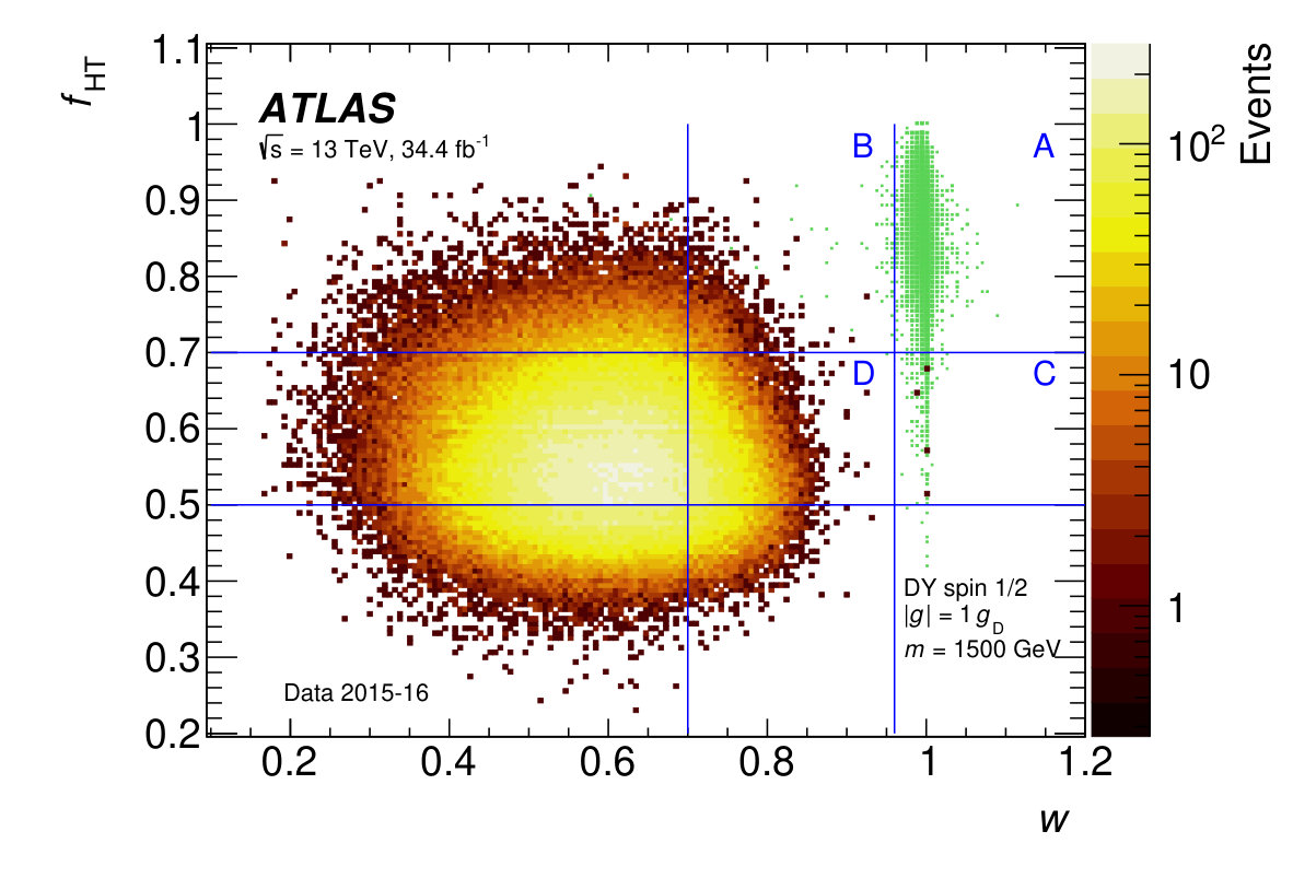 Figure 1
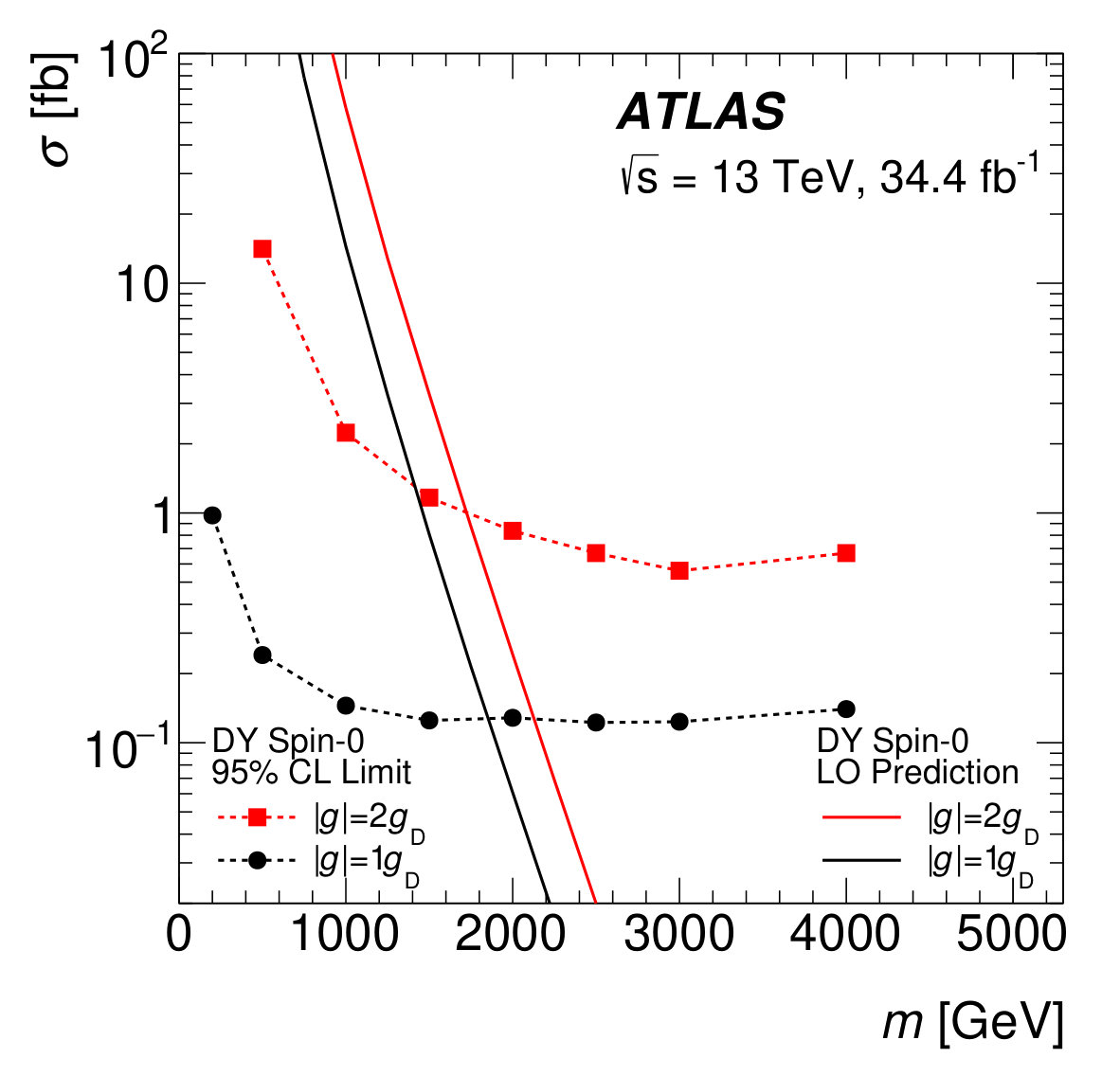 Figure 2
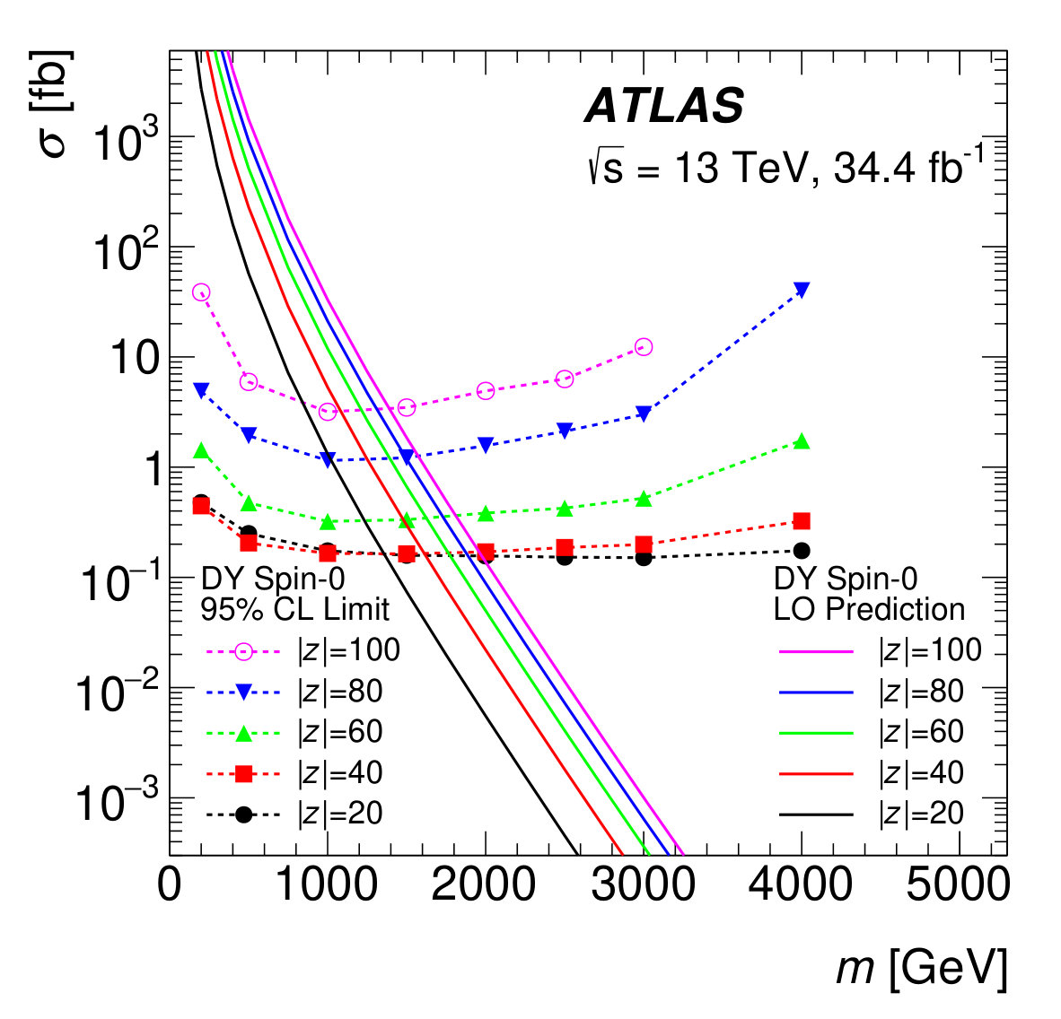 Figure 2
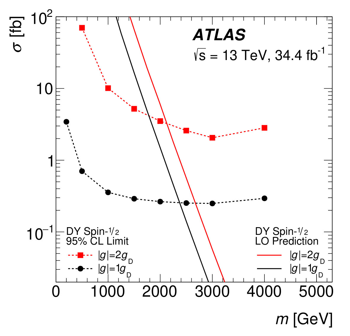 Figure 2
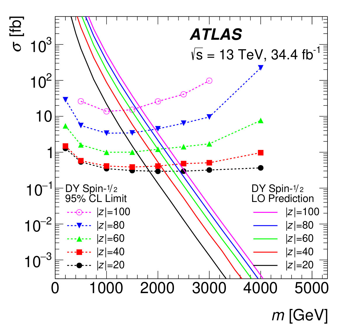 Figure 2
| Lower limits on the mass of Drell–Yan magnetic monopoles and HECOs [GeV] | |||||||
| Spin-0 | 1850 | 1725 | 1355 | 1615 | 1625 | 1495 | 1390 |
| Spin-1/2 | 2370 | 2125 | 1830 | 2050 | 2000 | 1860 | 1650 |
Peer Reviews
No public reviews on file for this paper yet. If you reviewed it on a platform where reviews are public (OpenReview, ICLR, NeurIPS, ICML), you can paste yours below so the community can read it here.
Videos
No videos yet. Explain this paper in a talk, walkthrough, or lecture? Add one.
\AtlasTitle
Search for magnetic monopoles and stable high-electric-charge objects in 13 TeV proton–proton collisions with the ATLAS detector \AtlasAbstractA search for magnetic monopoles and high-electric-charge objects is presented using 34.4 fb*-1* of 13 TeV collision data collected by the ATLAS detector at the LHC during 2015 and 2016. The considered signature is based upon high ionization in the transition radiation tracker of the inner detector associated with a pencil-shape energy deposit in the electromagnetic calorimeter. The data were collected by a dedicated trigger based on the tracker high-threshold hit capability. The results are interpreted in models of Drell–Yan pair production of stable particles with two spin hypotheses (0 and 1/2) and masses ranging from 200 GeV to 4000 GeV. The search improves by approximately a factor of five the constraints on the direct production of magnetic monopoles carrying one or two Dirac magnetic charges and stable objects with electric charge in the range and extends the charge range to . \AtlasRefCodeEXOT-2017-20 \PreprintIdNumberCERN-EP-2019-084 \arXivId1905.10130 \HepDataRecord10.17182/hepdata.89874 \AtlasJournalRefPhys. Rev. Lett. 124 (2020) 031802 \AtlasDOI10.1103/PhysRevLett.124.031802 \AtlasCoverSupportingNoteMonopole/HECO search 13 TeV 2016https://cds.cern.ch/record/2267571
The symmetry between electric and magnetic charge in Maxwell’s Equations and the explanation for electric charge quantization resulting from Dirac’s quantum description of the magnetic monopole [1, 2] are compelling arguments for its existence. Neither the spin nor the mass of a Dirac monopole is theoretically constrained. While monopoles appearing in grand unification theories [3, 4] typically have masses of the order of the unification scale ( GeV), some extensions of the Standard Model predict electroweak monopoles with masses as low as 4 TeV [5, 6, 7, 8, 9]. TeV-mass monopoles can be produced in the early Universe thermally or via the Kibble mechanism [10, 11] in cosmological scenarios with a low reheat temperature after inflation [12].
Dirac’s argument predicts the fundamental magnetic charge to be , 111In this definition, is in SI units and is a dimensionless quantity. where is the Dirac charge, is the fine structure constant, is an integer number, is the unsigned electron charge and is the speed of light in vacuum. This implies that a high-velocity Dirac monopole of magnetic charge would interact with matter in a manner similar to that of an ion of electric charge , where is in units of . Since the energy loss is proportional to the square of the charge, a monopole with would deposit 4700 times more energy by ionization than a proton. The high stopping power also results in the production of a large number of -rays. These two features result in a high-ionization signature that is also expected in the case of exotic stable high-electric-charge objects (HECOs), which may include, for example, aggregates of - [13] or -quark matter [14], -balls [15, 16], and micro black-hole remnants [17].
This Letter presents a search for magnetic monopoles and HECOs, collectively referred to as highly ionizing particles, or HIPs, using 34.4 fb*-1* of 13 TeV proton–proton () collision data collected by the ATLAS detector at the CERN Large Hadron Collider (LHC) during 2015 and 2016. Events containing at least one high-ionization object are selected. The results are interpreted in models of spin-0 and spin-1/2 Drell–Yan pair production of stable particles carrying one or two Dirac magnetic charges or an electric charge in the range with masses ranging from 200 GeV to 4000 GeV.
Should monopoles exist in the mass range accessible to a particle accelerator, they could be copiously produced at the LHC. If they were detected, the measured mass and coupling would severely restrict cosmological scenarios. Since the numerous searches for monopoles of cosmological origin in cosmic rays and in matter [18, 19] have limited sensitivity to TeV-mass HIPs, the cross-section limits for low-mass HIPs from searches at colliders [20, 21, 22, 23, 24, 25, 26, 27, 28, 29, 30, 31, 32, 33, 34] are 6–9 orders of magnitude more stringent. The first LHC searches for HECOs and monopoles were made by the ATLAS Collaboration in 8 TeV collisions [24, 25] by exploiting the high-ionization signature. The higher collision energy, the five times larger dataset and improvements in the trigger extend the sensitivity of the present search. While the previous search studied , the present search considers monopoles up to , which are motivated by Schwinger, who showed that must be even for particles possessing both electric and magnetic charge [35, 36, 37]. The ATLAS monopole searches [25, 27] are complementary to those performed using the dedicated MoEDAL experiment [28, 29, 30, 31], which uses an induction technique to detect the magnetic flux of monopoles trapped in matter. While MoEDAL is sensitive to magnetic charges up to , the present ATLAS search is able to set significantly better cross-section constraints for and , the charge range in which it has a good acceptance [38].
Unlike searches using the induction technique, the present search is sensitive to high-charge HECOs in addition to monopoles. It is complementary to the low-charge HECO searches performed by ATLAS ( [26, 32, 34]) and CMS ( [33]), all of which used muon triggers. A muon trigger is not appropriate for high-charge HECOs, which typically stop in the electromagnetic calorimeter, due to the charge-square dependence of . In LHC Run 1, ATLAS probed electric charges up to [24, 27] via the high-ionization signature. The present analysis is able to probe HECOs up to , thereby reaching the previously unexplored charge range predicted for -quark matter [13].
The present search exploits the very characteristic high-ionization signature of HIPs in the ATLAS detector [39]. The ATLAS transition radiation tracker (TRT), which is the outermost tracker of the inner detector, consists of a barrel ( and radius 0.563 m m) 222ATLAS uses a right-handed coordinate system with its origin at the nominal interaction point (IP) in the center of the detector and the -axis coinciding with the axis of the beam pipe. The -axis points from the IP to the center of the LHC ring, and the -axis points upward. Cylindrical coordinates (, ) are used in the transverse plane, being the azimuthal angle around the beam pipe. The pseudorapidity is defined in terms of the polar angle as . with 4-mm-diameter straws oriented parallel to the beam-line, and two endcaps () with straws oriented radially. In LHC Run 2, 56% of the straws were filled with xenon gas while the others were filled with argon gas. Energy deposits in a TRT straw greater than 200 eV, called low-threshold (LT) hits, are used for tracking. The high-threshold (HT) hits, which result from energy deposits exceeding 6 keV in Xe (2 keV in Ar) are typically used for electron identification, but can also indicate the presence of a highly ionizing particle. A 2 T superconducting solenoid surrounds the TRT. The lead/liquid-Ar (LAr) barrel electromagnetic (EM) calorimeter lies outside the solenoid in the region. It is divided into three shower-depth layers: EM1, EM2 and EM3, with accordion-shape electrodes and lead absorbers. The EM2 layer has the largest sampling depth ( to ); its cell granularity is . In the region, an additional presampler layer is used to measure the energy lost in front of the calorimeter. As a HIP traverses the TRT, a localized region of high ionization density with many HT hits from both the HIP and the -rays is produced in its wake. HIPs slow down (and usually stop) in the EM calorimeter, where they leave a pencil-shape energy deposit since they do not induce a shower, being much heavier than the electron.
Signal efficiency estimates rely heavily on simulations, which use the Geant4 framework [40, 41] to model the HIP propagation and behavior in ATLAS. The detector simulation includes the full ATLAS geometry, descriptions of monopole acceleration in the solenoidal magnetic field, ionization energy losses in matter [42, 43, 44, 45], -electron production along the HIP trajectory, and a model accounting for electron–ion recombination in the LAr EM calorimeter [46]. For monopoles, the trajectory in the solenoidal magnetic field is straight in the – plane and bends in the – plane and the Bethe–Bloch formula is modified [42, 43] to account for the velocity-dependent Lorentz force. The interaction of HIPs with matter is independent of HIP spin.
The Drell–Yan (DY) pair-production process is used to estimate the kinematic distributions and cross sections of spin-0 and spin-1/2 HIPs in the relevant ranges of charge and mass. The MadGraph5_aMC@NLO [47] event generator was used to model leading-order HIP DY pair production from the initial state via quark–antiquark annihilation into a virtual photon. The charge-squared dependence of the HIP coupling to the photon implies divergences in the perturbative expansion beyond leading order [48]. Pythia version 8.212 [49, 50] was employed for the hadronization and the underlying-event generation, using the NNPDF2.3 [51] parton distribution functions of the proton with the A14 [52] set of tuned parameters (‘tune’). The A2 [53] tune was used for the ‘pileup’, which are additional simulated collisions overlaid on each event according to the distribution of the number of interactions per bunch crossing, , in the data. Fully simulated HIP Monte Carlo (MC) samples are computationally intensive due to the high ionization. To minimize the number of such MC samples, model-independent efficiency maps, finely binned in kinetic energy and , are produced from fully simulated single-particle samples of a given mass and charge. The spin-0 DY HIP four-vectors from the generator are used to sample the maps in order to derive the spin-0 DY HIP selection efficiencies. The DY spin-1/2 selection efficiencies are derived from fully simulated DY samples, which are also used to validate the results obtained by sampling the efficiency maps and to assign a modeling uncertainty. The selection efficiencies for spin-0 DY HIPs are higher than for spin-1/2 because they have more central and harder kinetic energy distributions.
Incomplete knowledge of the simulation parameters translates into systematic uncertainties in the signal efficiencies. These uncertainties are estimated by varying the parameters within a range corresponding to an uncertainty of one standard deviation, as described in more detail in Ref. [27]. The dominant uncertainties are those due to the descriptions of the detector material and of electron–ion recombination in the EM calorimeter, each with an average relative uncertainty of 7%. Other relevant parameters include the dependence of the multiplicity of TRT LT hits on pileup , the HIP energy-loss calculation as well as the yield and range of -electrons, and the fraction of energy cross-talk between adjacent EM calorimeter cells. Additional uncertainties unrelated to detector effects include the uncertainty from MC statistics and the systematic uncertainty due to imprecise modeling or deriving DY efficiencies from the single-particle maps.
ATLAS uses a two-level trigger system [54]. Level 1 is a hardware-based trigger that defines calorimeter ‘regions of interest’ (RoI). A dedicated software-based high-level trigger (HLT), which imposes requirements on the number and fraction of TRT HT hits in a narrow region around the RoI, started collecting data in October 2015. The level-1 seed requires transverse energy GeV in the electromagnetic calorimeter. RoI candidates with GeV in conjunction with an -dependent minimum of 1 to 2 GeV of energy in the hadronic calorimeter are vetoed. This unavoidable hadronic veto requirement, which improves rejection of hadrons in analyses using electrons and photons, limits the sensitivity to low-charge HIPs, which often penetrate to the hadronic calorimeter. In contrast to the 8 TeV search [27], this veto on an energy deposit in the hadronic calorimeter is not applied to RoI candidates with GeV, thereby increasing the acceptance for the HIPs that do not stop in the EM calorimeter. Following the level-1 trigger, the HLT is used to select HIP candidates with HT hits in the TRT. The counting is done in an – wedge of size 10 mrad, where two trigger variables, and , are used to define the number and fraction of TRT HT hits, respectively. The HLT selection criteria are defined as and to control the rate while maintaining high signal efficiency for high-charge HIPs. In addition, a pseudorapidity requirement of is applied to avoid the forward regions, which contain more backgrounds due to multijet events producing a higher rate of level-1 trigger seeds.
In this search, the HIP signal sensitivity is governed by the DY kinematic distributions and the dependence of the stopping power on two variables: the square of the charge and the velocity relative to the speed-of-light . For HECOs, is proportional to whereas it varies as for monopoles [42, 43]. The main source of signal loss is due to HIPs failing to produce a level-1 trigger RoI, because they either stop before the EM calorimeter (e.g., high-charge HIPs), deposit too little energy in the calorimeter or penetrate to the hadronic calorimeter and invoke the veto (e.g., low-charge HIPs). The probability for a HIP from DY pair production to induce a level-1 trigger signal is around 60% for HECOs with and 55% for monopoles with and decreases to 18% for and 10% for . For HIPs with that pass the level-1 trigger, the efficiency to satisfy the HLT and the remaining offline selection, described below, is generally 25% to 60%.
Any data that fail the electron–photon data quality requirements are discarded as are events flagged as containing noise in the LAr calorimeter. The event selection then starts by identifying events containing at least one candidate featuring a topological cluster of EM calorimeter cells [55] with GeV in the region. The remaining selection is based on two powerful background-discriminating variables, denoted and . The selected EM cluster candidates are used to seed the variable, which is similar to the trigger variable except that an 8-mm-wide rectangular road is used instead of a 10-mrad wedge, to better confine the hit counting to the region closest to the HIP trajectory. The variable gives a measure of the lateral energy dispersion of the EM cluster candidate. For each EM cluster candidate, the associated energy contained in the presampler, EM1 layer and EM2 layer is denoted by , and , respectively. Three variables (, 1, 2) are defined as the fraction of EM cluster energy contained in the two most energetic cells in the presampler, the four most energetic cells in EM1, and the five most energetic cells in EM2, respectively. If the cluster energy in layer is confined to a single cell, then , consistent with the narrow shower expected for HIPs. In each layer, the number of cells is chosen to optimize the signal efficiency and the discrimination power between HIPs and electron or jet backgrounds. The combined lateral energy dispersion is thus defined as the average of all (, 1, 2) for which exceeds 10 GeV (relaxed to 5 GeV for ). The latter requirement ensures that only layers with energy deposits significantly above the cluster-level noise, which depends on both the cell-level noise and the cell granularity, contribute to the computation. In addition, at least one of the and requirements must be satisfied. The final selection requirements are and , a choice which maximizes the signal-to-background ratio for the majority of the signal samples.
Backgrounds are random combinations of rare processes and need to be estimated directly from the collected data. Examples of background processes that could yield high values include overlapping charged particles and noise in TRT straws. Processes that could yield high values include high-energy electrons and noise in EM calorimeter cells. The background estimation method relies on the fact that, in the background near the signal region, and are largely uncorrelated. Control regions B, C and D are defined as sidebands in and near the signal region A, as shown in Figure 1. Region A contains 90% or more of the signal for masses below 4000 GeV for all simulated charges except , where the fraction is 70%. The numbers of events observed in the control regions are , and , and the expected background is calculated as . The latter uncertainty accounts for the fact that and each depend on but in different ways, resulting in a Pearson correlation coefficient of 10%. This uncertainty was obtained by binning the – plane into -unit regions in and determining the maximum variation of the ratio of the numbers of events in the B and D regions. Simultaneous fits taking possible signal yields into account confirm that signal leakage into the B and C control regions cannot significantly affect the background estimate. As an additional cross-check, the B, C and D regions are divided into various subregions, within which the background estimation is again performed. The estimated and observed event yields are consistent in all cases.
No event was observed in the signal region A in 34.4 fb*-1* of 13 TeV collision data, consistent with the background expectation. Thus, 95% confidence-level (CL) upper limits can be set on production cross sections for various signal hypotheses, using estimates of efficiencies and their corresponding uncertainties for each HIP charge, mass and spin, as well as the uncertainty in the integrated luminosity (2.2%, estimated following the methods discussed in Ref. [56]). A [57] frequentist framework implemented in RooStats [58] is used for hypothesis testing and to calculate confidence intervals. The resulting limits are shown as a function of HIP mass in Figure 2 for monopoles and HECOs in the charge ranges where the search is sensitive for DY production with different spins. The mass dependence of the cross-section limits arises from a variation of the efficiencies with the HIP kinetic energy. The cross-section limits are relatively insensitive to the systematic uncertainties, which introduce variations no larger than 12% across all mass–charge–spin points. Model cross-section predictions are shown in Figure 2 as solid lines. The corresponding mass limits are shown in Table 1. Given the uncertainty in the predicted cross sections, these mass limits primarily serve as benchmarks for comparison with other experiments. The MoEDAL experiment [31] is able to set slightly stronger monopole mass limits because they consider photon-fusion pair production in addition to the Drell–Yan mechanism. For most masses, the present cross-section limits obtained for magnetic charge surpass by one to two orders of magnitude the best previous constraints, also set by MoEDAL [31]. The cross-section limits obtained for HECOs and for monopoles with surpass by approximately a factor of five the best constraints, set by the previous ATLAS analysis [27], and access the range for the first time.
We thank CERN for the very successful operation of the LHC, as well as the support staff from our institutions without whom ATLAS could not be operated efficiently.
We acknowledge the support of ANPCyT, Argentina; YerPhI, Armenia; ARC, Australia; FWF, BMWFW, Austria; ANAS, Azerbaijan; SSTC, Belarus; CNPq, FAPESP, Brazil; NSERC, CFI, NRC, Canada; CERN, CERN; CONICYT, Chile; CAS, NSFC, MOST, China; COLCIENCIAS, Colombia; VSC CR, MSMT CR, MPO CR, Czech Republic; DNSRC, DNRF, Denmark; IN2P3-CNRS, CEA-DRF/IRFU, France; SRNSFG, Georgia; MPG, HGF, BMBF, Germany; GSRT, Greece; RGC, Hong Kong SAR, Hong Kong China; Benoziyo Center, ISF, Israel; INFN, Italy; JSPS, MEXT, Japan; JINR, JINR; CNRST, Morocco; NWO, Netherlands; RCN, Norway; MNiSW, NCN, Poland; FCT, Portugal; MNE/IFA, Romania; NRC KI, MES of Russia, Russia Federation; MESTD, Serbia; MSSR, Slovakia; ARRS, MIZŠ, Slovenia; DST/NRF, South Africa; MINECO, Spain; SRC, Wallenberg Foundation, Sweden; Cantons of Bern and Geneva , SNSF, SERI, Switzerland; MOST, Taiwan; TAEK, Turkey; STFC, United Kingdom; DOE, NSF, United states of America. In addition, individual groups and members have received support from CRC, Compute Canada, Canarie, BCKDF, Canada; Marie Skłodowska-Curie, COST, ERDF, ERC, Horizon 2020, European Union; ANR, Investissements d’Avenir Labex and Idex, France; AvH, DFG, Germany; Herakleitos, Thales and Aristeia programmes co-financed by EU-ESF and the Greek NSRF, Greece; BSF-NSF, GIF, Israel; PROMETEO Programme Generalitat Valenciana, CERCA Generalitat de Catalunya, Spain; Leverhulme Trust, The Royal Society, United Kingdom.
The crucial computing support from all WLCG partners is acknowledged gratefully, in particular from CERN, the ATLAS Tier-1 facilities at TRIUMF (Canada), NDGF (Denmark, Norway, Sweden), CC-IN2P3 (France), KIT/GridKA (Germany), INFN-CNAF (Italy), NL-T1 (Netherlands), PIC (Spain), ASGC (Taiwan), RAL (UK) and BNL (USA), the Tier-2 facilities worldwide and large non-WLCG resource providers. Major contributors of computing resources are listed in Ref. [59].
The reference list from the paper itself. Each links out to its DOI / PubMed record.
- 1[1] P… Dirac “Quantised Singularities in the Electromagnetic Field” In Proc. Roy. Soc. A 133 , 1931, pp. 60 DOI: 10.1098/rspa.1931.0130 · doi ↗
- 2[2] P… Dirac “The Theory of Magnetic Poles” In Phys. Rev. 74 , 1948, pp. 817 DOI: 10.1103/Phys Rev.74.817 · doi ↗
- 3[3] G. ’t Hooft “Magnetic Monopoles in Unified Gauge Theories” In Nucl. Phys. B 79 , 1974, pp. 276 DOI: 10.1016/0550-3213(74)90486-6 · doi ↗
- 4[4] A.. Polyakov “Particle Spectrum in the Quantum Field Theory” In JETP Lett. 20 , 1974, pp. 194
- 5[5] Y.. Cho and D. Maison “Monopole configuration in Weinberg-Salam Model” In Phys. Lett. B 391 , 1997, pp. 360 DOI: 10.1016/S 0370-2693(96)01492-X · doi ↗
- 6[6] K. Kimm, J.. Yoon and Y.. Cho “Finite energy electroweak dyon” In Eur. Phys. J. C 75 , 2015, pp. 67 DOI: 10.1140/epjc/s 10052-015-3290-3 · doi ↗
- 7[7] J. Ellis, N.. Mavromatos and T. You “The Price of an Electroweak Monopole” In Phys. Lett. B 756 , 2016, pp. 29 DOI: 10.1016/j.physletb.2016.02.048 · doi ↗
- 8[8] S. Arunasalam and A. Kobakhidze “Electroweak monopoles and the electroweak phase transition” In Eur. Phys. J. C 77 , 2017, pp. 444 DOI: 10.1140/epjc/s 10052-017-4999-y · doi ↗