Visual Model-predictive Localization for Computationally Efficient Autonomous Racing of a 72-gram Drone
Shuo Li, Erik van der Horst, Philipp Duernay, Christophe De Wagter and, Guido C.H.E. de Croon

TL;DR
This paper introduces a lightweight, efficient vision-based localization method for autonomous drone racing, demonstrated on the world's smallest racing drone, achieving high speeds with minimal computational resources.
Contribution
The authors develop a novel, computationally efficient localization algorithm that fuses race gate detections with model predictions, enabling fast autonomous racing on ultra-light drones.
Findings
Achieved an average speed of 2m/s in flight tests
Demonstrated the smallest autonomous racing drone at 72g
Outperformed traditional Kalman filtering in low-frequency visual updates
Abstract
Drone racing is becoming a popular e-sport all over the world, and beating the best human drone race pilots has quickly become a new major challenge for artificial intelligence and robotics. In this paper, we propose a strategy for autonomous drone racing which is computationally more efficient than navigation methods like visual inertial odometry and simultaneous localization and mapping. This fast light-weight vision-based navigation algorithm estimates the position of the drone by fusing race gate detections with model dynamics predictions. Theoretical analysis and simulation results show the clear advantage compared to Kalman filtering when dealing with the relatively low frequency visual updates and occasional large outliers that occur in fast drone racing. Flight tests are performed on a tiny racing quadrotor named "Trashcan", which was equipped with a Jevois smart-camera for a…
Click any figure to enlarge with its caption.
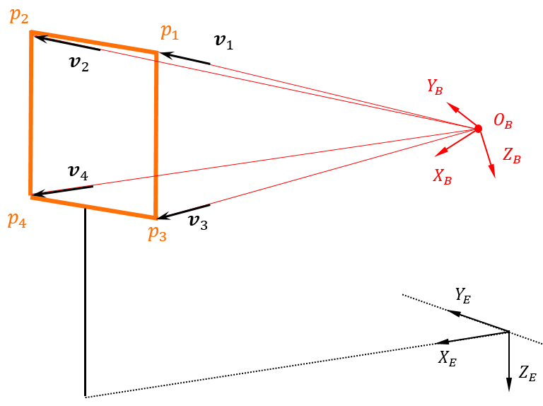 Figure 1
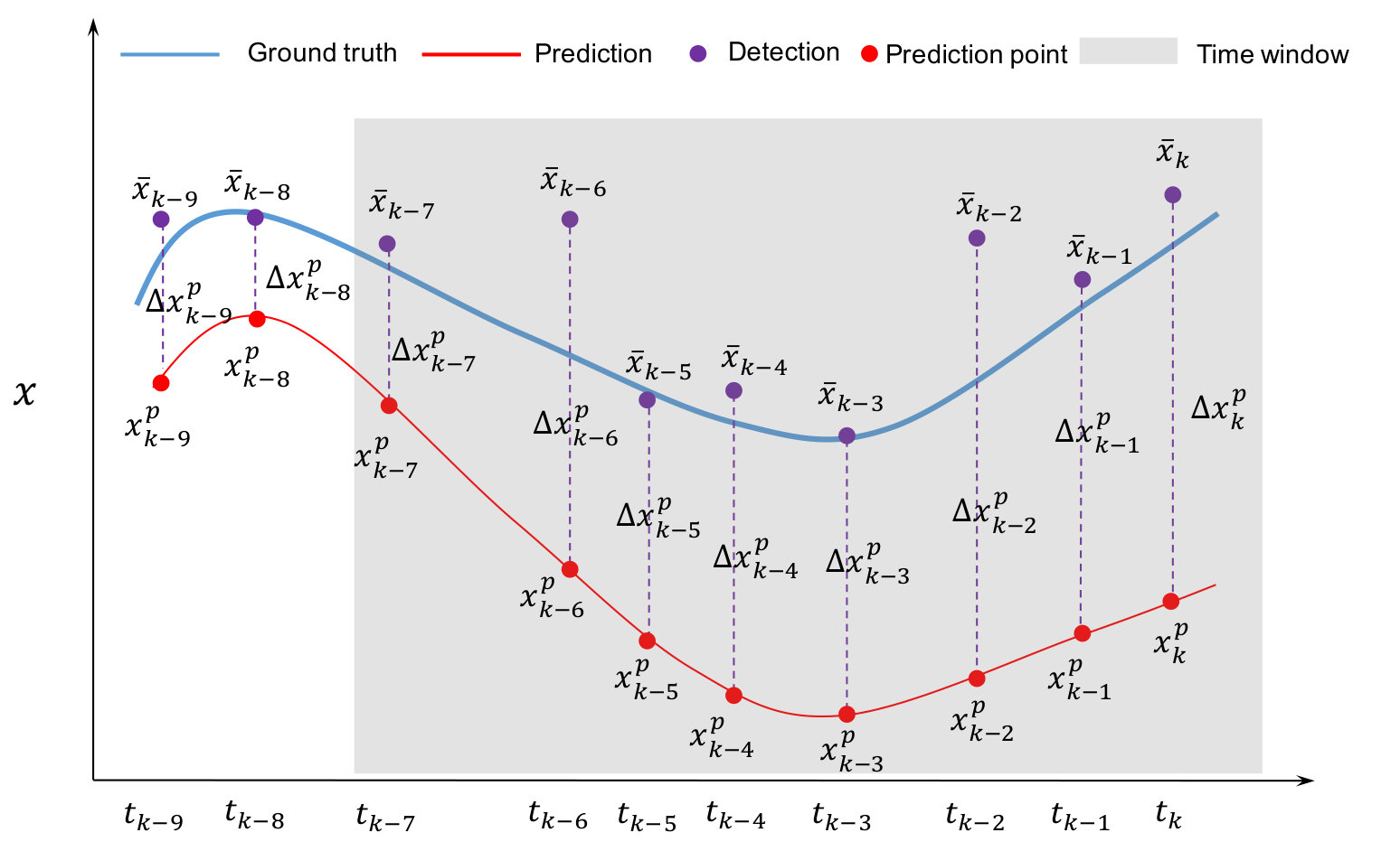 Figure 2
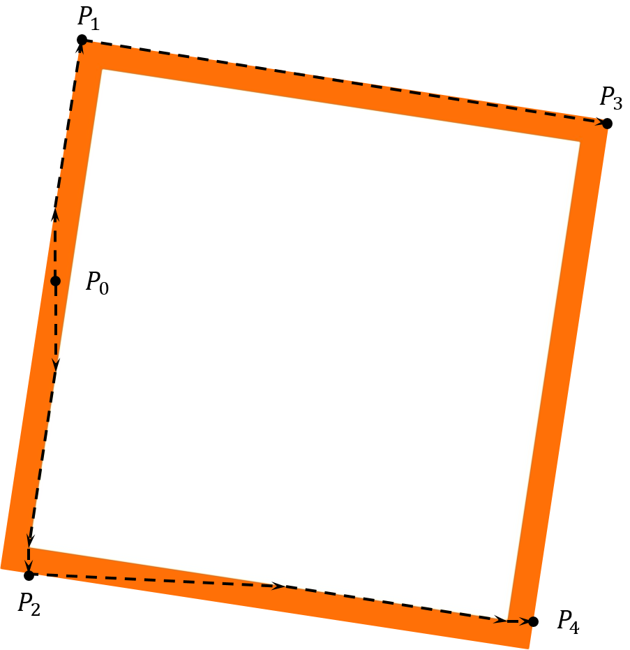 Figure 3
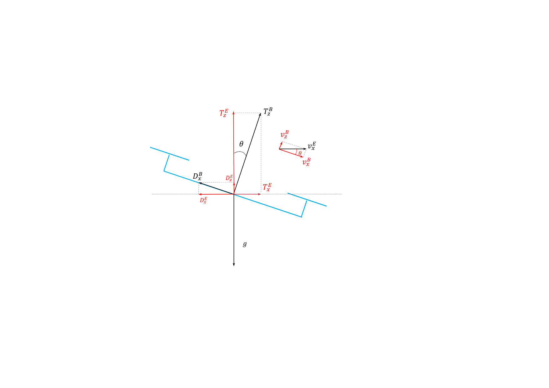 Figure 4
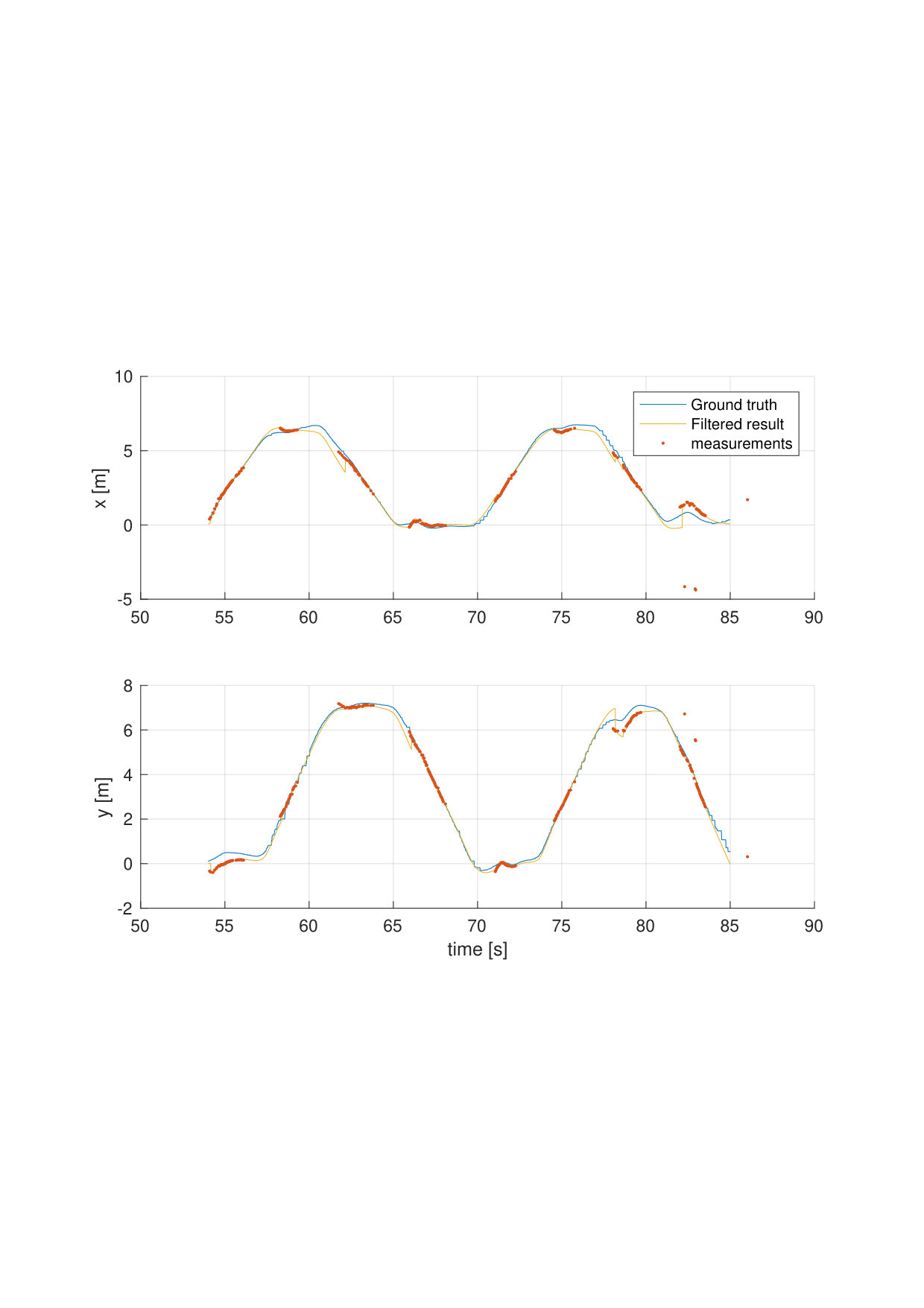 Figure 5
 Figure 6
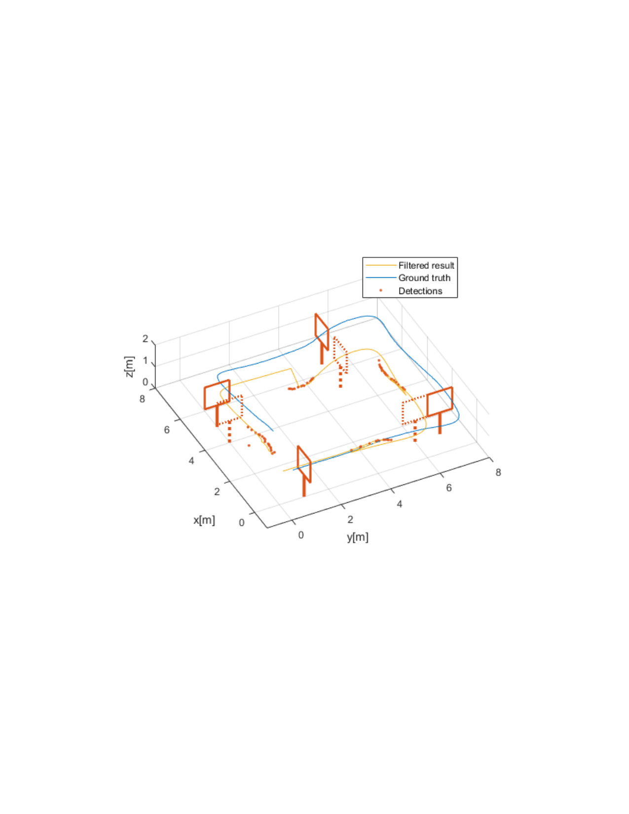 Figure 7
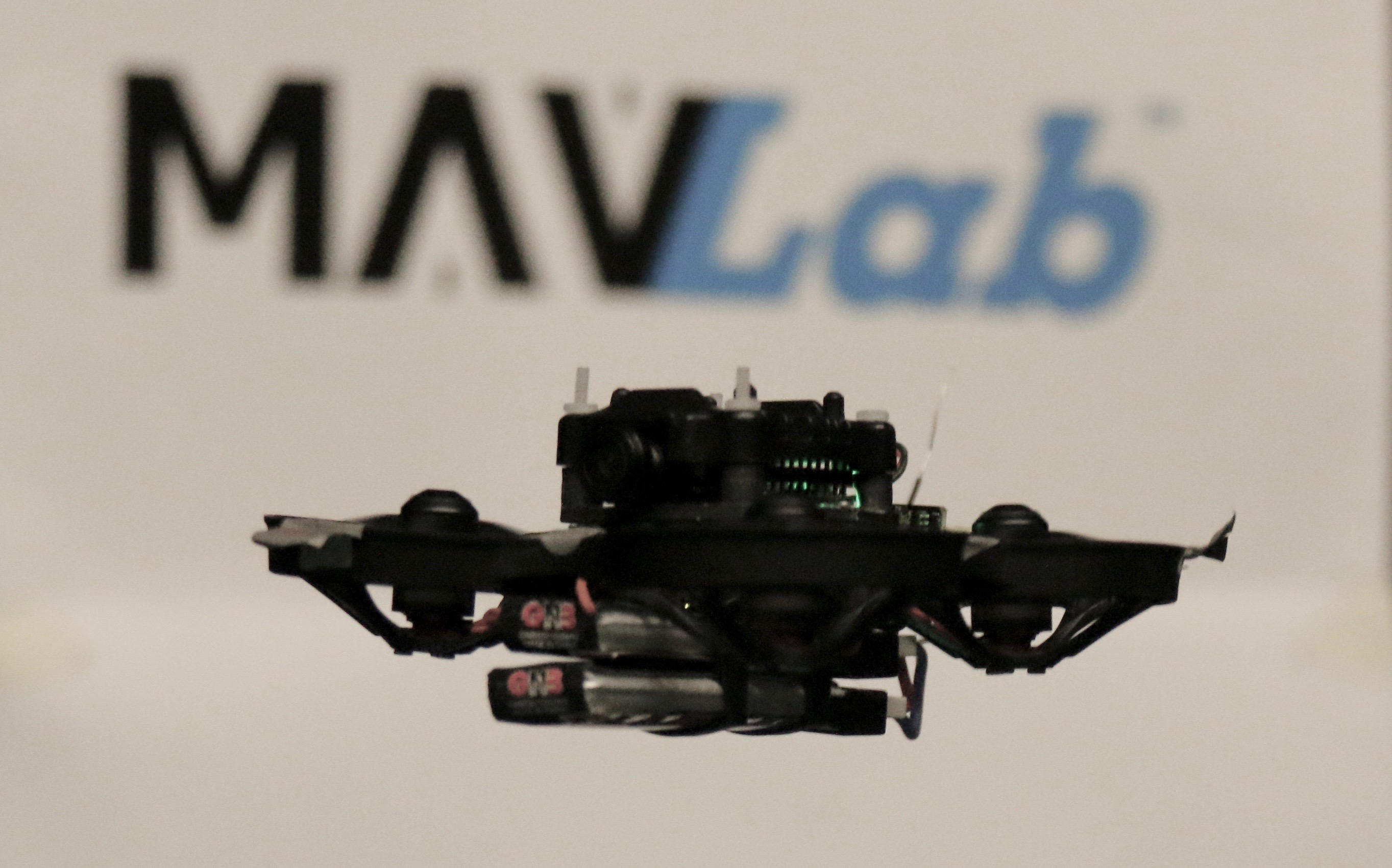 Figure 8
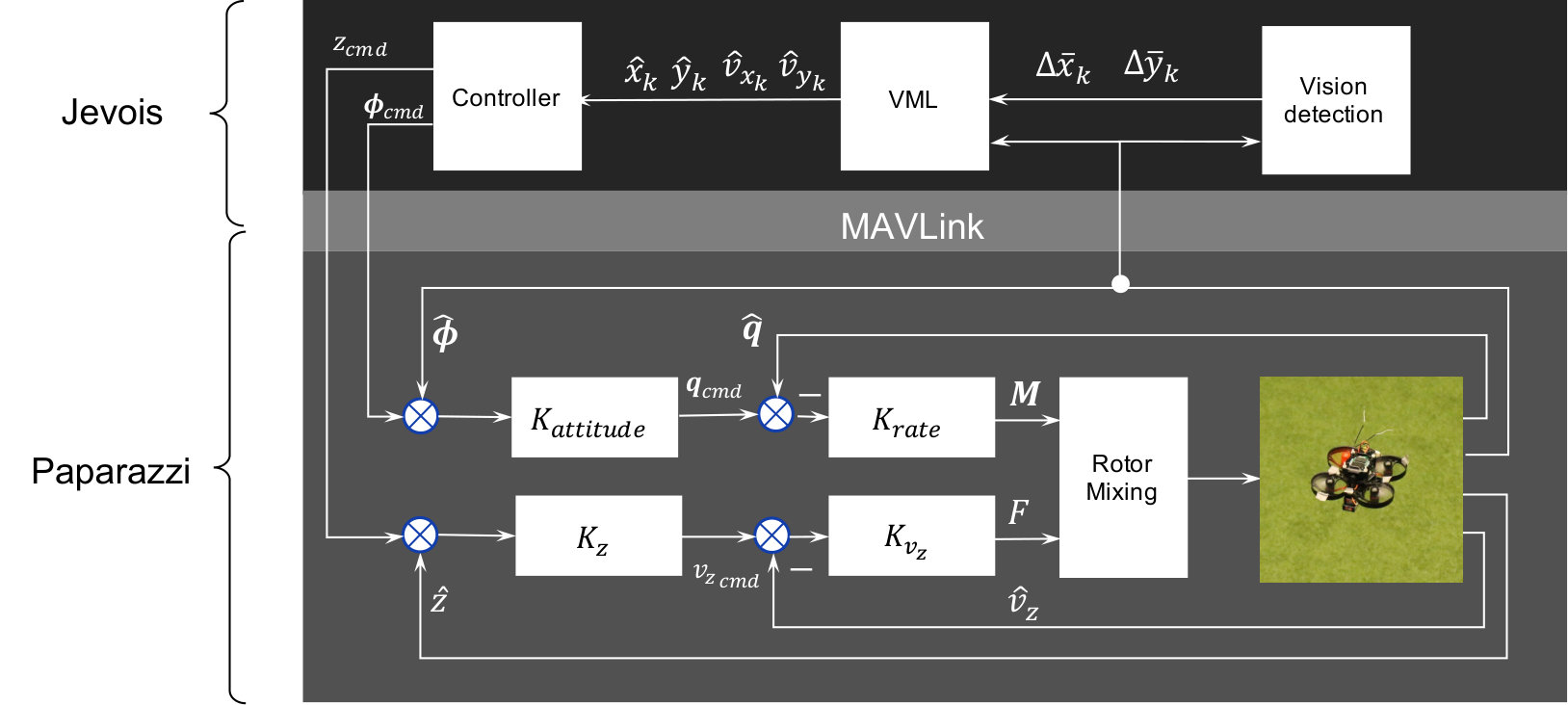 Figure 9
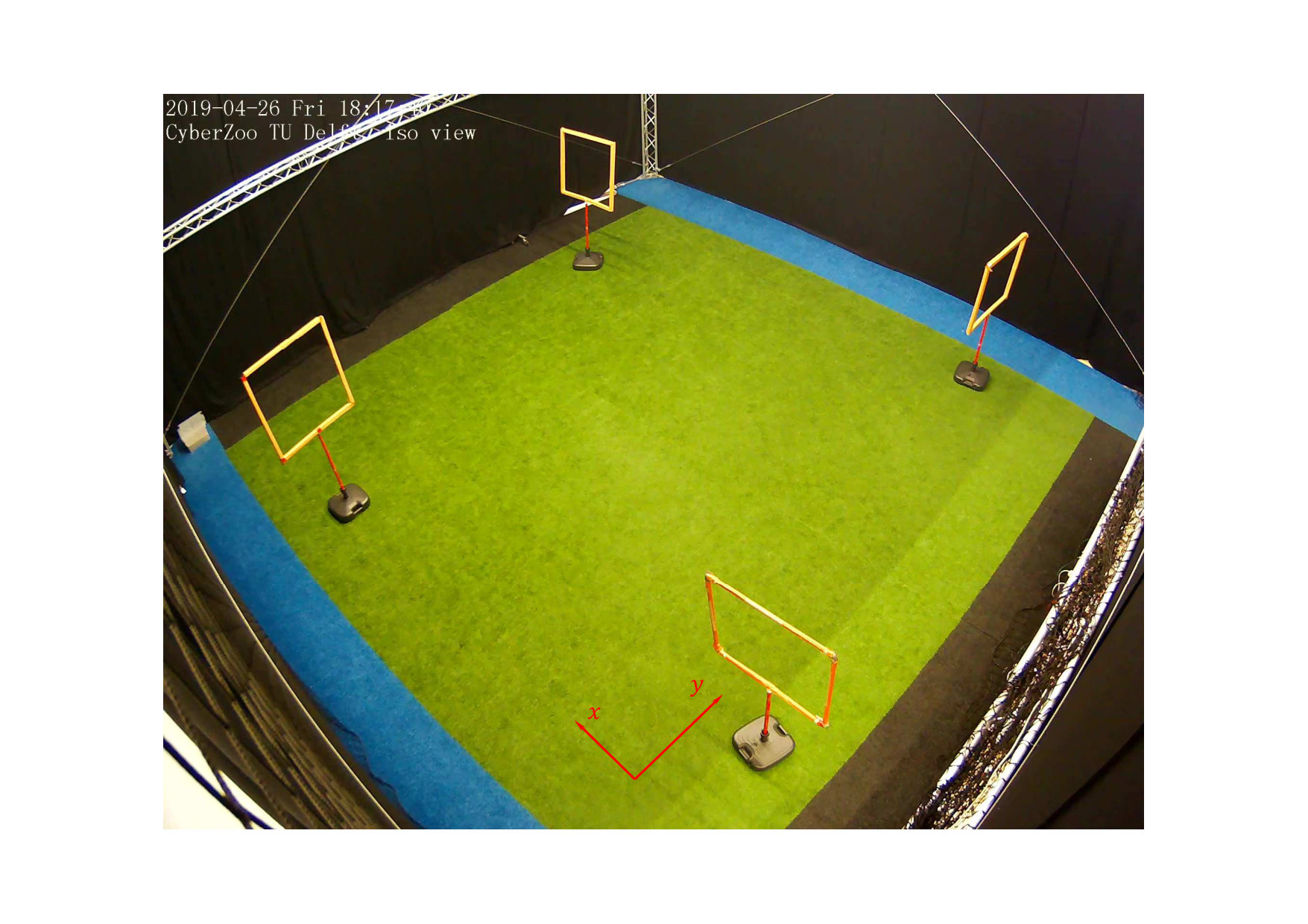 Figure 10
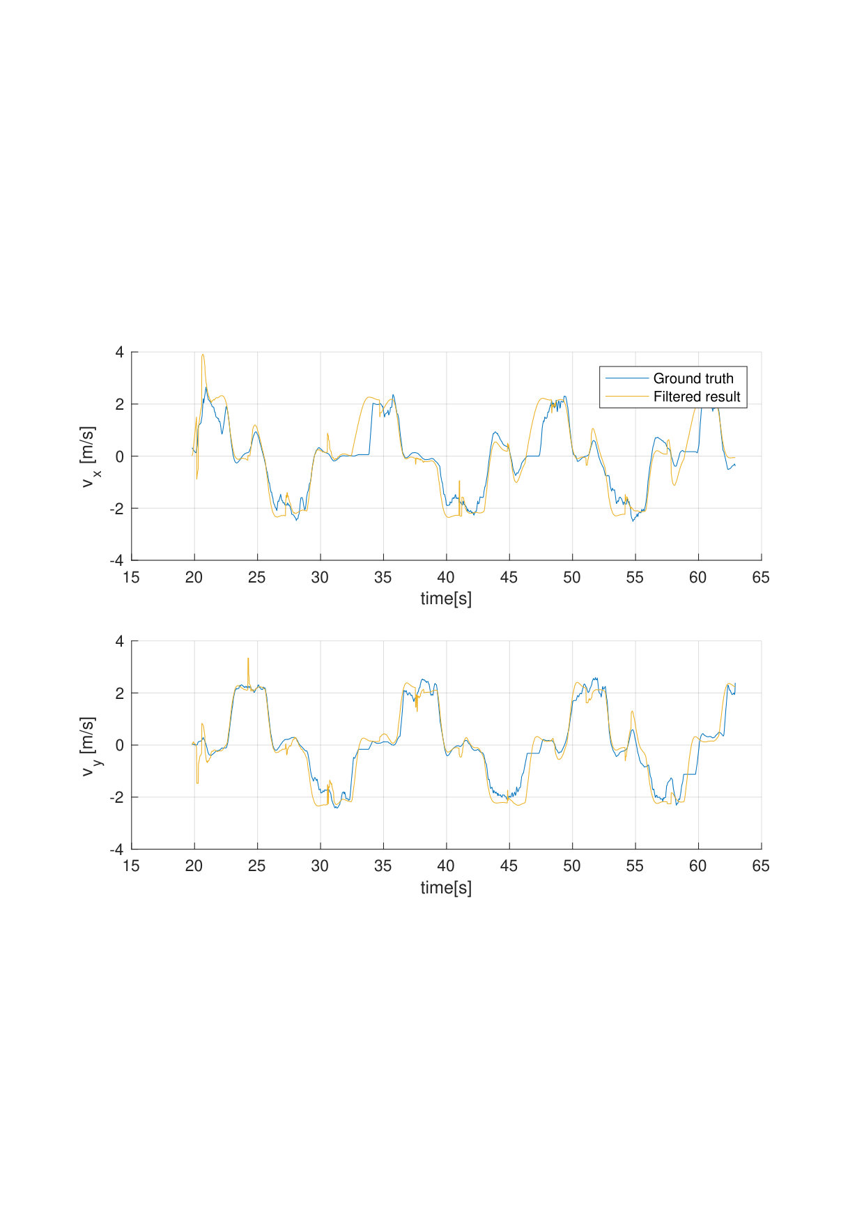 Figure 11
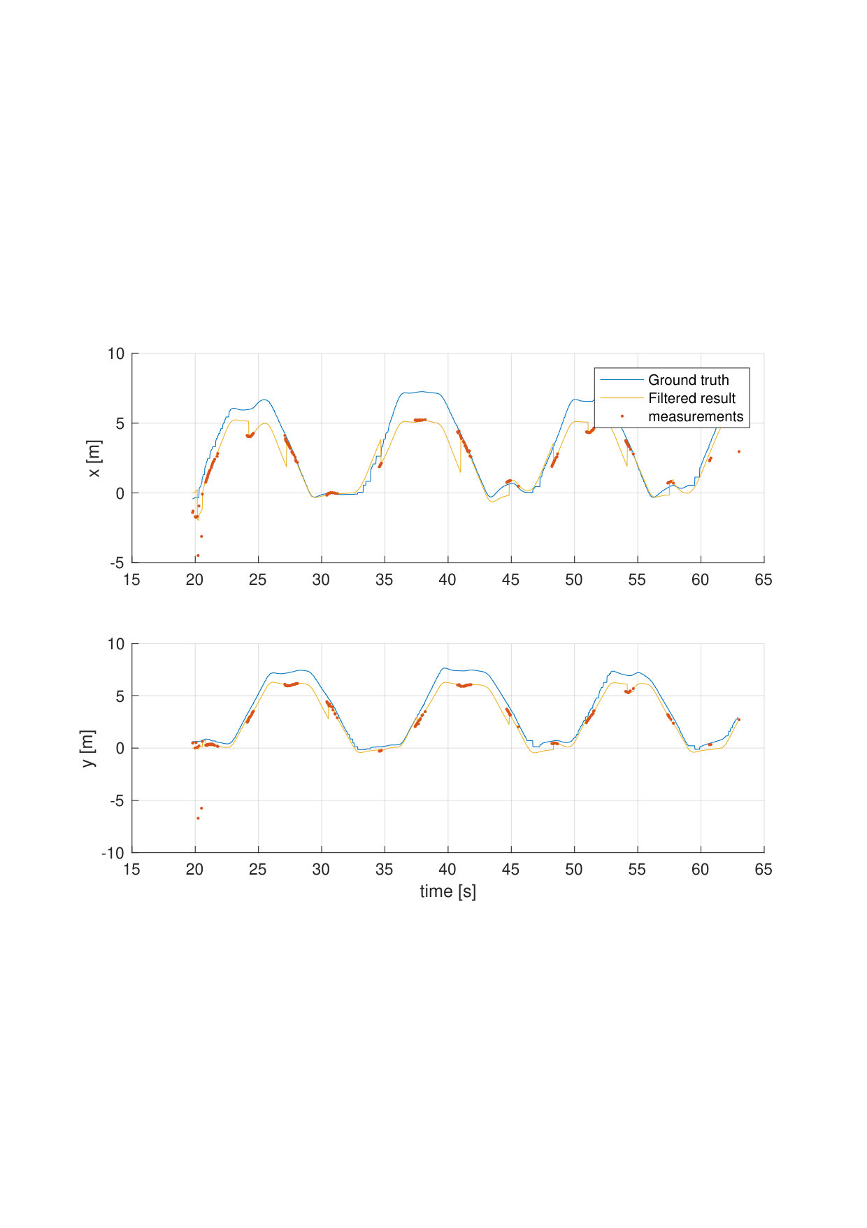 Figure 12
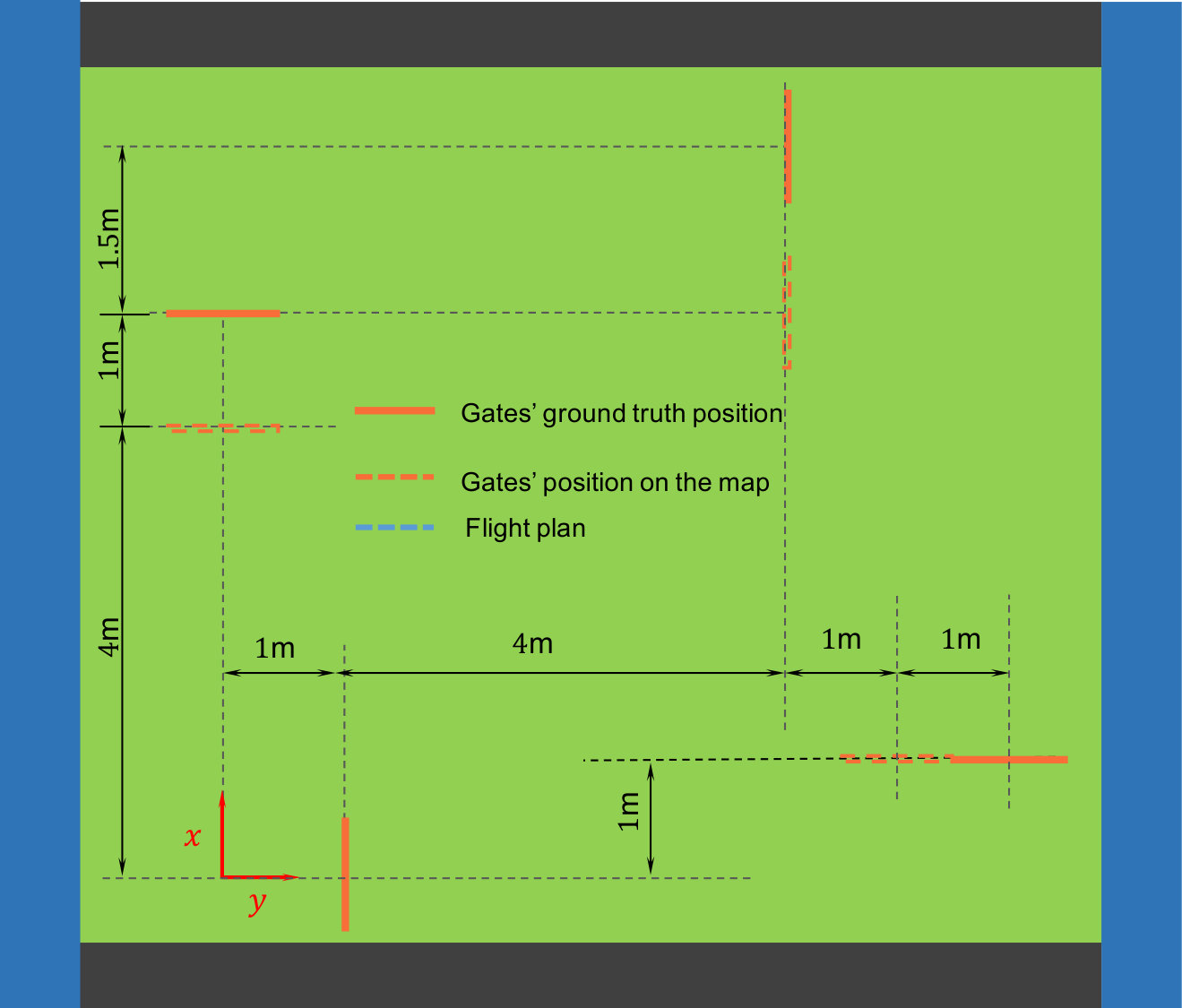 Figure 13
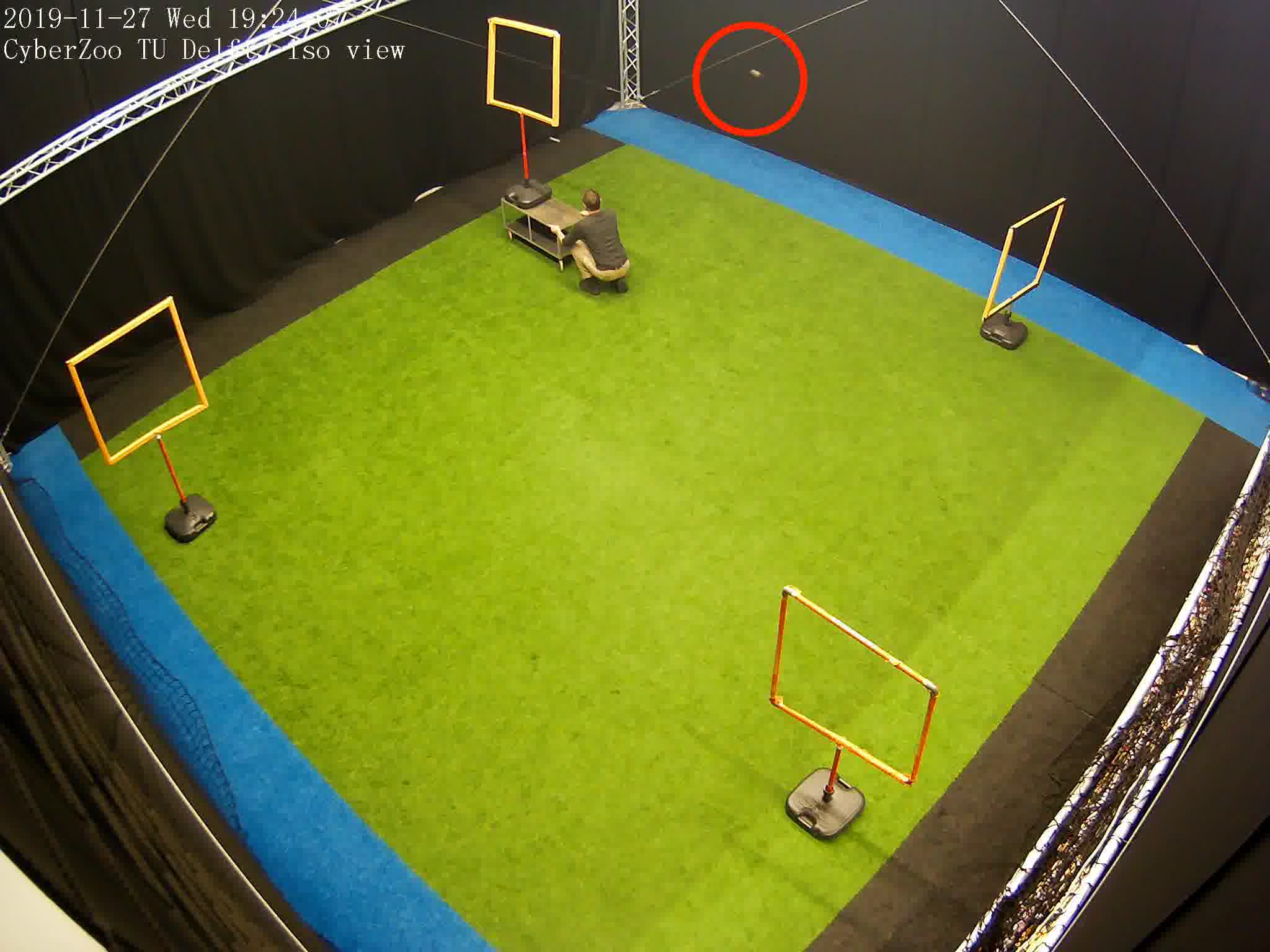 Figure 14
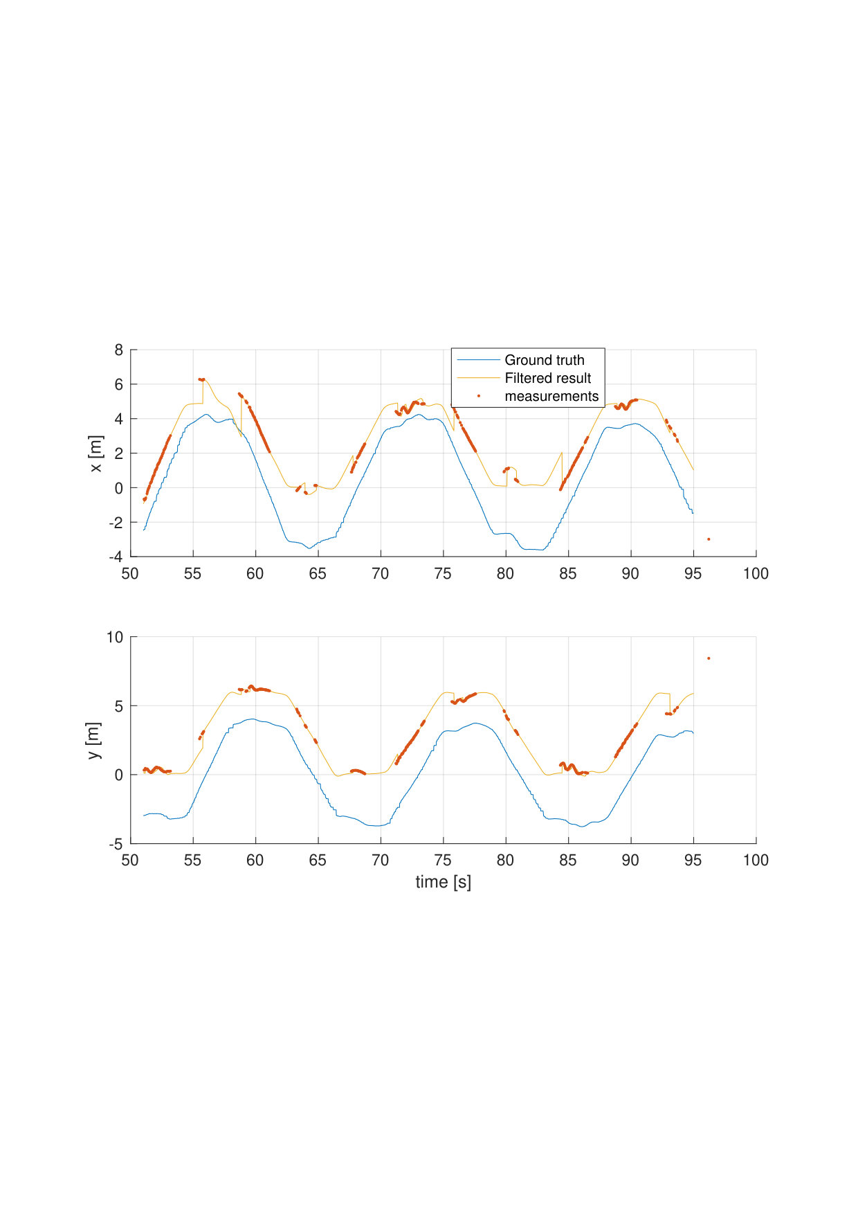 Figure 15
 Figure 16
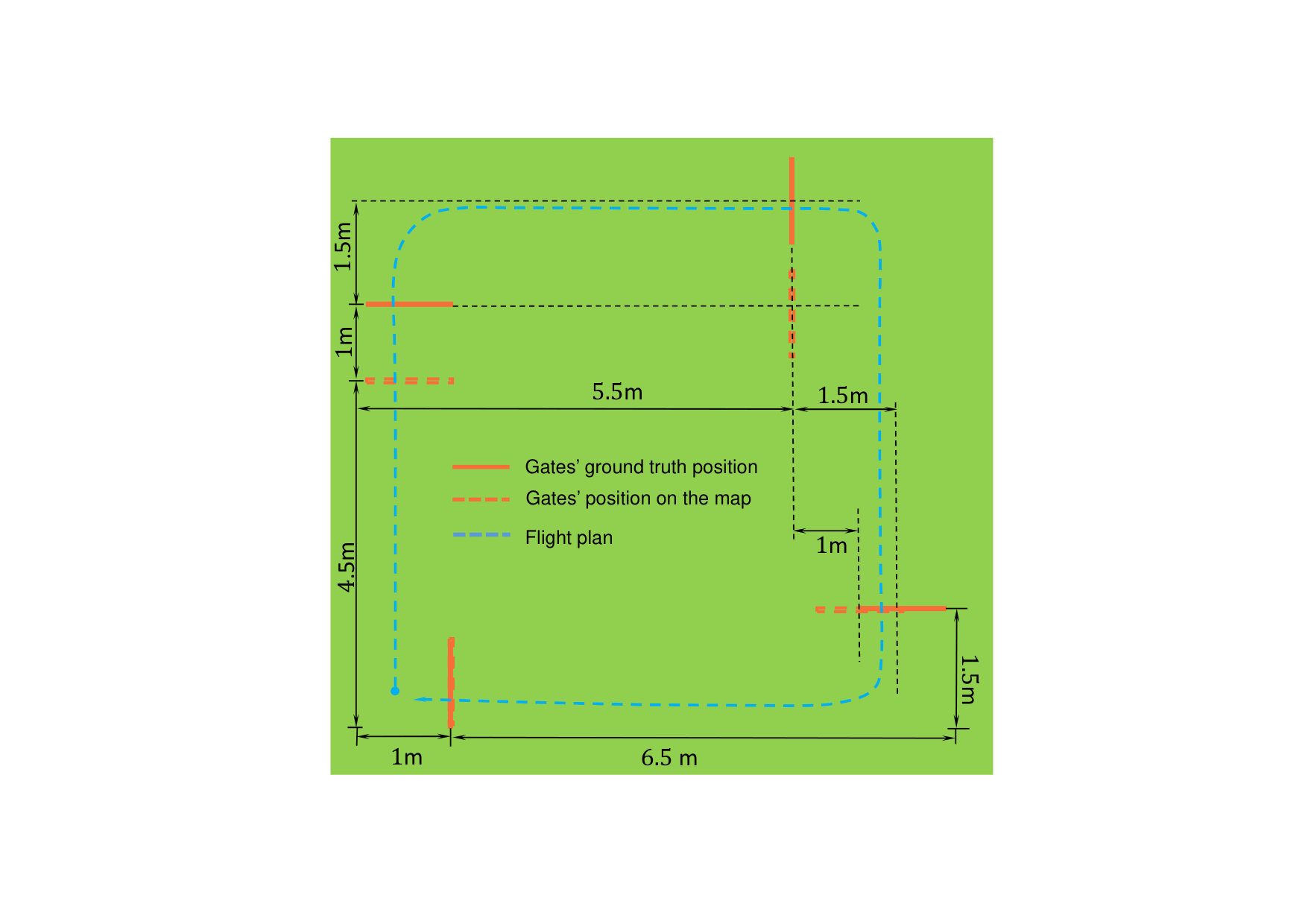 Figure 17
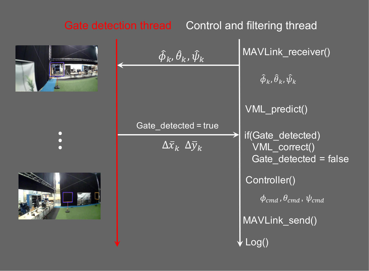 Figure 18
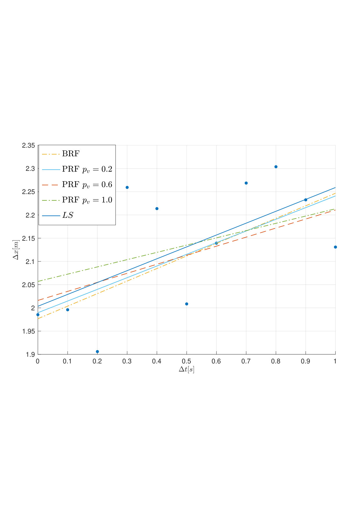 Figure 19
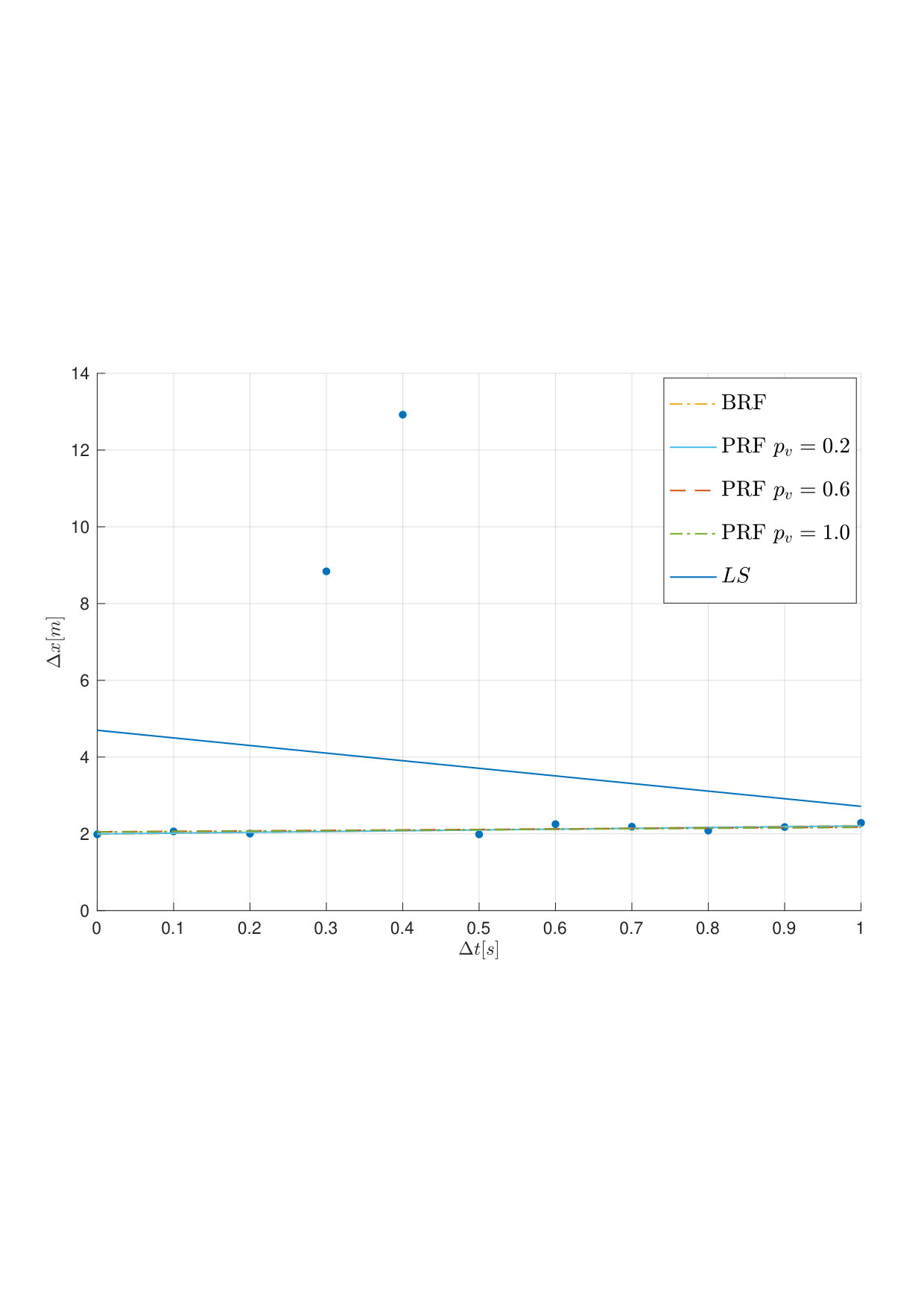 Figure 20
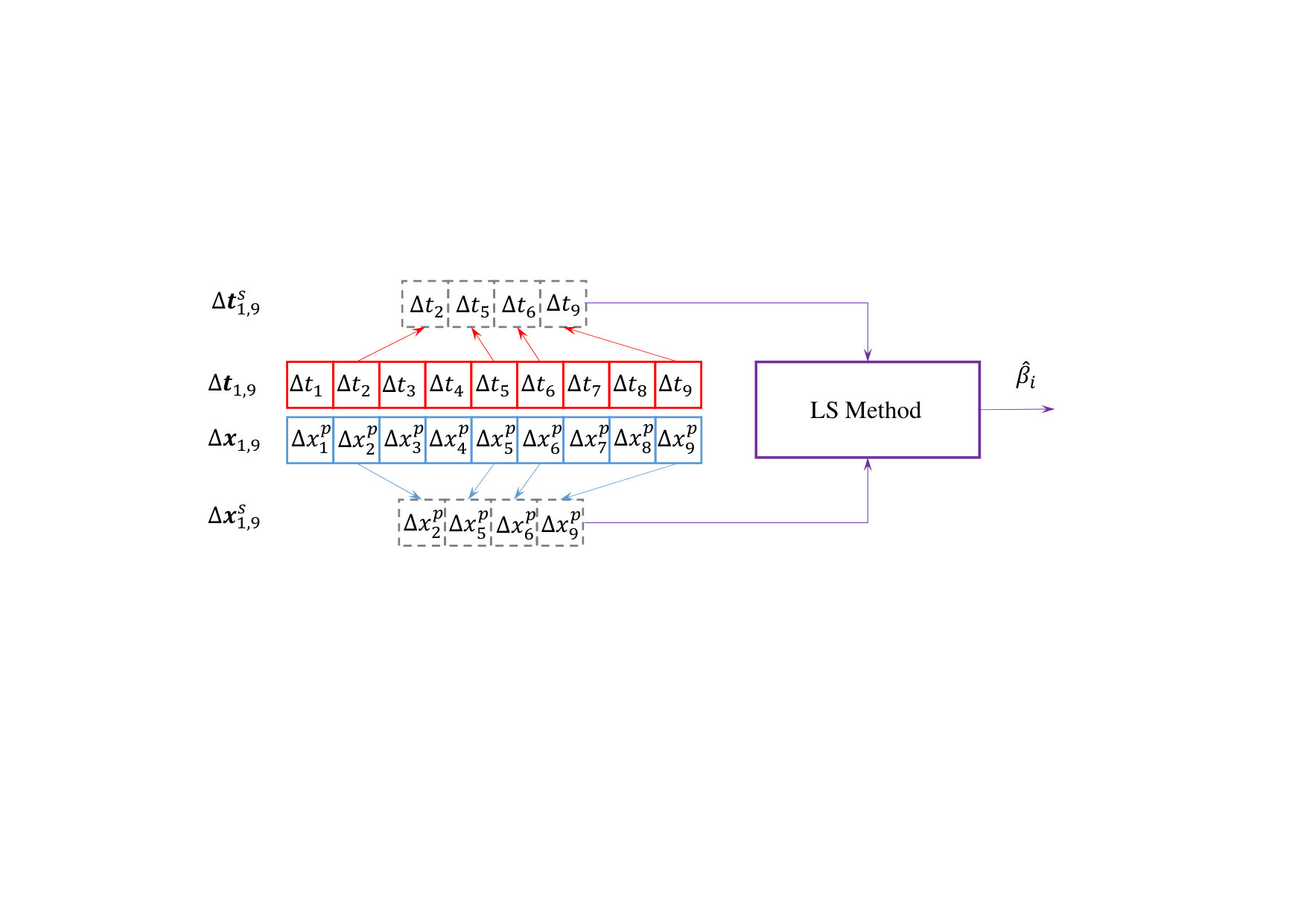 Figure 21
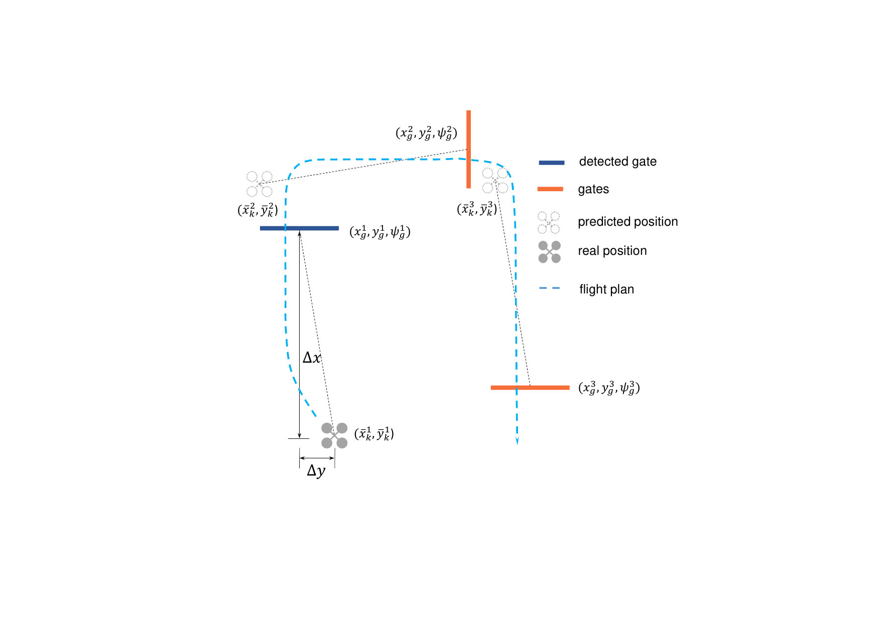 Figure 22
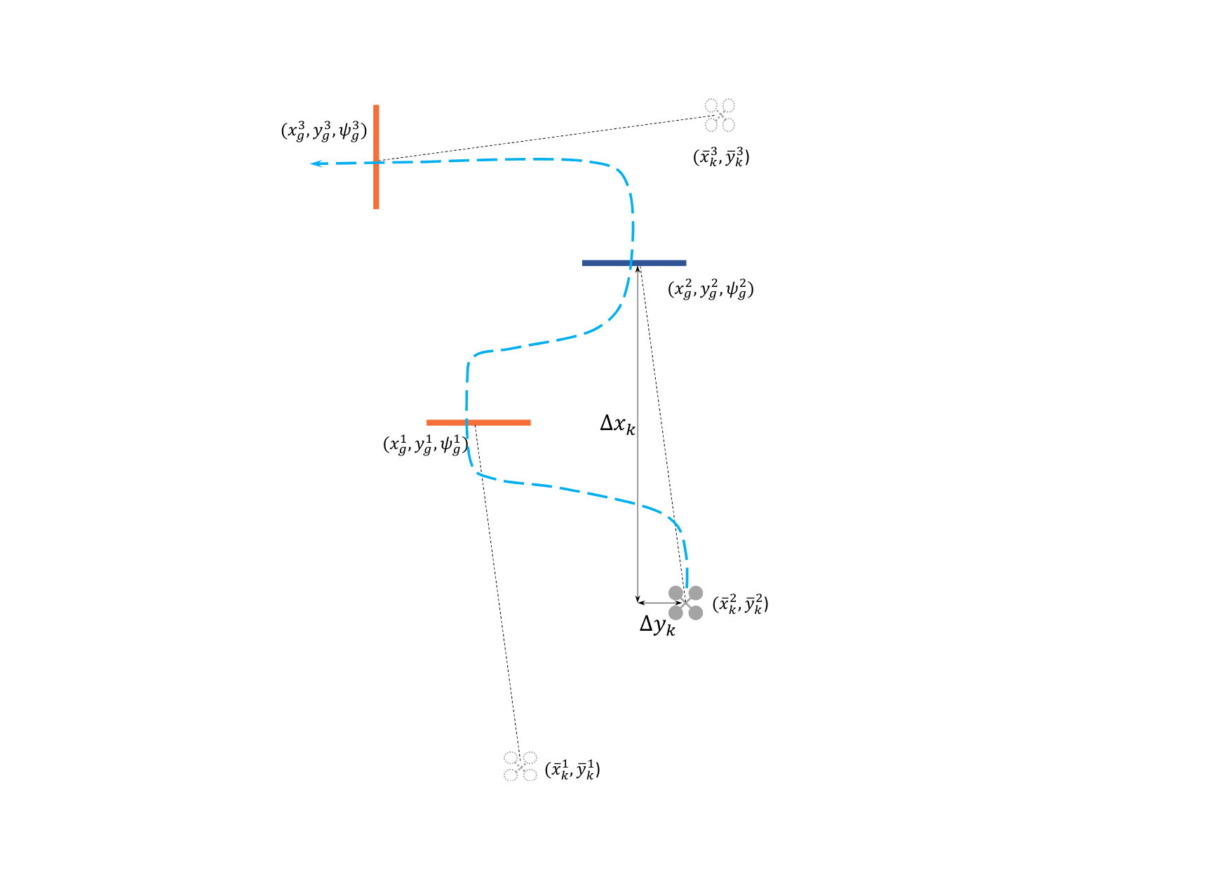 Figure 23
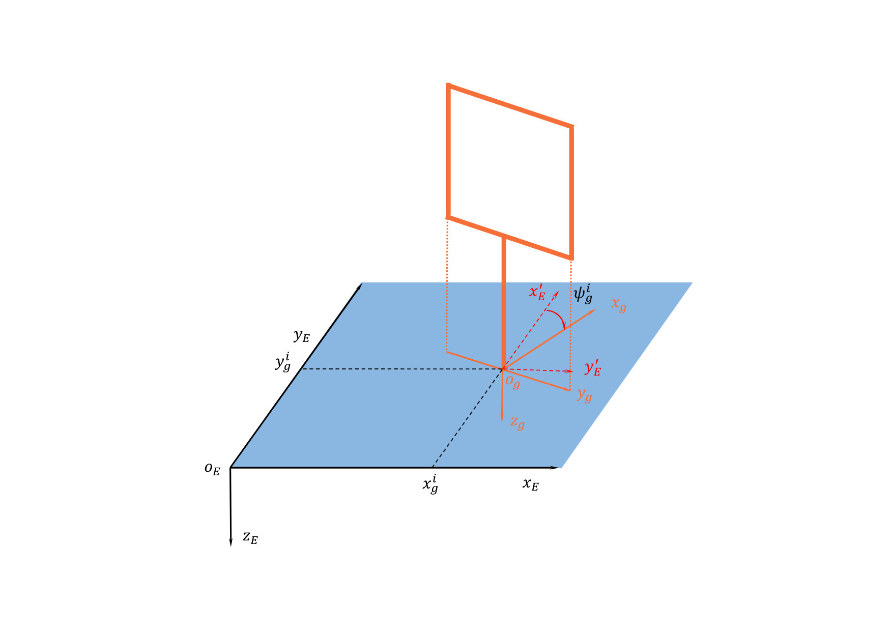 Figure 24
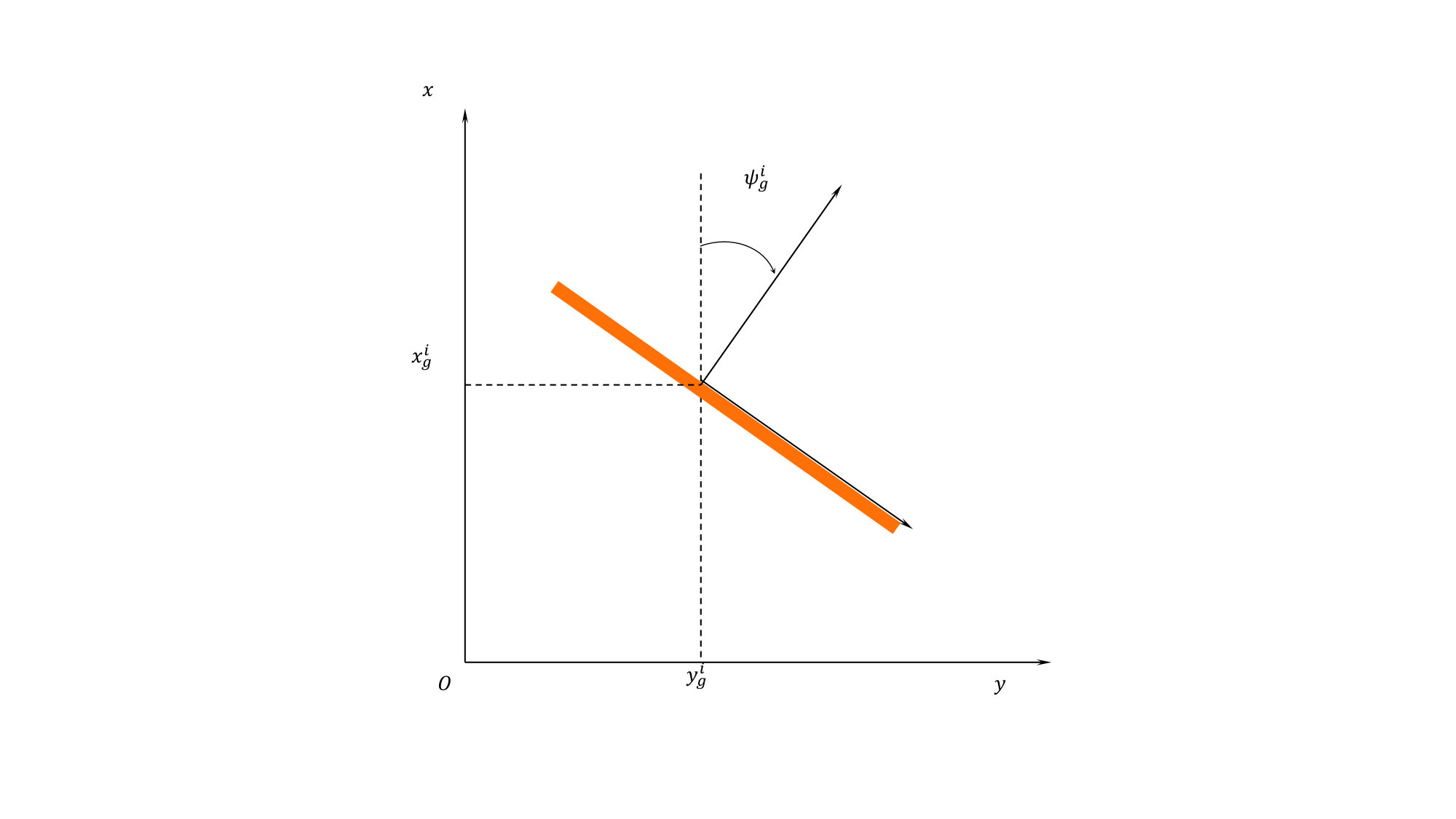 Figure 25
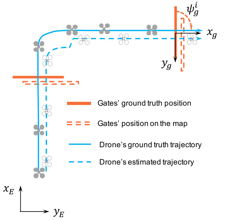 Figure 26
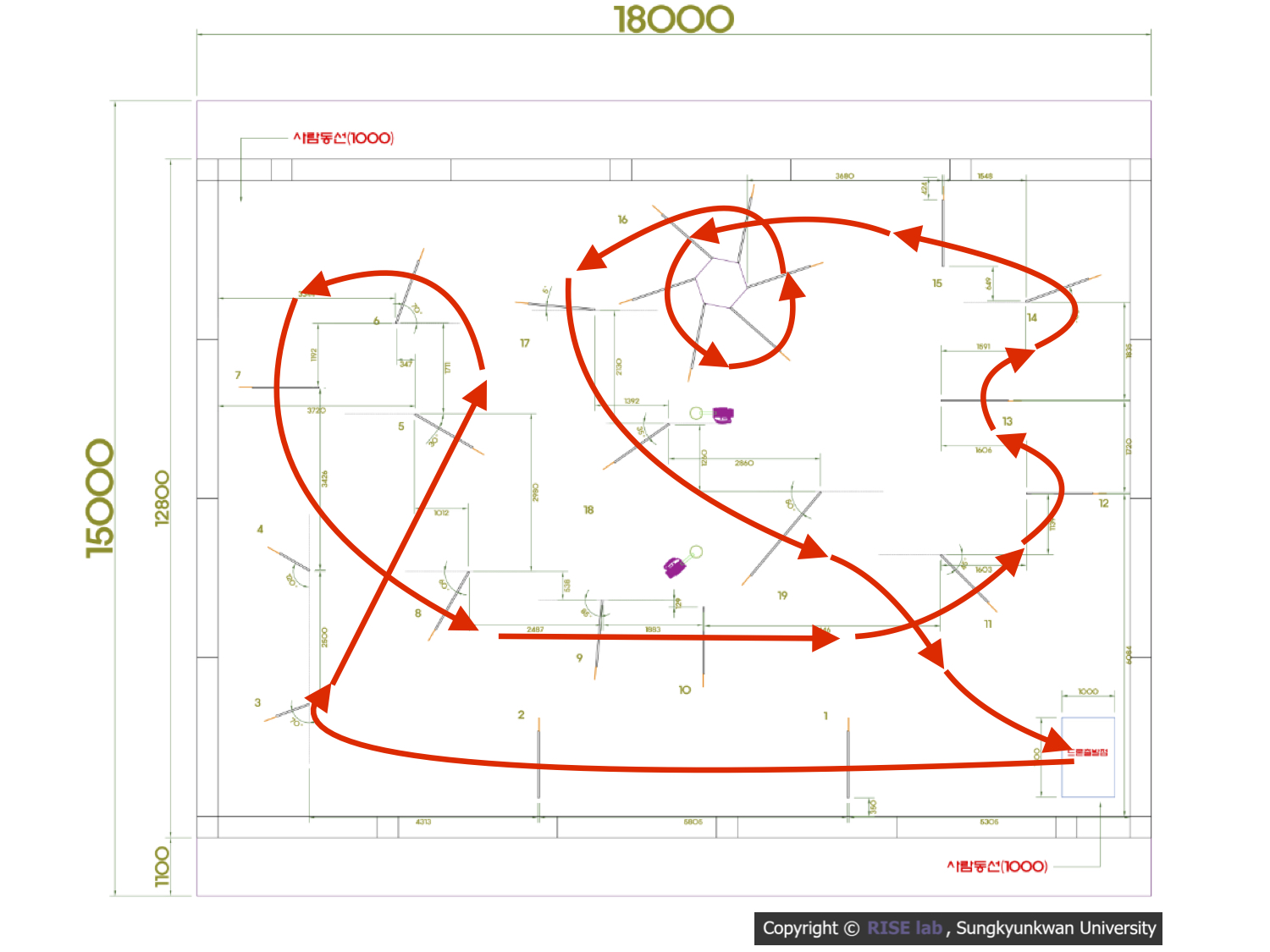 Figure 27
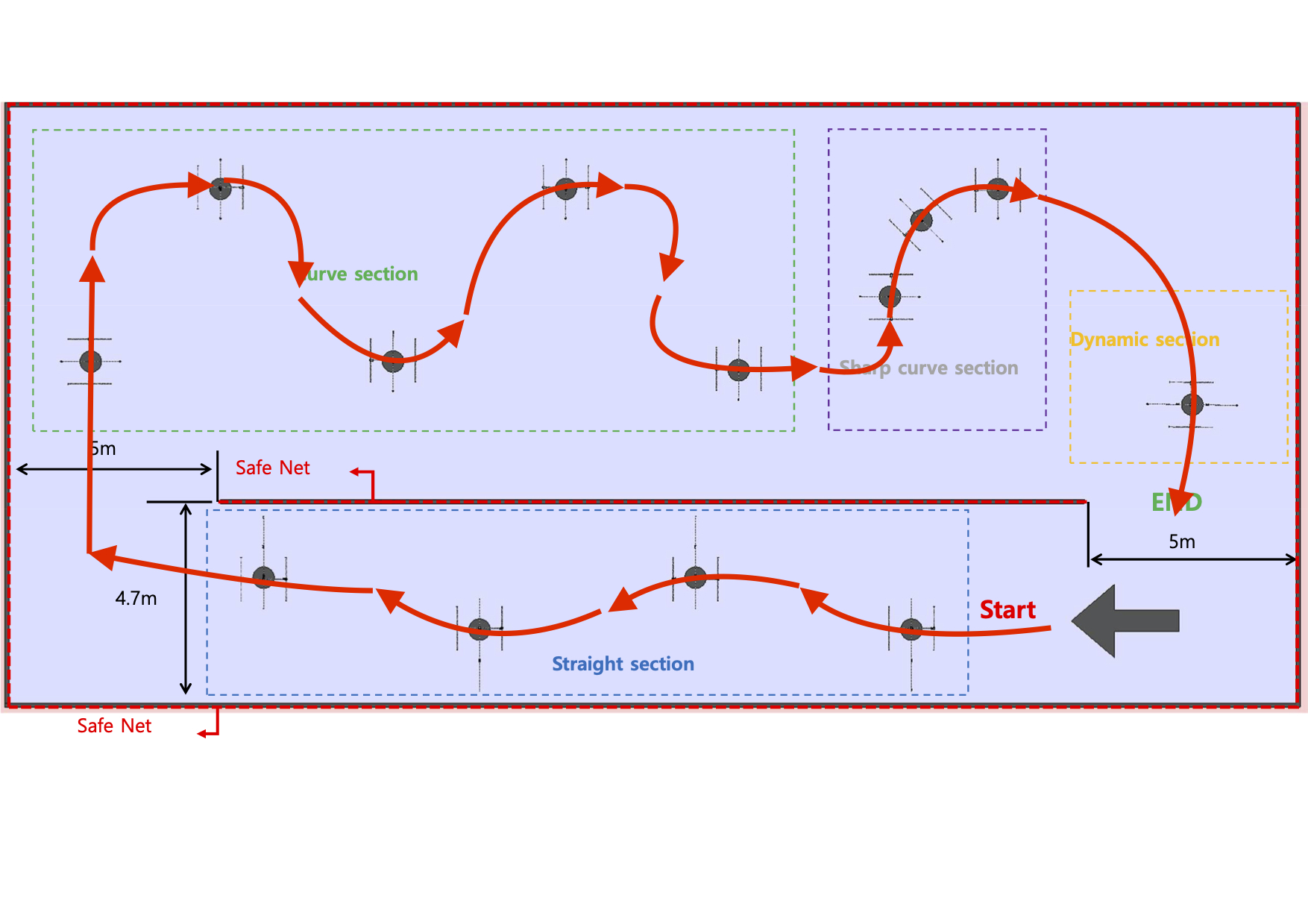 Figure 28
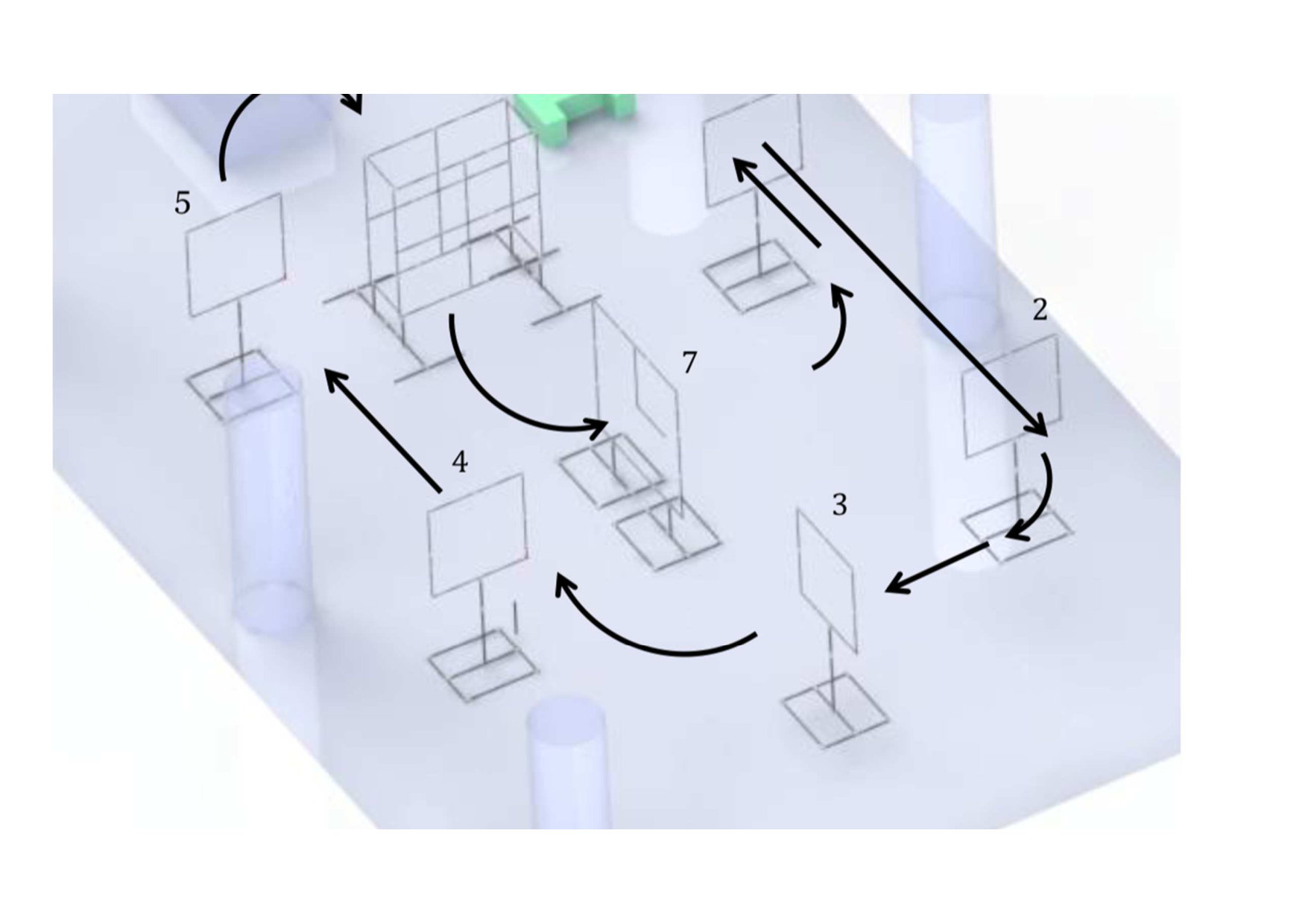 Figure 29
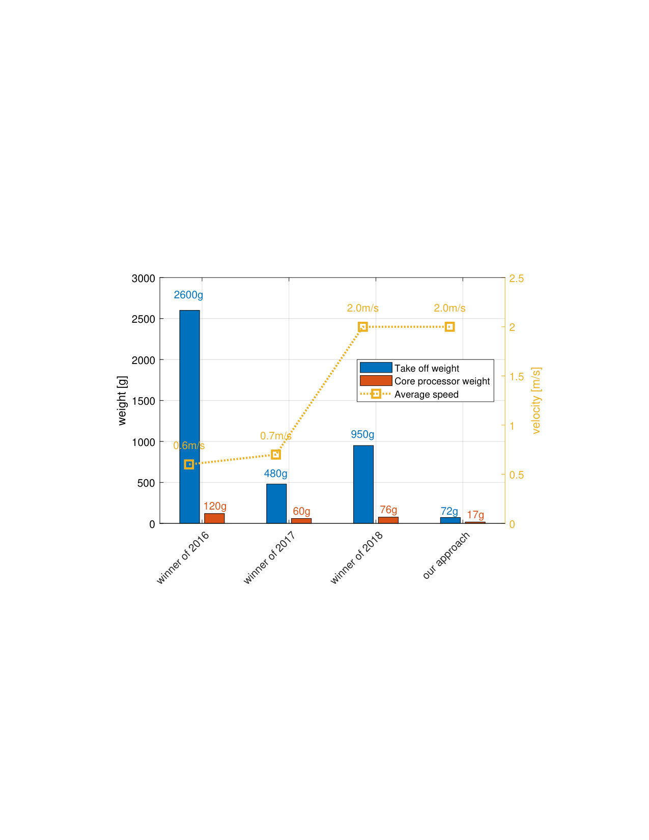 Figure 30
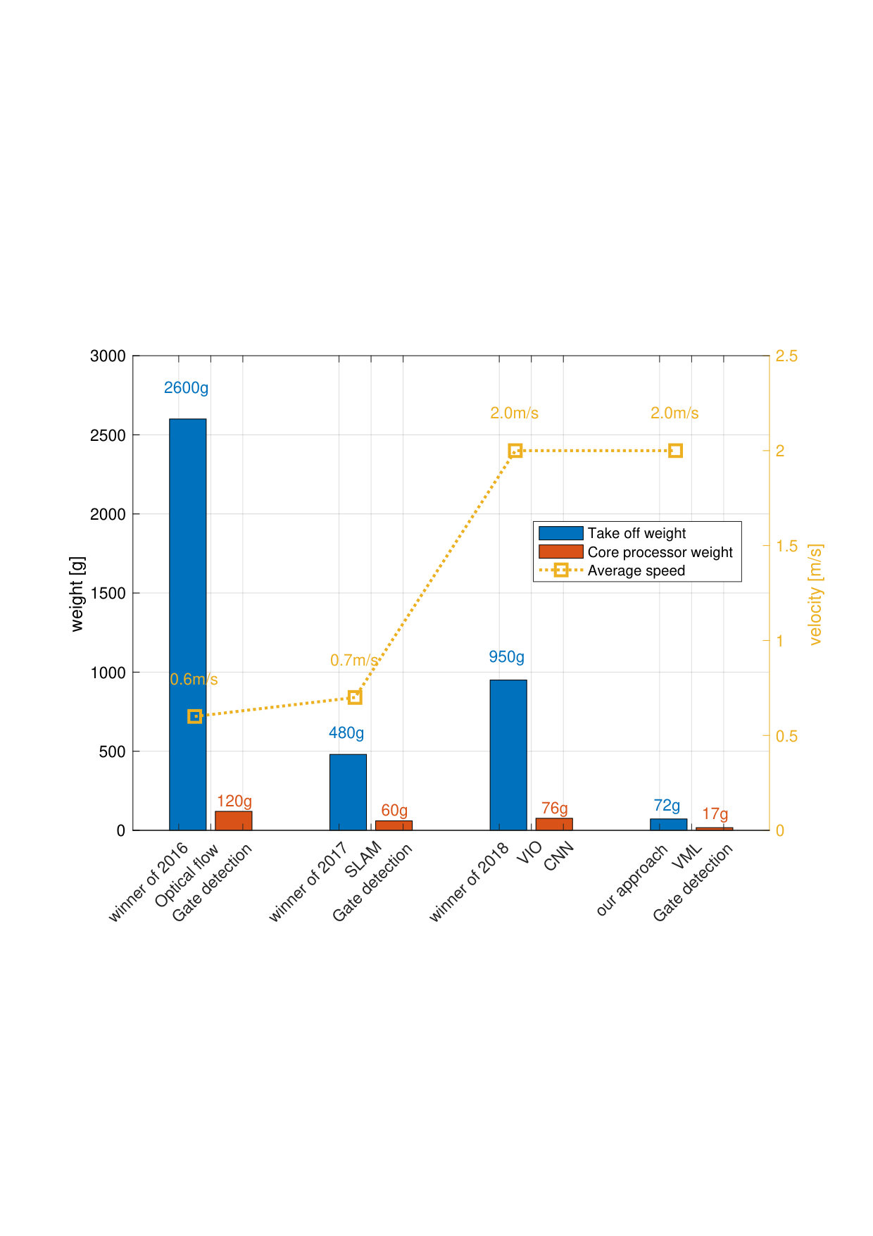 Figure 31
 Figure 32
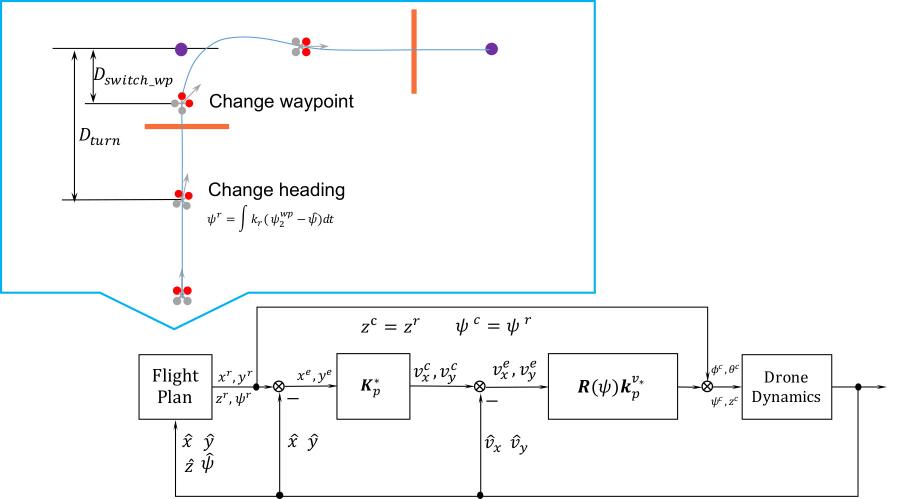 Figure 33
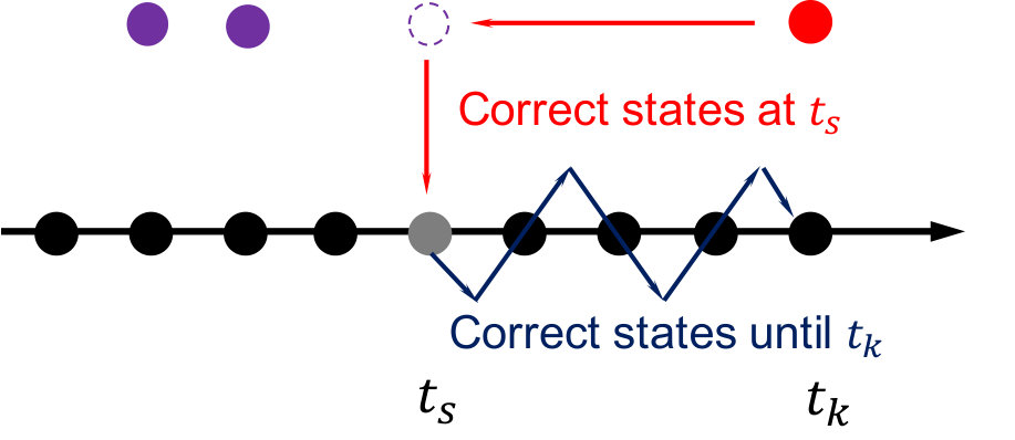 Figure 34
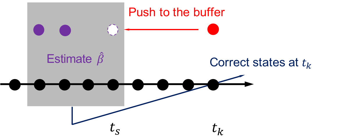 Figure 35
 Figure 36
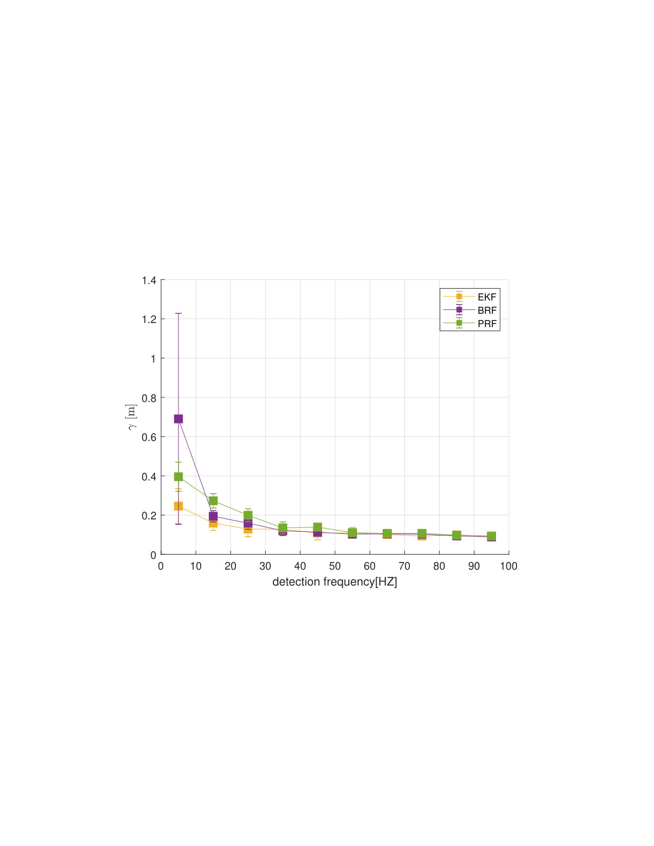 Figure 37
 Figure 38
 Figure 39
 Figure 40
| Weight | (with the original camera) |
|---|---|
| Size | |
| Motor | TC0803 KV15000 |
| MCU | STM32F4 (MHZ) |
| Receiver | FrSky D16 |
| Gate ID | ||||
|---|---|---|---|---|
| Snake gate detection (each image) | VML (each loop) | Controller (each loop) |
|---|---|---|
| gate ID | ||||
|---|---|---|---|---|
| 1 | 5 | 0 | 5 | 0 |
| 2 | 6.5 | 5 | 6.5 | 5 |
| 3 | 1 | 7 | 1 | 7 |
| 4 | 0 | 1 | 0 | 1 |
| gate ID | ||||
| 1 | 5 | 0 | 4 | 0 |
| 2 | 6.5 | 5 | 5 | 5 |
| 3 | 1 | 7 | 1 | 6 |
| 4 | 0 | 1 | 0 | 1 |
Peer Reviews
No public reviews on file for this paper yet. If you reviewed it on a platform where reviews are public (OpenReview, ICLR, NeurIPS, ICML), you can paste yours below so the community can read it here.
Videos
No videos yet. Explain this paper in a talk, walkthrough, or lecture? Add one.
Visual Model-predictive Localization for Computationally Efficient Autonomous Racing of a 72-gram Drone
Shuo Li
Micro Air Vehicle Lab
Delft University of Technology
Delft,The Netherlands, 2629HS 1
&Erik van der Horst
Micro Air Vehicle Lab
Delft University of Technology
Delft,The Netherlands, 2629HS 1
&Philipp Duernay
Delft University of Technology
Delft,The Netherlands, 2629HS 1
\ANDChristophe De Wagter
Micro Air Vehicle Lab
Delft University of Technology
Delft,The Netherlands, 2629HS 1
[email protected] &Guido C.H.E. de Croon
Micro Air Vehicle Lab
Delft University of Technology
Delft,The Netherlands, 2629HS 1
[email protected] ∗Corresponding author
Abstract
Drone racing is becoming a popular e-sport all over the world, and beating the best human drone race pilots has quickly become a new major challenge for artificial intelligence and robotics. In this paper, we propose a strategy for autonomous drone racing which is computationally more efficient than navigation methods like visual inertial odometry and simultaneous localization and mapping. This fast light-weight vision-based navigation algorithm estimates the position of the drone by fusing race gate detections with model dynamics predictions. Theoretical analysis and simulation results show the clear advantage compared to Kalman filtering when dealing with the relatively low frequency visual updates and occasional large outliers that occur in fast drone racing. Flight tests are performed on a tiny racing quadrotor named “Trashcan”, which was equipped with a Jevois smart-camera for a total of . The test track consists of laps around a 4-gate racing track. The gates are spaced meters apart and can be displaced from their supposed position. An average speed of is achieved while the maximum speed is . 111The video of the experiment is available at:
https://www.youtube.com/playlist?list=PL_KSX9GOn2P8H0QvUZtLZSYggzQ2DFHCi To the best of our knowledge, this flying platform is currently the smallest autonomous racing drone in the world and is times lighter than the existing lightest autonomous racing drone setup (), while still being one of the fastest autonomous racing drones.
1 Introduction
Drones, especially quadrotors, are transformed by enthusiasts in spectacular racing platforms. After years of development, drone racing has become a major e-sports, where the racers fly their drones in a preset course at high speed. It was reported that an experienced first person view (FPV) racer can achieve speeds up to when sufficient space is available. The quadrotor itself uses an inertial measurement unit (IMU) to determine its attitude and rotation rates, allowing it to execute the human’s steering commands. The human mostly looks at the images and provides the appropriate steering commands to fly through the track as fast as possible. The advance in research areas such as computer vision, artificial intelligence and control raises the question: would drones not be able to fly faster than human pilots if they flew completely by themselves? Until now, this is an open question. In 2016, the world’s first autonomous drone race was held at IROS 2016 [Moon et al., 2017], which became an annual event trying to answer this question (Figure 1).
We focus on developing computationally efficient algorithms and extremely light weight autonomous racing drones that have the same or even better performance than currently existing larger drones. We believe that these drones may be able to fly faster, as the gates will be relatively larger for them. Moreover, a cheap, light-weight solution to drone racing would allow many people to use autonomous drones for training their racing skills. When the autonomous racing drone becomes small enough, people may even practice with such drones in their own home.
Autonomous drone racing is indebted to earlier work on agile flight. Initially, quadrotors made agile maneuvers with the help of external motion capture systems [Mellinger and Kumar, 2011, Mellinger et al., 2012]. The most impressive feats involved passing at high speeds through gaps and circles. More recently, various researchers have focused on bringing the necessary state estimation for these maneuvers onboard. Loianno et al. plan an optimal trajectory through a narrow gap with difficult angles while using Visual Inertial Odometry (VIO) for navigation [Loianno et al., 2017]. The average maximum speed of their drone can achieve . However, the position of the gap is known accurately a priori, so no gap detection module is included in their research. Falanga et al. have their research on flying a drone through a gap aggressively by detecting the gap with fully onboard resources [Falanga et al., 2017]. They fuse the pose estimation from the detected gap and onboard sensors to estimate the state. In their experiment, the platform with a forward-facing fish-eye camera can fly through the gap with . Sanket et al. develop a solution for a drone to fly through arbitrarily shaped gaps without building an explicit 3D model of a scene, using only a monocular camera [Sanket et al., 2018].
Drone racing represents a larger, even more challenging problem than performing short agile flight maneuvers. The reasons for this are that: (1) all sensing and computing has to happen on board, (2) passing one gate is not enough. Drone races can contain complex trajectories through many gates, requiring good estimation and (optimal) control also on the longer term, and (3) depending on the race, gate positions can change, other obstacles than gates can be present, and the environment is much less controlled than an indoor motion tracking arena.
One category of strategies for autonomous drone racing is to have an accurate map of the track, where the gates have to be in the same place. One of the participants of the IROS 2017 autonomous drone race, the Robotics and Perception Group, reached gate in . In their approach, waypoints were set using the pre-defined map and VIO was used for navigation. A depth sensor was used for aligning the track reference system with the odometry reference system. NASA’s JPL lab report in their research results that their drone can finish their race track in a similar amount of time as a professional pilot. In their research, a visual-inertial localization and mapping system is used for navigation and an aggressive trajectory connecting waypoints is generated to finish the track [Morrell et al., 2018]. Gao et al. come up with a teach-and-repeat solution for drone racing [Gao et al., 2019]. In the teaching phase, the surrounding environment is reconstructed and a flight corridor is found. Then, the trajectory can be optimized within the corridor and be tracked during the repeating phase. In their research, VIO is employed for pose estimation and the speed can reach . However, this approach is sensitive to changing environments. When the position of the gate is changed, the drone has to learn the environment again.
The other category of strategies for autonomous drone race employs coarser maps and is more oriented on gate detection. This category is more robust to displacements of gates. The winner of IROS 2016 autonomous drone race, Unmanned Systems Research Group, uses a stereo camera for detecting the gates [Jung et al., 2018]. When the gate is detected, a waypoint will be placed in the center of the gate and a velocity command is generated to steer the drone to be aligned with the gate. The winner of the IROS 2017 autonomous drone race, the INAOE team, uses metric monocular SLAM for navigation. In their approach, the relative waypoints are set and the detection of the gates is used to correct the drift of the drone [Moon et al., 2019]. Li et al. combine gate detection with onboard IMU readings and a simplified drag model for navigation [Li et al., 2018]. With their approach, a Parrot Bebop 1 () can use its native onboard camera and processor to fly through gates with along a narrow track in a basement full of exhibits. Kaufmann et al. use a trained CNN to map the input images to the desired waypoint and the desired speed to approach it [Kaufmann et al., 2018b]. With the generated waypoint, a trajectory through the gate can be determined and executed while VIO is used for navigation. The winner of the IROS 2018 autonomous drone race, the Robotics and Perception Group, finished the track with [Kaufmann et al., 2018a]. During the flight, the relative position of the gates and a corresponding uncertainty measure are predicted by a Convolutional Neural Network (CNN). With the estimated position of the gate, the waypoints are generated, and a model predictive controller (MPC) is used to control the drone to fly through the waypoints while VIO is used for navigation.
From the research mentioned above, it can be seen that many of the strategies for autonomous drone racing are based on generic, but computationally relatively expensive navigation methods such as VIO or SLAM. These methods require heavier and more expensive processors and sensors, which leads to heavier and more expensive drone platforms. Forgoing these methods could lead to a considerable gain in computational effort, but raises the challenge of still obtaining fast and robust flight.
In this paper, we present a solution to this challenge. In particular, we propose a Visual Model-predictive Localization (VML) approach to autonomous drone racing. The approach does not use generic vision methods such as VIO and SLAM and is still robust to gate changes, while reaching speeds competitive to the currently fastest autonomous racing drones. The main idea is to rely as much as possible on a predictive model of the drone dynamics, while correcting the model and localizing the drone visually based on the detected gates and their supposed positions in the global map. To demonstrate the efficiency of our approach, we implement the proposed algorithms on a cheap, commercially available smart-camera called “Jevois” and mount it on the “Trashcan” racing drone. The modified Trashcan weighs only and is able to fly the race track with high speed (up to ). The vision-based navigation and high-level controller run on the Jevois camera while the low-level controller provided by the open source Paparazzi autopilot [Gati, 2013, Hattenberger et al., 2014] runs on the Trashcan. To the best of our knowledge, the presented drone is the smallest and one of the fastest autonomous racing drone in the world. Figure 2 shows the weight and the speed of our drone in comparison to the drones of the winners of the IROS autonomous drone races.
2 Problem Formulation and System Description
2.1 Problem Formulation
In this work, we will develop a hardware and a software system that the flying platform can fly through a drone race track fully autonomously with high speed using only onboard resources. The racing track setup can be changed and the system should be adaptive to this change autonomously.
For visual navigation, instead of using SLAM or VIO, we directly use a computationally efficient vision algorithm for the detection of the racing gate to provide the position information. However, implementing such a vision algorithm on low-grade vision and processing hardware results in low frequency, noisy detections with occasional outliers. Thus, a filter should be employed to still provide high frequency and accurate state estimation. In Section 3, we first briefly introduce the ’Snake Gate Detection’ method and a pose estimation method used to provide position measurements. Then, we propose and analyze the novel visual model-predictive localization technique that estimates the drone’s states within a time window. It fuses the low-frequency onboard gate detections and high-frequency onboard sensor readings to estimate the position and the velocity of the drone. The control strategy to steer the drone through the racing track is discussed. The simulation result in Section 4 shows the comparison between the proposed filter and the Kalman filter in different scenarios with outliers and delay. In Section 5, we will introduce the flying experiment of the drone flying through a racing track with gate displacement, different altitude and moving gate during the flight. In Section 6, the generalization and the limitation of the proposed method are discussed. Section 7 concludes the article.
2.2 System Overview
To illustrate the efficiency of our approach, we use a small racing drone called Trashcan (Figure 3). This racing drone is designed for FPV racing with the Betaflight flight controller software. In our case, to fly this Trashcan autonomously, we replaced Betaflight by the Paparazzi open source autopilot for its flexibility of adding custom code, stable communication with the ground for testing code and active maintenance from the research community. In this article, the Paparazzi software only aims to provide a low level controller. The main loop frequency is Hz. We employ a basic complementary filter for attitude estimation and the attitude control loop is a cascade control including a rate loop and an attitude loop. For each loop, a P-controller is used. The details of Trashcan’s hardware can be found in Table 1
For the high level vision, flight planning and control tasks, we use a light-weight smart camera () called Jevois, which is equipped with a quad core ARM Cortex A7 processor and a dual core Mali-400 GPU. In our experiment, there are two threads running on the Jevois, one of which is for vision detection and the other one is for filtering and control (Figure 4(a)). In our case, the frequency of detecting gates ranges from HZ to HZ and the frequency of filtering and control is set to HZ. The Gate detection thread processes the images in sequence. When it detects the gate it will send a signal telling the other thread a gate is detected. The control and filtering thread keeps predicting the states and calculating control command in high frequency. It uses a novel filtering method, explained in Section 3, for estimating the state based on the IMU and the gate detections.
The communication between the Jevois and Trashcan is based on the MAVLink protocol with a baud rate of . Trashcan sends the AHRS estimation with a frequency of HZ. And the Jevois sends the attitude and altitude commands to Trashcan with a frequency of HZ. The software architecture of the flying platform can be found in Figure 4(b).
In Figure 4(b), the Gate detection and Pose estimation module first detects the gate and estimates the relative position between the drone and the gate. Next, the relative position will be sent to the Gate assignment module to be transferred to global position. With the global position measurements and the onboard AHRS reading, the proposed VML filter fuses them together to have accurate position and velocity estimation. Then, the Flight plan and high level controller will calculate the desired attitude commands to steer the drone through the whole track. These attitude commands will be sent to the drone via MAVLink protocol. On the Trashcan drone, Paparazzi provides the low level controller to stabilize the drone.
3 Robust Visual Model-predictive Localization (VML) and Control
State estimation is an essential part of drones’ autonomous navigation. For outdoor flight, fusing a GPS signal with onboard inertial sensors is a common way to estimate the pose of the drone [Santana et al., 2015]. However, for indoor flight, a GPS signal is no longer available. Thus, off-board cameras [Lupashin et al., 2014], Ultra Wide Band Range beacons [Mueller et al., 2015] or onboard cameras [McGuire et al., 2017] can be used to provide the position or velocity measurements for the drone. The accuracy and time-delay of these types of infrastructure setups differ from each other. Hence, the different sensing setups have an effect on what type of filtering is best for each situation. The most commonly used state estimation technique in robotics is the Kalman filter and its variants, such as the Extended Kalman filter [Weiss et al., 2012, Santamaria-Navarro et al., 2018, Gross et al., 2012]. However, the racing scenario has properties that make it challenging for a Kalman filter. Position measurements from gate detections often are subject to outliers, have non-Gaussian noise, and can arrive at a low frequency. This makes the typical Kalman filter approach unsuitable because it is sensitive to outliers, is optimal only for Gaussian noise, and can converge slowly when few measurements arrive. In this section, we will propose a visual model-predictive localization technique which is robust to low-frequency measurements with significant numbers of outliers. Subsequently, we will also present the control strategy for the autonomous drone race.
3.1 Gate assignment
In this article, we use the “snake gate detection” and pose estimation technique as in Li et al. [Li et al., 2018]. The basic idea of snake gate detection is searching for continuing pixels with the target color to find the four corners of the gate. Subsequently, a perspective -point (PnP) problem is solved, using the position of the four corners in the image plane, the camera’s intrinsic parameters, and the attitude estimation to solve the relative position between the drone and the gate at time , . Figure 5 shows this procedure, which is explained more in detail in [Li et al., 2018]. In most cases, when the light is even and the camera’s auto exposure works properly, the gate in the image is continuous and the Snake gate detection algorithm can detect the gate correctly. However, after an aggressive turn, such as a turn to a window, the camera cannot adapt to the new light condition immediately. In this case, Snake gate detection usually cannot detect the gate. Another failure case is that due to the uneven light condition or the similar color in the background, Snake gate detection may get interfered with. These situations make the searching stop in the middle of the bar or stop at the background pixels. Although we have some mechanism to prevent these false positive detections, there is still a small chance that a false positive happens. The negative effect is that outliers may appear which leads to a challenge for the filter and the controller.
Since for any race a coarse map of the gates is given a priori (cf. Figure 1), the position and the heading of gate , can be known roughly (Figure 6). We use the gates’ positions to transfer the relative position measured by camera to a global position by equation 1. In equation 1, , and are the position of the gate which are known from the map.
[TABLE]
Here, we assume that the position of the gate is fixed. Any error experienced in the observations is then assumed to be due to estimation drift on the part of the drone. Namely, without generic VIO, it is difficult to make the difference between drone drift and gate displacements. If the displacements of the gates are moderate, this approach will work: after passing a displaced gate, the drone will see the next gate, and correct its position again. We only need a very rough map with the supposed global positions of the gates (Figure 6). Gate displacements only become problematic if after passing gate the gate would not be visible when following the path from the expected positions of gate to gate .
At the IROS drone race, gates are identical, so for our position to be estimated well, we need to assign a detection to the right gate. For this, we rely on our current estimated global position . When a gate is detected, we go through all the gates on the map using equation 1 to calculate the predicted position . Then, we calculate the distance between the predicted drone’s position and its estimated position at time by
[TABLE]
After going through all the gates, the gate with the predicted position closest to the estimated drone position is considered as the detected gate. At time , the measurement position is determined by
[TABLE]
The gate assignment technique can help us obtain as much information on the drone’s position as possible when a gate is detected. Namely, it can also use detections of other gates than the next gate, and allows to use multiple gate detections at the same time in order to improve the estimation. Still, this procedure will always output a global coordinate for any detection. Hence, false positive or inaccurate detections can occur and have to be dealt with by the state estimation filter.
3.2 Visual Model-predictive Localization (VML)
The racing drone envisaged in this article has a forward-looking camera and an Inertial Measurement Unit (IMU). As explained in the previous section, the camera is used for localization in the environment, with the help of gate detections. Using a typical, cheap CMOS camera will result in relatively slow position updates from the gate detection, with occasional outliers. The IMU can provide high-frequency, and quite accurate attitude estimation by means of an Attitude and Heading Reference System (AHRS). The accelerations can also be used in predicting the change in translational velocities of the drone. In traditional inertial approaches, the accelerations would be integrated. However, for smaller drones the accelerometer readings become increasingly noisy, due to less possible damping of the autopilot. Integrating accelerometers is ‘acceleration stable’, meaning that a bias in the accelerometers that is not accounted for can lead to unbounded velocity estimates. Another option is to use the accelerometers to measure the drag on the frame, which - assuming no wind - can be easily mapped to the drone’s translational velocity (cf. [Li et al., 2018]). Such a setup is ‘velocity stable’, meaning that an accelerometer offset of drag model error would lead to a proportional velocity offset, which is bounded. On really small vehicles like the one we will use in the experiments, the accelerometers are even too noisy for reliably measuring the drag. Hence, the proposed approach uses a prediction model that only relies on the attitude estimated by the AHRS which is an indirect way of using the accelerometer. It uses the attitude and a constant altitude assumption to predict the forward acceleration, and subsequently velocity of the drone. The model is corrected from time to time by means of the visual localization. Although the IMU is used for estimating attitude, it is not used as an inertial measurement for updating translational velocities. This leads to the name of the method; Visual Model-predictive Localization (VML), which will be explained in detail in this subsection.
3.2.1 Prediction Error Model
As mentioned above, the attitude estimated from the AHRS is used in the prediction of the drone’s velocity and position. However, due to the AHRS bias and the model inaccuracy, the prediction will diverge from the ground truth over time. Fortunately, we have visual gate detections to provide position information. This vision-based localization will not integrate the error over time but it has a low frequency. Figure 8 is a sketch of what the onboard predictions and the vision measurements look like. The red curve is the prediction result diverging from the ground truth curve because of AHRS biases. The magenta dots are the low frequency detections which distribute around the ground truth. The error between the prediction and measurements can be modeled as a linear function of time which will be explained later in this section. When the error model is estimated correctly, it can be used to compensate for the divergence of the prediction to obtain accurate state estimation.
Assuming that there is no wind, and knowing the attitude, we can predict the acceleration in the and axis. Figure 9 shows the forces the drone experiences. denotes the acceleration caused by the thrust of the drone. It provides the forward acceleration together with the pitch angle . denotes the acceleration caused by the drag which is simplified as a linear function of body velocity. [Faessler et al., 2017]
[TABLE]
where is the drag coefficient.
According to Newton’s second law in plane,
[TABLE]
Expand equation 5, we have
[TABLE]
where is the rotation matrix and is the drag coefficient matrix. If the altitude is kept the same as in the IROS drone race, we have
[TABLE]
Since the model in the axis has the same form as in the axis, the dynamic model of the quadrotor can be simplified as
[TABLE]
where and are the position of the drone, and is the roll angle of the drone. In equation 8, the movement in and axis is decoupled. Thus we only analyze the movement in the axis. The result can be directly generalized to the axis. The nominal model of the drone in axis can be written by
[TABLE]
where ,, and . The superscript denotes the nominal model. Similarly, with the assumption that the drag factor is accurate, the prediction model can be written as
[TABLE]
where and . is the AHRS bias and is assumed to be a constant in short time. Consider a time window , the states of nominal model at time are
[TABLE]
where is the sampling time. The predicted states of model 10 are
[TABLE]
Thus, the error between the predicted model and nominal model can be written as
[TABLE]
where is the input bias which can be considered as a constant in a short time. In equation 13,
[TABLE]
Since the sampling time is small, ( in our case), we can assume
[TABLE]
Hence, equation 13 can be approximated by
[TABLE]
Expanding equation 17, we have
[TABLE]
Actually, is the time span of the time window. If we neglect term, we can have the prediction error at time
[TABLE]
Thus, within a time window, the state estimation problem can be transformed to a linear regression problem with model equation 19, where are the parameters to be estimated. From equation 19, we can see that in a short time window, the AHRS bias does not affect the prediction error. The error is mainly caused by the initial prediction error . Furthermore, velocity error can cause the prediction error to diverge over time. If the time window is updated frequently, model 19 can remain accurate enough. Hence, in this work, we focus on the main contributors to the prediction error and will not estimate the bias term. The next step is how to efficiently and robustly estimate and .
In this simplified linear prediction error model, we use the constant altitude assumption to approximate the thrust on the drone, which may lead to inaccuracy of the model. During the flight, this assumption may be violated by aggressive maneuvers in axis. However, if the maneuver in axis is not very aggressive and the time window is small (in our case less than ), the prediction error model’s inaccuracy level can be kept in an acceptable range. In the simulation and the real-world experiment shown later, we will show that although the altitude of the drone changes in , the proposed filter can still have very high accuracy with this assumption. Another way to improve the model accuracy is to estimate the thrust by fusing the accelerometer readings and rotor speed together, which needs the establishment of the rotors’ model. It should also be noted that we neglect term in equation 18 to have a linear model. To increase the model accuracy, the prediction error model can be a quadratic model. In our case, since the time window is small, the linear model is accurate enough.
3.2.2 Parameter Estimation Method
The classic way for solving the linear regression problem based on equation 19 is to use the Least Square Method (LS Method) with all data within the time window and estimate the parameters .
[TABLE]
where
[TABLE]
The LS Method in equation 20 can give optimal unbiased estimation. However, if there exist outliers in the time window , they will be considered equally during the estimation process. These outliers can significantly affect the estimation result. Thus, to exclude the outliers, we employ random sample consensus (RANSAC) to increase the performance [Fischler and Bolles, 1981]. In a time window , we first calculate the prediction error and time difference . For each iteration , the subsets of and are randomly selected, which are denoted by and . The size of the subset can be calculated by , where is the ratio of sampling. We use subsets and to estimate the parameters (Figure 10).
When is estimated, it will be used to calculate the total prediction error of the all the data in the time window by
[TABLE]
where
[TABLE]
In the process of equation 21, if is larger than a threshold , it counts the threshold as the error. After all the iterations, the parameters which has the least prediction error will be selected to be the estimated parameters for this time window . The pseudo-code of this Basic RANSAC Fitting (BRF) method can be found in Algorithm .
With the Basic RANSAC Fitting (BRF) method, the influence of the outliers is reduced, but it has no mechanism to handle over-fitting. For example, in time window , BRF can estimate the optimal parameters with the minimal error. However, sometimes it will set to unrealistically high values. This happens when there are few detections in the time window, which may result in the inaccurate estimation of the parameters. In reality, the drone flies at maximum speed , so the velocity prediction error at the start of time window should not be too large. To avoid over-fitting, we add a penalty factor/prior matrix to limit in the fitting process. The loss function can be written as
[TABLE]
where
[TABLE]
is the penalty factor/prior matrix. To minimize the loss function, we take derivatives of and let it be [math]
[TABLE]
Then we have the estimated parameters by
[TABLE]
We call the use of equation 28 inside the RANSAC fitting the Prior RANSAC fitting (PRF). Compared to equation 20, PRF has the penalty factor/prior matrix in it. By tuning matrix we can add the prior knowledge to the parameter distribution. For example, in our case should not be high. Thus, we can increase in to limit the value of .
To conclude, in this part we propose methods for estimating the parameters . The first one is the LS Method which considers all the data in a time window equally. The second method is Basic RANSAC Fitting method (BRF), which has the mechanism to exclude the outliers. And the third one is Prior RANSAC Fitting method (PRF), which can not only exclude the outliers but also take into account the prior knowledge to avoid over-fitting. In the next section, we will discuss and compare these methods in simulation to see which one is the most suitable for our drone race scenario.
3.2.3 Prediction Compensation
After the error model (equation 19) is estimated in time window , the error model can be used to compensate the prediction by
[TABLE]
Also, at each prediction step, the length of the time window will be checked, since the simplified model 19 is based on the assumption that the time span of the time window is small. If is larger than the allowed maximum time window size , the filter will delete the oldest elements until . The pseudo-code of the proposed VML with LS Method can be found in Algorithm and Algorithm .
3.2.4 Comparison with Kalman Filter
When it comes to state estimation or filtering technique, it is inevitable to mention the Kalman filter which is the most commonly used state estimation method. The basic idea of the Kalman filter is that at time , it first predicts the states at time with its error covariance to have prior knowledge of the states at .
[TABLE]
When an observation arrives, the Kalman filter uses an optimal gain which is a combination of the prior error covariance and the observation’s covariance to compensate the prediction, which as a result, leads to the minimum error covariance .
[TABLE]
According to [Diderrich, 1985], a Kalman filter is a least square estimation made into a recursive process by combining prior data with coming measurement data. The most obvious difference between the Kalman filter and the proposed VML is that VML is not a recursive method. It does not estimate the states at only based on the last step states . It estimates the states considering the previous prediction and observations in a time window.
In the VML approach, we use least square method within a time window, which looks similar to the least square estimation method. However, there are two major differences between the two methods. The first one is that in the proposed VML, the prediction information is fused to the VML. Secondly and most importantly, we estimate the prediction error model instead of estimating all the states in the time window as in the least square method. Thus, the VML has its advantages of handling outliers and delay by its time window mechanism and it also has the advantage of computational efficiency to the Least Square Estimation. In Section 4, we will introduce Kalman filter’s different variants for outliers and delay and compare them with VML in estimation accuracy and computation load in detail.
3.3 Flight Plan and High Level Control
With the state estimation method explained above, to fly a racing track, we employ a flight plan module which sets the waypoints that guide the drone through the track and a two-loop cascade P-controller to execute the reference trajectory (Figure 11).
Usually, the waypoint is just behind the gate. When the distance between the drone and the waypoint is less than a threshold , the gate can no longer be detected by our method, and we set the heading of the drone to the next waypoint. This way, the drone will start turning towards the next gate before arriving at the waypoint. When the distance between the drone and the waypoint is within another threshold , the waypoint switches to the next point. With this strategy, the drone will not stop at one waypoint but already start accelerating to the next waypoint, which can help to save time. The work flow of flight plan module can be found in Algorithm .
We employ a two-loop cascade P controller (equation 32) to control the drone to reach the waypoints and follow the heading reference generated from the flight plan module. The altitude and attitude controllers are provided by the Paparazzi autopilot, and are both two-loop cascade controllers.
[TABLE]
where , , , , , , .
4 Simulation Experiments
4.1 Simulation Setup
To verify the performance of VML in the drone race scenario, we first test it in simulation and then use an Extended Kalman filter as benchmark to compare both filters to see which one is more suitable in different operation points. We first introduce the drone’s dynamics model used in the simulation.
[TABLE]
where is the position of the drone in the Earth frame. is the velocity of the drone. is the gravity factor. is the acceleration caused by the thrust force. , , are the three Euler angles of the body frame. And is the rotation matrix from the Body frame to the Earth frame. is the simplified first order drag matrix, where the values are based on a linear fit of the drag based on real-world data with the Trashcan drone. is the acceleration caused by other aerodynamics. The last four equations are the simplified first order model of the attitude controller and thrust controllers where the proportional feedback factors are , ,,. Thus, the model 33 in the simulation is a states and inputs nonlinear system. In this simulation, we use the same flight plan module and high-level controllers discussed in Section 3 (Figure 11) to generate a ground truth trajectory through a 4-gate square racing track. In this track, we use different height to test if the altitude change affects the accuracy of the VML.
With the ground truth states, next step is to generate the sensor reading. In the real world, AHRS estimation outputs biased attitude estimation because of the accelerator’s bias. To model AHRS bias, we have a simplified AHRS bias model
[TABLE]
where and are the AHRS biases on and . and are the north and east bias caused by the accelerometer bias, which can be considered as constants in short time. From real-world experiments, they are less than . Thus, the AHRS reading can be modelled by
[TABLE]
where is the AHRS noise and in our simulation we will set , , . For vision measurements generation, we first determine the segment of the trajectory where the drone can detect the gate. Then, we calculate the number of the detection by , where is the detection frequency. Next, we randomly select points between and to be vision points. For these points, we generate detection measurement by
[TABLE]
In equation 36, is the detection noise and In these vision points, we also randomly select a few points as outlier points, which have the same model with equation 36 but . In the following simulations, the parameters are the same with the value mentioned in this section if there is no statement. The simulated ground truth states and sensor measurements are shown in Figure 12(b).
4.2 Simulation result and analysis
4.2.1 Comparison between EKF, BRF and PRF without outliers
We employ an EKF as benchmarks to compare the performance of our proposed filter. The details of the EKF can be found in the Appendix. We first do the simulation in only one operation point, where HZ, and the probability of outliers . At this operation point, three filters are run separately. The result is shown in Figure 13.
When there are no outliers, all three filters can converge to the ground truth value. However, the EKF has a longer startup period and BRF overfits after turning, leading to unlikely high velocity offsets (the peaks in Figure 13b)). This is because, after the turn, the RANSAC buffer is empty. When the first few detections come into the buffer, the RANSAC has a larger chance to estimate inaccurate parameters. In PRF, however, we add a prior matrix to limit the value of and the number of the peaks in the velocity estimation is significantly decreased. At the same time, the velocity estimation is closer to the ground truth value.
To evaluate the estimation accuracy of each filter, we first introduce a variable, average estimation error , to be an index of the filter’s performance:
[TABLE]
where is the number of the sample points on the whole trajectory. and are the estimated states by the filter. and are the ground truth positions generated by the simulation. captures how much the estimated states deviate from the ground truth states. A smaller indicates a better filtering result.
We use running time to evaluate the computation efficiency of each filter. It should be noted that since we need to store all the simulation data for visualization and MATLAB has no mechanism of passing pointers, data accessing can take much computation time. Thus, we only count the running time of the core parts of the filters, which are the prediction and the correction.
The results are shown in Figure 14. In the simulation, the time-window in BRF and PRF is set to be and iterations are performed in the RANSAC procedure. For each frequency, the filters are run times separately and their average and running time are calculated. It can be seen in Figure 14(a) that when the detection frequency is larger than HZ, BRF and PRF perform close to the EKF. In terms of calculation time, the EKF is heavier than BRF and PRF when the frequency is lower than . It is because that during the prediction phase, the EKF not only predicts the states but also calculates the Jacobian matrix and the prior error covariance by high frequency while BRF and PRF only do the state prediction. However, when the detection comes, the EKF does the correction by several matrix operations while BRF and PRF do the RANSAC which is much heavier. This explains why the EKF’s computation load is only slightly affected by the detection frequency but BRF and PRF’s computation load increases significantly with higher detection frequency.
4.2.2 Comparison between EKF, BRF and PRF with outliers
When outliers appear, the regular EKF can be affected significantly. Thus, outlier rejection strategies are always used within an EKF to increase its robustness. A commonly used method is using Mahalanobis distance between the observation and its mean as an index to determine whether an observation is an outlier. [Chang, 2014, Li et al., 2016] Thus, in this section, we implement an EKF with outlier rejection (EKF-OR) as a benchmark to compare the outlier rejection performance of BRF and PRF. The basic idea for the EKF-OR is that the square of the observation’s Mahalanobis distance is Chi-square distributed. Hence, when the observation arrives, its Mahalanobis distance will be calculated and checked whether it is within a threshold . If it is not, this observation will be rejected.
Two examples of the filters’ rejecting outliers are shown in Figure 15. The first figure shows a common case that the three filters can reject the outliers successfully. However, in some special cases, EKF-OR is vulnerable to the outliers. In Figure 15(b), for instance, after a long time of pure prediction, the error covariance becomes large. Once EKF-OR meets an outlier, it has a high chance to jump to it. The subsequent true positive detections will be treated as outliers and EKF-OR starts diverging. At the same time, BRF and PRF are more robust to the outliers. The essential reason is that for EKF-OR, it depends on its current state estimation (mean and error covariance) to identify the outliers. When the current state estimation is not accurate enough, like the long-time prediction in our case, EKF-OR loses its ability to identify outliers. In other words, it tends to trust whatever it meets. The worse situation is that after jumping to the outlier, its error covariance become smaller which, as a consequence, leads to the rejection of the coming true positive detections. However, for BRF and PRF, outliers are determined in a time window including history. Thus, after long time of prediction, when BRF and PRF meet an outlier, they will judge it considering the detections in the past. If there is no other detection in the time window, they will wait for enough detections to make a decision. With this mechanism, BRF and PRF become more robust than EKF-OR especially when EKF-OR’s estimation is not accurate.
Figure 16 shows the estimation error and the calculation time of the three filters. As we stated before, although EKF-OR has the mechanism of dealing with the outliers, it still can diverge due to the outliers in some special cases. Thus, in Figure 16(a) EKF-OR has large estimation error when the detection frequency is both low and high. In terms of calculation time, it can be seen that it has no significant difference with the non-outlier case.
4.2.3 Filtering result with delayed detection
Image processing and visual algorithms can be very computationally expensive for running onboard a drone, which can lead to significant delay. [van Horssen et al., 2019, Weiss et al., 2012] Many visual navigation approaches ignore this delay and directly fuse the visual measurements with the onboard sensors, which sacrifices the accuracy of the state estimation. A commonly used approach for compensating this vision delay is a modified Kalman filter proposed by Weiss et al. [Weiss et al., 2012]. The main idea of this approach, called EKF delay handler (EKF-DH), is having a buffer to store all sensor measurements within a certain time. At time , a vision measurement corresponding to the states at earlier time arrives. It will be used to correct the states at time . Then, the states will be propagated again from to . (Figure 17(a)) Although updating the covariance matrix is not needed according to [Weiss et al., 2012], this approach still requires updating history states whenever a measurement arrives, which can be computationally expensive especially when the delay and the measurement frequency get larger. In our case, we need to use the error covariance for outlier rejections, it is necessary to update the history error covariance matrices, which in turn increases the computation load further. At the same time, for VML, when the measurement arrives, it will first be pushed into the buffer. Then, the error model will be estimated within the buffer/time window. With the estimated parameter , the prediction at can be corrected directly without the need of correcting all the states between and . (Figure 17(b)) Thus, the computational burden will not increase when the delay exists.
Figure 18 shows an example of the simulation result of the three filters when both outliers and delay exist. In this simulation, the visual delay is set to be . It can be seen that although there is a lag between the vision measurements and the ground-truth, all the filters can estimate accurate states. However, EKF-DH requires much more computation effort. Figure 19 shows the estimation error and the computation time of the three filters.
In Figure 19, we can see that the computation load of EKF-DH increases significantly due to its mechanism of handling delay. Unsurprisingly, EKF-DH is still sensitive to some outliers while BRF and PRF can handle the outliers.
5 Real-world Experiments
5.1 Processing time of each component
Before testing the whole system, we first test on the ground how much time the Snake gate detection, the VML and the controller take when running on a Jevois smart camera. On the ground, we set an orange gate in front of a Jevois camera and calculate the time that each component takes. For each image, we start timing when a new image arrives and the Snake gate detection is run. Then, we stop timing when the snake gate finishes. For VML, in each loop, the timing includes both prediction and correction no matter if there are enough detections for correction. We start counting when the Jevois is powered on. In this test, the vision detection frequency is and the number of RANSAC iterations in VML is set to . Table 3 shows the statistical results of the time each component takes on the Jevois.
From Table 3, it can be seen that vision takes much more time than the other two parts. Please note though that the snake gate computer vision detection algorithm is already a very efficient gate detection algorithm. In fact, it has tunable parameters, i.e., the number of samples taken per image for the detection (3000 in the current setup), which allow the algorithm to run even much faster at the cost of having less accuracy (see [Li et al., 2018] for more details). The main gain in time in the approach presented in this article is that we do not employ VIO and SLAM, which would take substantially more processing. However, as the Snake gate detection provides relatively low-frequency and noisy position measurements, the VML needs to run in high frequency and cope with the detection noise to still provide accurate estimation for the controller.
5.2 Flying experiment without gate displacement
Figure 21 shows the flying result of the drone flying the track without gate displacement. The position of the gates is listed in Table 4. In Table 4, and are the position of the gates in the real world and and are their position on the map. In this situation, they are the same. The aim of this experiment is to test the filter’s performance with sufficient detections. Thus, the velocity is set to be to give the drone more time to detect the gate. In Figure 21, the blue curve is the ground truth data from Optitrack motion capture system and the yellow curves are the filtering results. From the flying result, it can be seen that the filtered results are smooth and coincide with the ground truth position well. During the period when the detections are not available, the state prediction is still accurate enough to navigate the drone to the next gate. When the drone detects the next gate, the filter will correct the prediction. In this situation, the divergence of the states is only caused by the prediction drift. It should also be noted that when the outliers appears at , the filter is not affected by them because of the RANSAC technique in the filter. The processing time of the visual detection, the filter and the controller are listed in Table 3. It can be seen that the VML proposed in this article is extremely efficient.
5.3 Flying experiment with gate displacement
In this section, we test our strategy under a difficult condition where the drone flies faster, the gates are displaced and the detection frequency is low. The real gate positions and their position on the map are listed in Table 5 and shown in Figure 22(a). Gates are displaced between 0 and 1.5m from their supposed positions. The dashed orange lines in Figure 22(a) denote the gate positions on the map while the solid orange lines denote the real gate positions which are displaced from the map. Figure 22(b) shows the flight data of the first lap. The orange solid gates are the ground truth positions of the gates. The yellow curve is the filtered position based on the gates’ positions on the map (orange dashed gates). In other words, the yellow curve is where the drone thinks it is based on the knowledge of the map. After passing through one gate, when the drone detects the next gate, the filter will start correcting the filtering error from the prediction error and the gate displacement.
The whole flight result is shown in Figure 23. From the result, it can be seen that the drone can fly the track for laps with an average speed of and a maximum speed of while an experienced pilot flies the same drone in the same track with an average speed of after several runs of training. Figure 23(a) is the filtering result of the position. It should be noted that the filtering result does not coincide with the ground truth curve because of the displacement of the gates. The pose estimation is based on the gates’ position on the map. When the gates are displaced, the drone still thinks they are at the position which the map indicates. After the turn, when the drone sees the next gate, which is displaced, it will attribute the misalignment to the prediction error and correct the prediction by means of new detections. With this strategy, our algorithm is robust to the displacement of the gates.
5.4 Flying experiment with different altitude and moving gate
We also show a more challenging trace track where the height of the gates varies from to . Also, during the flight, the position of the second gate () is changed after the drone passes through it. In the next lap, the drone can adapt to the changing position of the gate. (Figure 24)
The flight result is shown in Figure 25. In this flight, the waypoints are not changed and the gates are deployed without any ground truth measurement. Thus, the estimated position does not coincide with the ground-truth position. It should be noted that the height difference between the second gate and the third gate is . With this altitude change which violates the constant altitude assumption for the prediction error model, the proposed VML is still accurate enough to navigate the drone through the gate.
From the real flight result, we can see that the VML performs well and can navigate the drone through the racing track with high speed even though the gates are displaced. Also, this strategy does not need computationally expensive methods like generic VIO and SLAM. This allows it to be run on a very light-weight flying platform.
6 Discussion
In this paper, we proposed a novel state estimation method called Visual Model-predictive Localization which provides navigation information for a 72 gram autonomous racing drone. The algorithm’s properties were thoroughly studied in simulation and the feasibility of real-world implementation was shown in challenging real world experiments. Although in this paper VML is used for a specific drone race scenario, this method can be directly used for navigation in other more general scenarios where the sensors have low frequency, temporary failure, outliers and delays. For example, our approach can be directly adopted into an outdoor environment where position measurements are provided by a GPS signal that has a delay, temporary failures and outliers. Just as in our drone race experiments, the proposed approach should be more reliable than a Kalman filter. For indoor flight, we used a common linear drag model for state prediction which does not need a lot of effort and precise equipment to identify. Outdoor flight would require adaptations to this model, for instance such as the ones explained in, e.g., [Sikkel et al., 2016].
We implemented our approach by adding a cheap smart camera Jevois to a tiny racing drone Trashcan. With very limited carrying capacity and more complex aerodynamics property, it is still demonstrated that this light-weight flying platform has the ability to finish the drone race task autonomously. Compared to a regular size racing drone, the Trashcan has more complex aerodynamics and is more sensitive to disturbances. On the other hand, it has faster dynamics which can make maneuvers more agile. More importantly, it is much safer than a regular size racing drone, which may even allow for flying at home. In any case, the present approach represents another direction of the autonomous drone race, which does not need high performance and heavy onboard computers. Also, without computationally expensive navigation methods such as SLAM and VIO, the proposed approach is still able to make the drone navigate autonomously with relatively high speed.
However, the proposed approach still has its limitations. First of all, in this approach, we don’t estimate the thrust. Instead, we use a non-changing altitude assumption to approximate the thrust to derive the prediction error model. The simulation and real world experiments have shown that violating this assumption can still have accurate estimation. Still, when the racing track will contain more considerable height changes, it will become desirable to estimate the thrust with a model, in order to have a more accurate error model and increase the estimation accuracy, especially in more aggressive flight.
Secondly, the current detection method is sensitive to light conditions. Most failures are caused by the non-detection of the gate. This is a major bottleneck of increasing the speed of the flight. In the future, we will design a gate detection method using deep learning methods to detect the gate in a more complex environment. This deep net can then run on the GPU of the Jevois. Also, higher speeds could be attainable.
Thirdly, in this paper, we mainly focus on the navigation part of the drone. The guidance is only a way-point based method and the controller is a PID controller. To make the drone fly faster, optimal guidance and control methods are needed. Another direction is to explore joint estimation for navigation. This will become very useful when one assumes that gates are mostly not displaced. Then, over multiple laps, the drone can get a better idea of where the gates are.
In the future, with the high speed development of computational capacity, when the more reliable gate detection and online optimal control are implemented onboard, the speed of this autonomous racing drone should certainly be increased significantly. Compared to regularly sized drones, this tiny flying platform should perform faster and more agile flight. At that time, the proposed VML approach will still be suitable for providing stable state estimation for the drone.
7 Conclusion
In this paper, we presented an efficient Visual Model-predictive Localization (VML) approach to autonomous drone racing. The approach employs a velocity-stable model that predicts lateral accelerations based on attitude estimates from the AHRS. Vision is used for detecting gates in the image, and - by means of their supposed location in the map - for localizing the drone in the coarse global map. Simulation and real-world flight experiments show that VML can provide robust estimates with sparse visual measurements and large outliers. This robust and computationally very efficient approach was tested on an extremely lightweight flying platform, i.e., a Trashcan racing drone with a Jevois camera. In the flight experiments, the Trashcan flew a track of laps with an average speed of and a maximum speed of . To the best of our knowledge, it is the world’s smallest autonomous racing drone with a weight times lighter than the currently lightest autonomous racing drone setup, while its velocity is on a par with the currently fastest autonomously flying racing drones seen at the latest IROS autonomous drone race.
Appendex
Kalman filter’s prediction model
[TABLE]
The inputs of the system 38 is the AHRS reading . The states of the Extended Kalman filter are . With the standard Extended Kalman filter procedure list below, the states of the system can be estimated.
Pseudocodes
The reference list from the paper itself. Each links out to its DOI / PubMed record.
- 1Chang, 2014 Chang, G. (2014). Robust kalman filtering based on mahalanobis distance as outlier judging criterion. Journal of Geodesy , 88(4):391–401.
- 2Diderrich, 1985 Diderrich, G. T. (1985). The kalman filter from the perspective of goldberger—theil estimators. The American Statistician , 39(3):193–198.
- 3Faessler et al., 2017 Faessler, M., Franchi, A., and Scaramuzza, D. (2017). Differential flatness of quadrotor dynamics subject to rotor drag for accurate tracking of high-speed trajectories. IEEE Robotics and Automation Letters , 3(2):620–626.
- 4Falanga et al., 2017 Falanga, D., Mueggler, E., Faessler, M., and Scaramuzza, D. (2017). Aggressive quadrotor flight through narrow gaps with onboard sensing and computing using active vision. In 2017 IEEE International Conference on Robotics and Automation (ICRA) , pages 5774–5781. IEEE.
- 5Fischler and Bolles, 1981 Fischler, M. A. and Bolles, R. C. (1981). Random sample consensus: a paradigm for model fitting with applications to image analysis and automated cartography. Communications of the ACM , 24(6):381–395.
- 6Gao et al., 2019 Gao, F., Wang, L., Wang, K., Wu, W., Zhou, B., Han, L., and Shen, S. (2019). Optimal trajectory generation for quadrotor teach-and-repeat. IEEE Robotics and Automation Letters .
- 7Gati, 2013 Gati, B. (2013). Open source autopilot for academic research-the paparazzi system. In 2013 American Control Conference , pages 1478–1481. IEEE.
- 8Gross et al., 2012 Gross, J. N., Gu, Y., Rhudy, M. B., Gururajan, S., and Napolitano, M. R. (2012). Flight-test evaluation of sensor fusion algorithms for attitude estimation. IEEE Transactions on Aerospace and Electronic Systems , 48(3):2128–2139.