Computing Long Timescale Biomolecular Dynamics using Quasi-Stationary Distribution Kinetic Monte Carlo (QSD-KMC)
Animesh Agarwal, Nicolas W. Hengartner, S. Gnanakaran, Arthur F., Voter

TL;DR
The paper introduces QSD-KMC, a novel kinetic Monte Carlo method that accurately models long timescale biomolecular dynamics by addressing non-Markovian effects, outperforming traditional Markov State Models.
Contribution
It presents a new QSD-KMC approach that captures non-Markovian dynamics and allows for optimized state boundaries, improving long-term biomolecular simulations.
Findings
QSD-KMC produces trajectories statistically indistinguishable from MD.
The method effectively models non-Markovian dynamics in biomolecular systems.
It enables optimization of state boundaries independently of initial choices.
Abstract
It is a challenge to obtain an accurate model of the state-to-state dynamics of a complex biological system from molecular dynamics (MD) simulations. In recent years, Markov State Models have gained immense popularity for computing state-to-state dynamics from a pool of short MD simulations. However, the assumption that the underlying dynamics on the reduced space is Markovian induces a systematic bias in the model, especially in biomolecular systems with complicated energy landscapes. To address this problem, we have devised a new approach we call quasi-stationary distribution kinetic Monte Carlo (QSD-KMC) that gives accurate long time state-to-state evolution while retaining the entire time resolution even when the dynamics is highly non-Markovian. The proposed method is a kinetic Monte Carlo approach that takes advantage of two concepts: (i) the quasi-stationary distribution and (ii)…
Click any figure to enlarge with its caption.
 Figure 1
 Figure 2
 Figure 3
 Figure 4
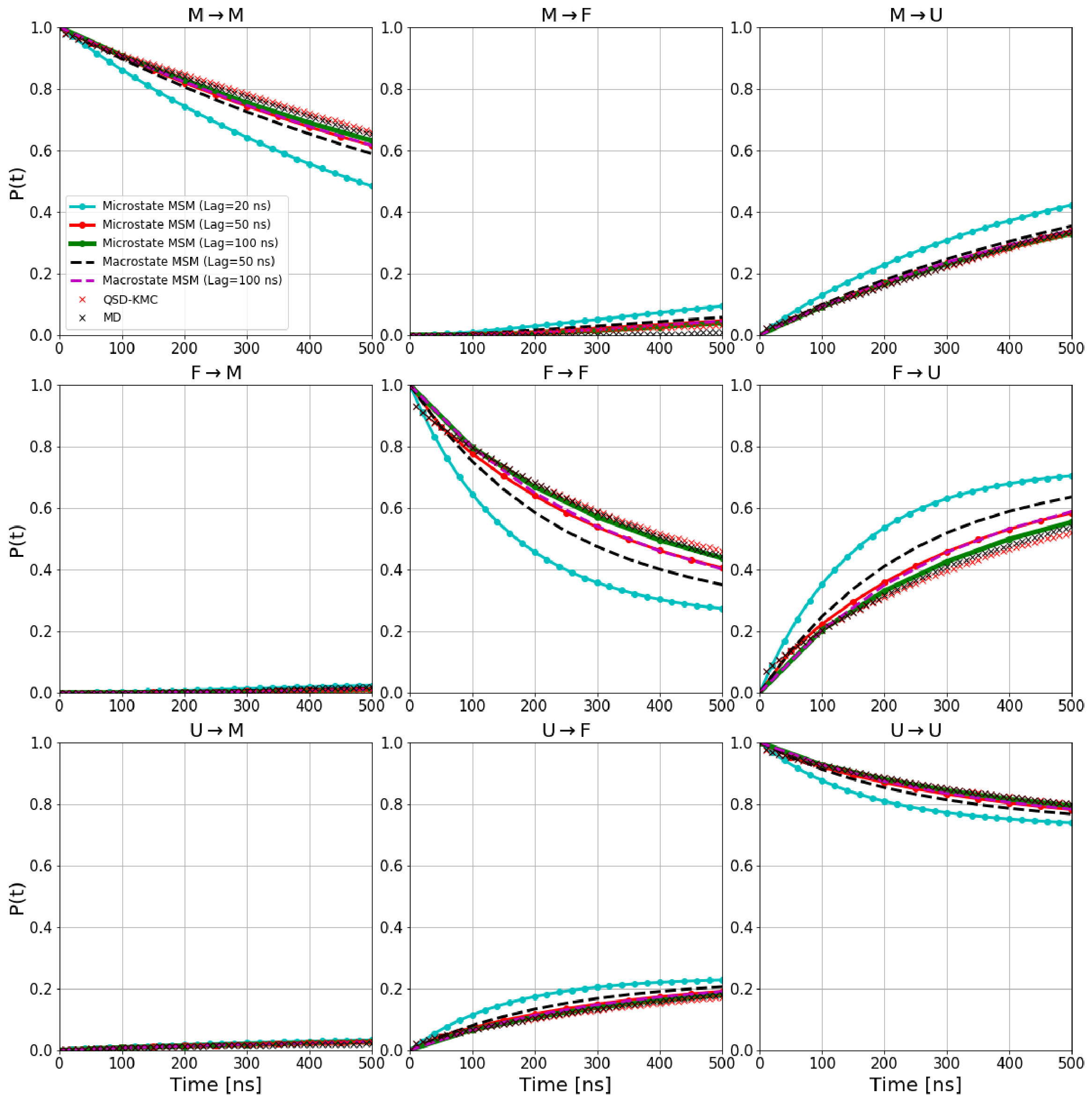 Figure 5
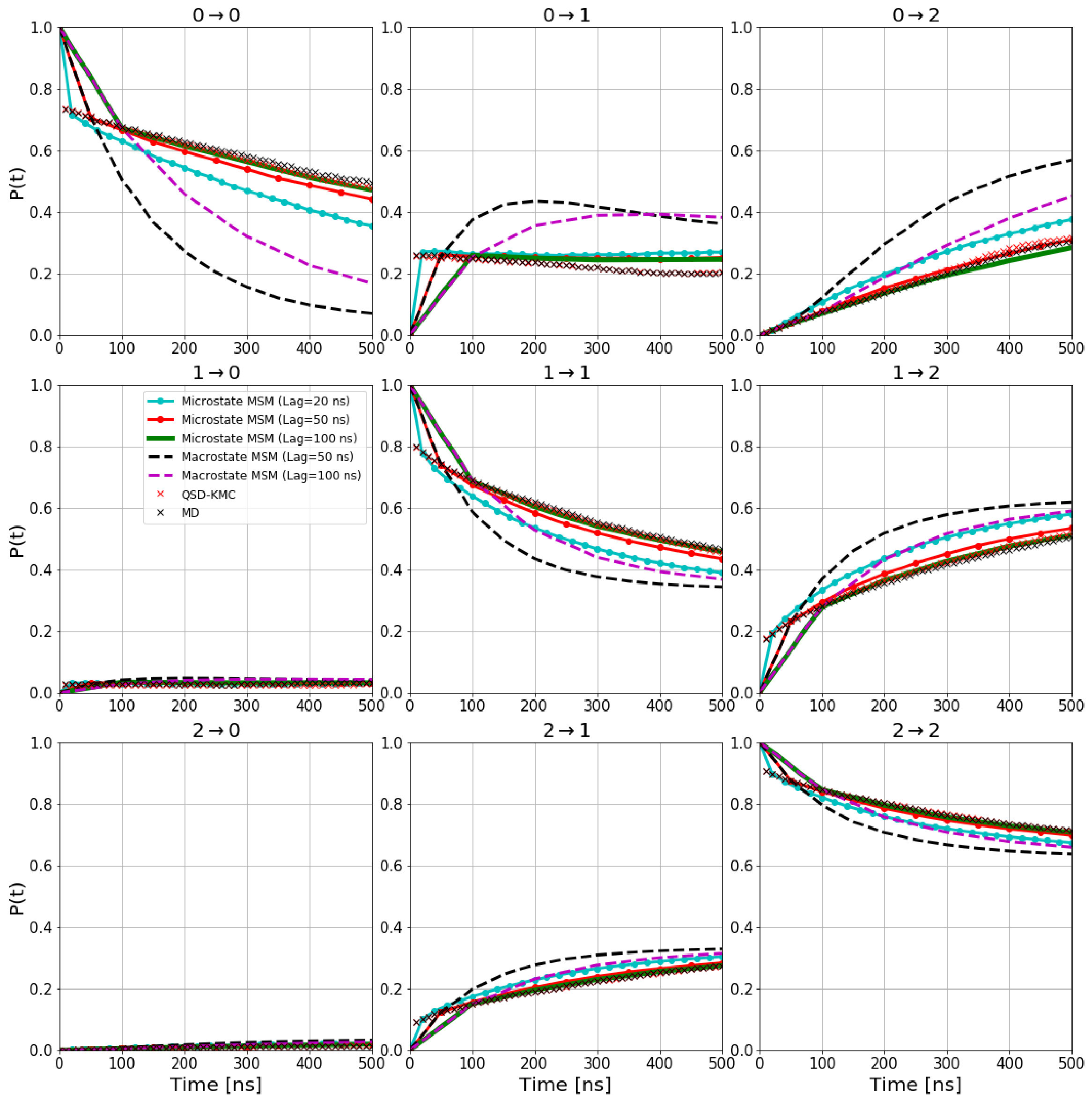 Figure 6
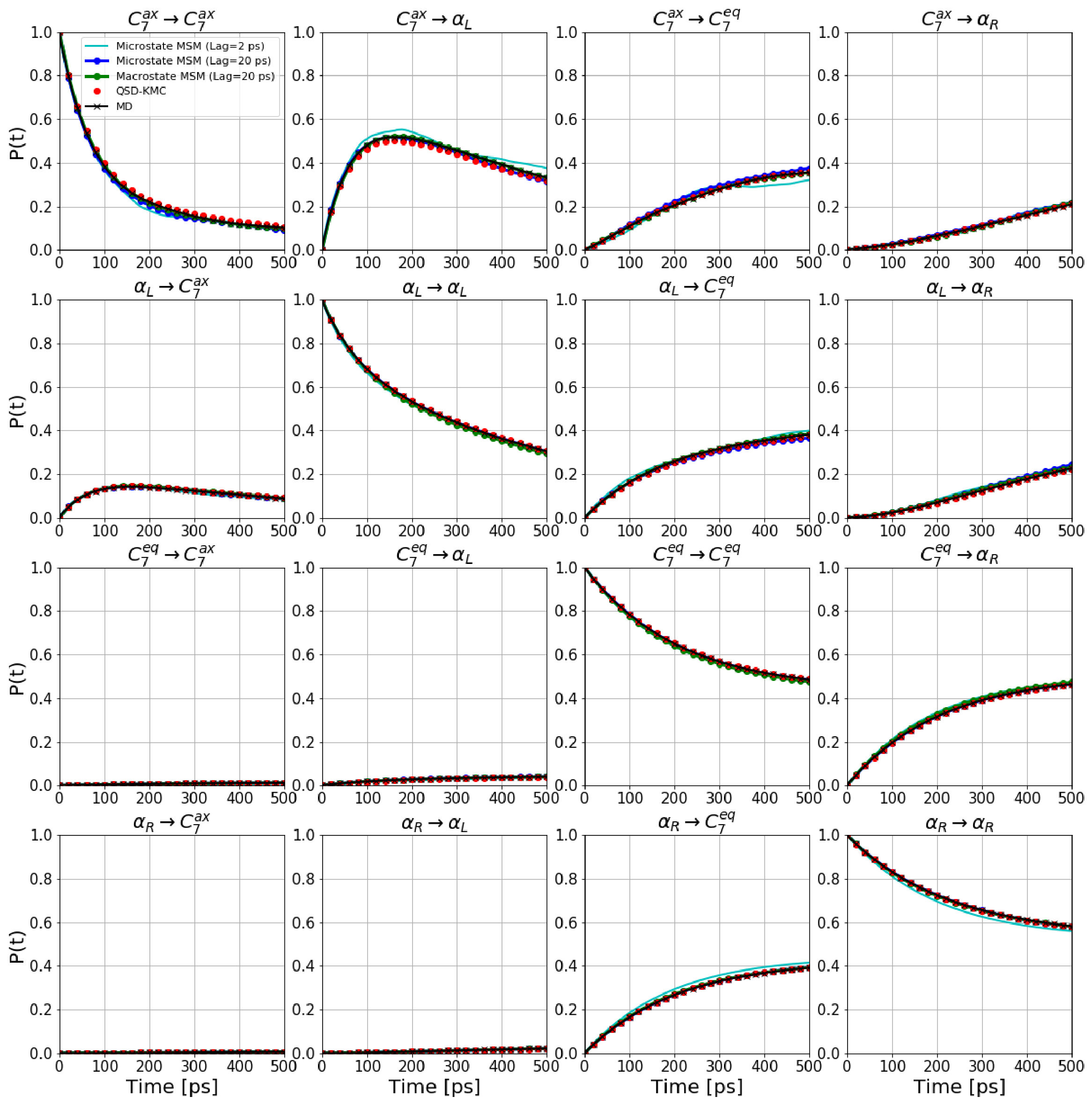 Figure 7
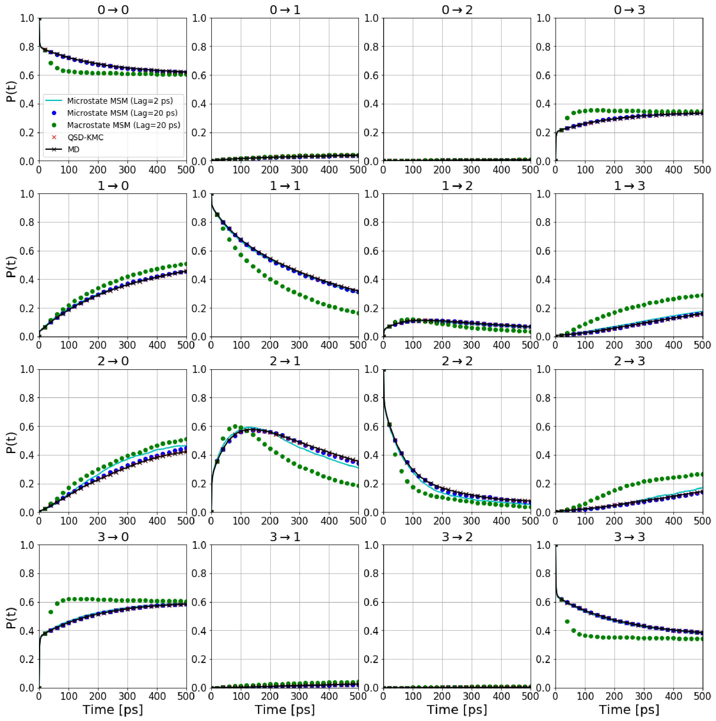 Figure 8
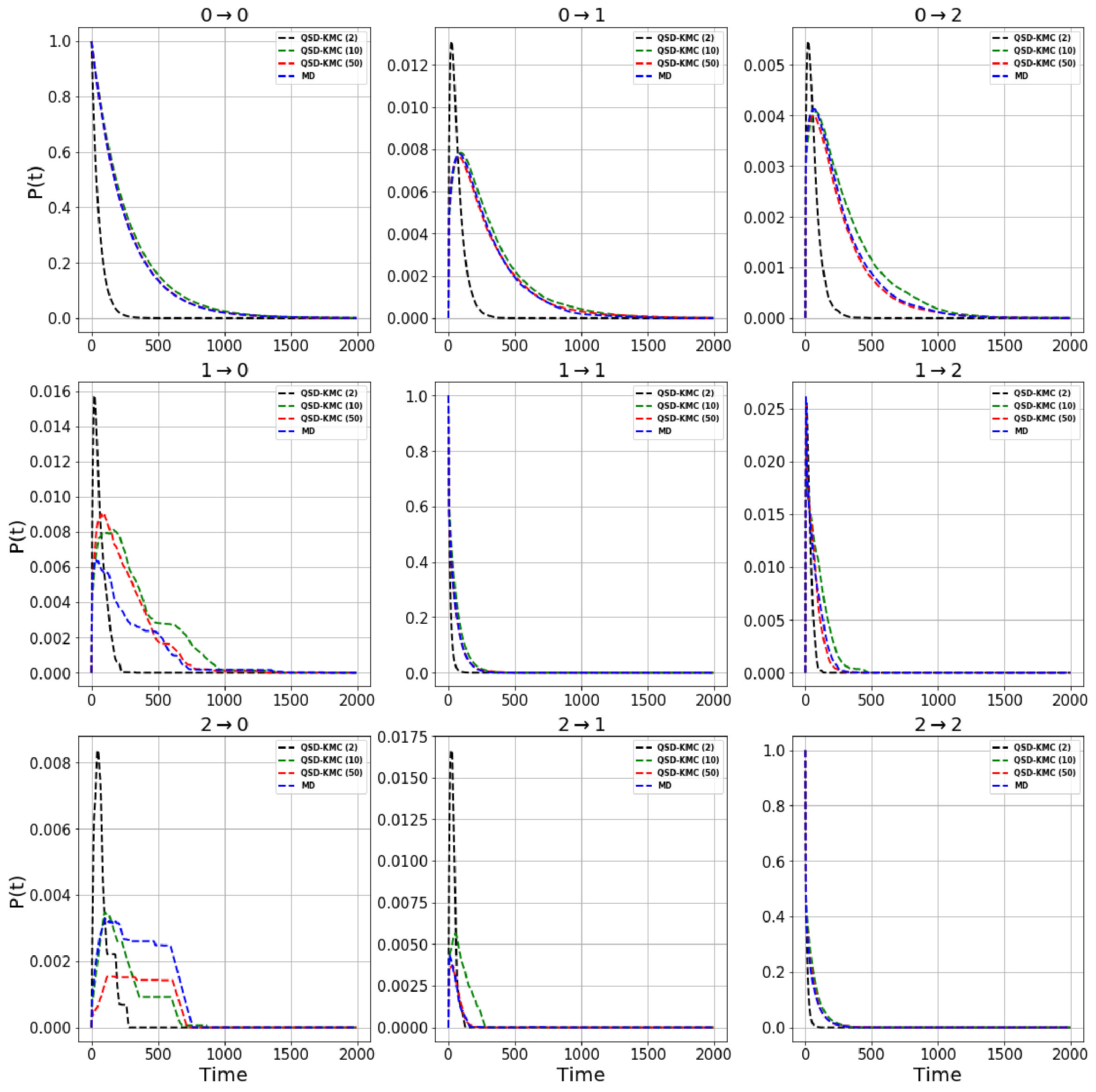 Figure 9
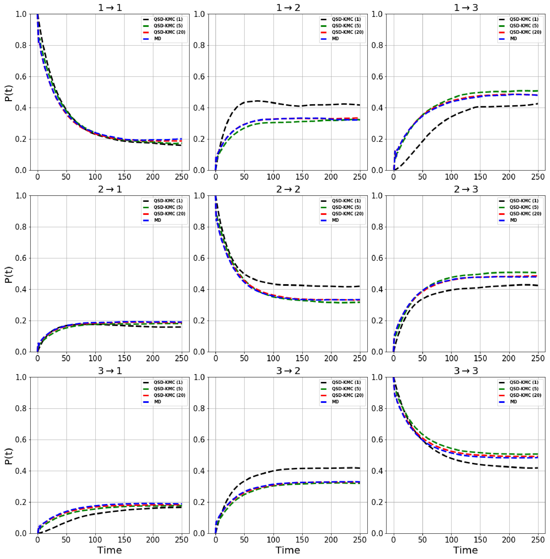 Figure 10
 Figure 11
 Figure 12
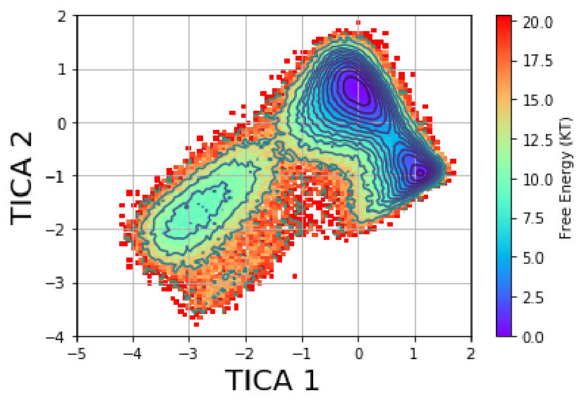 Figure 13
 Figure 14
 Figure 15
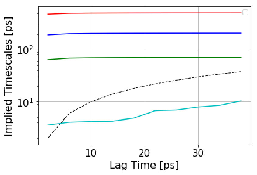 Figure 16
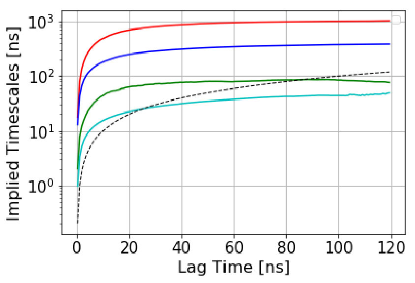 Figure 17
 Figure 18
 Figure 19
 Figure 20
 Figure 21
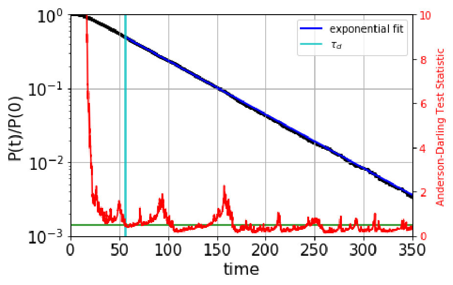 Figure 22
 Figure 23
 Figure 24
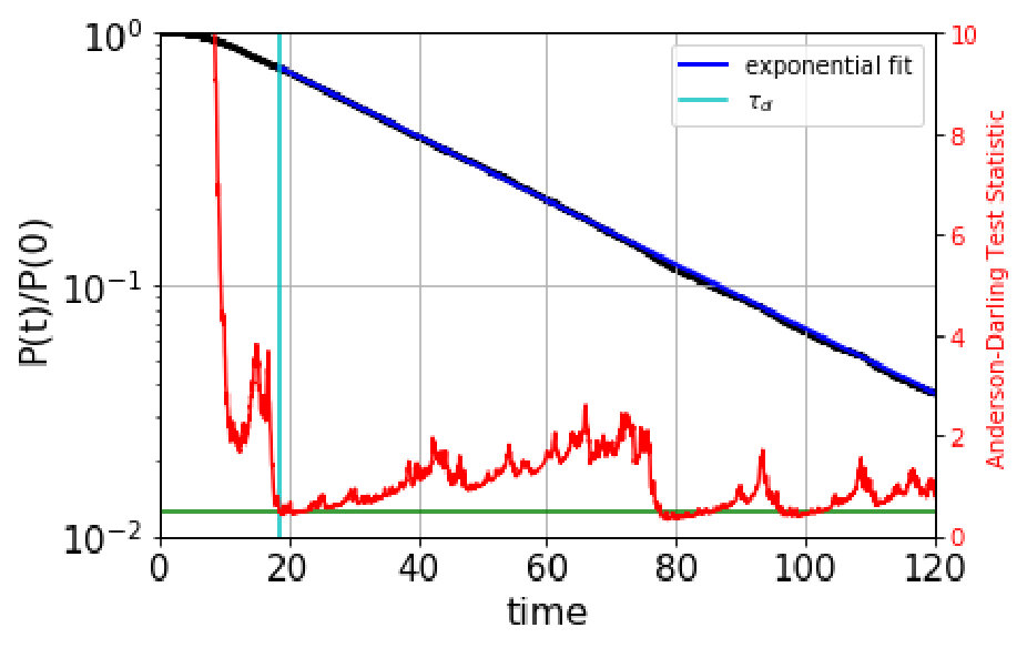 Figure 25
 Figure 26
 Figure 27
 Figure 28
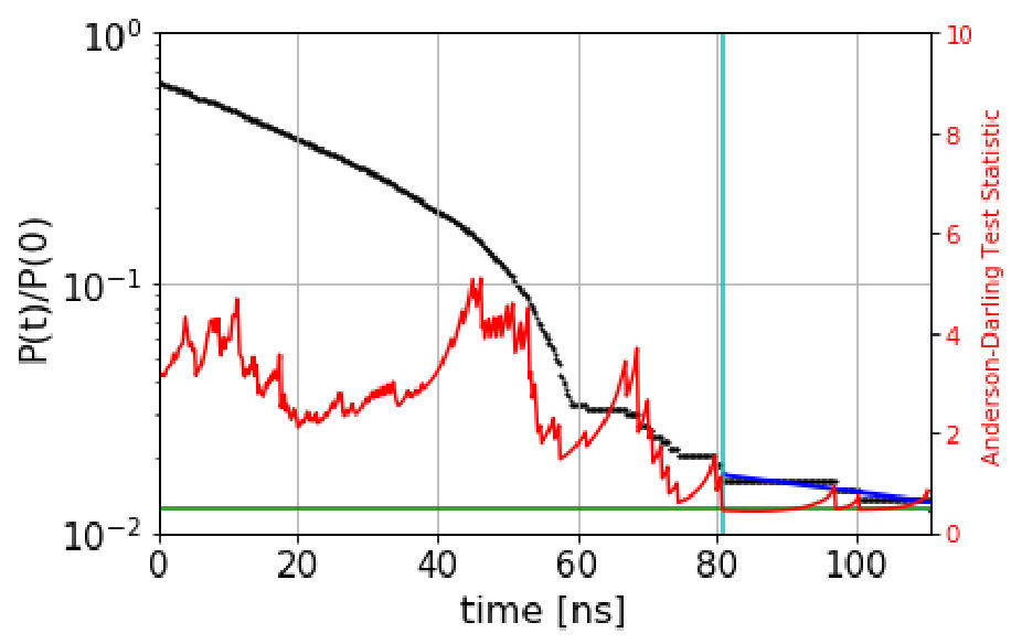 Figure 29
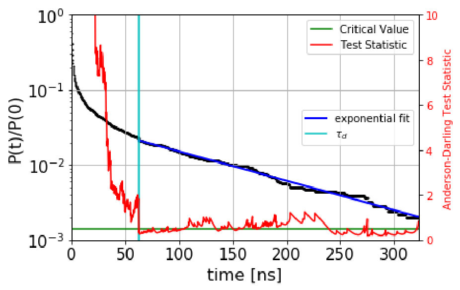 Figure 30
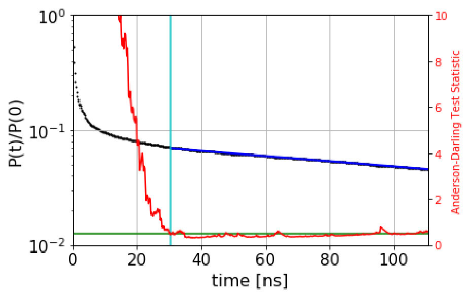 Figure 31
Peer Reviews
No public reviews on file for this paper yet. If you reviewed it on a platform where reviews are public (OpenReview, ICLR, NeurIPS, ICML), you can paste yours below so the community can read it here.
Videos
No videos yet. Explain this paper in a talk, walkthrough, or lecture? Add one.
Computing Long Timescale Biomolecular Dynamics using Quasi-Stationary Distribution Kinetic Monte Carlo (QSD-KMC)
Animesh Agarwal
Nicolas W. Hengartner
S. Gnanakaran
Theoretical Biology and Biophysics group, Los Alamos National Laboratory, New Mexico 87544, United States
Arthur F. Voter
Theoretical Division T-1, Los Alamos National Laboratory, New Mexico 87544, United States
Abstract
It is a challenge to obtain an accurate model of the state-to-state dynamics of a complex biological system from molecular dynamics (MD) simulations. In recent years, Markov State Models have gained immense popularity for computing state-to-state dynamics from a pool of short MD simulations. However, the assumption that the underlying dynamics on the reduced space is Markovian induces a systematic bias in the model, especially in biomolecular systems with complicated energy landscapes. To address this problem, we have devised a new approach we call quasi-stationary distribution kinetic Monte Carlo (QSD-KMC) that gives accurate long time state-to-state evolution while retaining the entire time resolution even when the dynamics is highly non-Markovian. The proposed method is a kinetic Monte Carlo approach that takes advantage of two concepts: (i) the quasi-stationary distribution, the distribution that results when a trajectory remains in one state for a long time (the dephasing time), such that the next escape is Markovian, and (ii) dynamical corrections theory, which properly accounts for the correlated events that occur as a trajectory passes from state to state before it settles again. In practice, this is achieved by specifying, for each escape, the intermediate states and the final state that has resulted from the escape. Implementation of QSD-KMC imposes stricter requirements on the lengths of the trajectories than in a Markov State Model approach, as the trajectories must be long enough to dephase. However, the QSD-KMC model produces state-to-state trajectories that are statistically indistinguishable from an MD trajectory mapped onto the discrete set of states, for an arbitrary choice of state decomposition. Furthermore, the aforementioned concepts can be used to construct a Monte Carlo approach to optimize the state boundaries regardless of the initial choice of states. We demonstrate the QSD-KMC method on two one-dimensional model systems, one of which is a driven nonequilibrium system, and on two well-characterized biomolecular systems.
I Introduction
Molecular dynamics (MD) is a powerful tool for probing complex processes in biological systems, such as protein folding folding1 ; folding2 , protein-ligand binding ligand1 ; ligand2 , and large scale conformational changes that lead to cellular processes cell1 . However, directly accessing the time scales relevant for such biological processes with MD is challenging, as these processes typically occur on long time scales. While the advent of specialized hardware for biological systems such as ANTON anton allows extension of the simulation time to millisecond timescales, such resources are not routinely available to researchers. This situation has motivated the development of models that can utilize information from a number of short MD simulations, which can be generated in parallel (e.g., using folding@home home1 ; home2 ), to say something about the characteristics of the longer timescale evolution. These models take advantage of the fact that these systems typically spend a period of time in a single “state” of the system, occasionally making a transition to a new state. In particular, Markov state models (MSM’s) msm1 ; msm2 ; msm3 ; msm4 ; msmvalid , which have become popular over the past decade, offer this type of approach. In MSM’s, the full configurational space is mapped onto a reduced space which is discretized into discrete states (“microstates”) and the long-time kinetics is modeled via an transition matrix where an element of this matrix represents the probability of being in state at time (the “lag time”) given that the system was in state at time . From this transition matrix one can get information on the long timescale dynamics of the system. However, the assumption that the underlying dynamics on the reduced space is Markovian induces a systematic bias in the model msmvalid .
This error in MSM due to non-Markovian behavior can be reduced either by (1) making the spatial discretization finer, which depends on the choice of the input coordinates and clustering method used or (2) decreasing the time resolution of the model by increasing the lag time, although this may prohibit investigation of faster processes that are relevant to the problem. Thus, if the state space is not optimal or the transition probabilities are calculated using a short lag time, the MSM’s may give incorrect results. Recently, aiming at this issue, Zuckermann and co-workers formulated non-Markovian estimators zuc1 ; zuc2 , which give a more accurate description of the dynamics compared to MSM’s. This analysis is based on the inclusion of a “history,” which is available in every MD trajectory. The method does not rely on the fine details of the states used and works well even if a fine time resolution is used.
Another class of methods, which has been mostly used for studying material science systems kmcmat1 ; kmcmat2 ; kmcmat3 ; kmcmat4 , is the kinetic Monte Carlo (KMC) kmc1 approach, which builds on the fact that for most material systems the dynamical evolution consists of stochastic jumps from one metastable state to another, where the system stays in a state for a sufficiently long-time to lose its memory before making a transition to the next state. Thus, if the underlying dynamics is Markovian, this characteristic can be exploited to evolve the system from one state to another over long times. However, in biological systems the energy landscapes are comprised of highly populated metastable states connected via lightly populated intermediate states, which gives rise to multiple fast processes and correlated events (such as recrossings at the dividing surface between the states); in such scenarios the underlying dynamics does not exhibit ideal Markovian behavior.
In this work we propose a new approach, quasi-stationary distribution KMC (QSD-KMC), that gives accurate long-time statistics without compromising the time resolution of the system even when the evolution of the system is complex in the way the trajectory jumps from one state to another, such that the system cannot be assumed to be Markovian. There are two key components in this KMC-based approach: (1) Calculation of the total escape rate out of a state; this is accomplished using the quasi-stationary distribution (QSD) concept (qsd1 ; qsd2 ; qsd3 ; qsd4 ), which allows direct computation of a unique value for this rate once the correlation time, or dephasing time, is known. (2) Treatment of correlated events; the effect of correlated events is included by specifying, for each KMC escape, the intermediate states and final state resulting from the escape.
With these two components, the QSD-KMC method produces, from a compact representation, state-to-state trajectories that are statistically indistinguishable from the underlying MD trajectories, for any choice of state decomposition. Moreover, we believe that the qualitative interpretation afforded by this approach, in the form of QSD escape rates and an understanding of the correlated events, is valuable even in situations where it is feasible to generate a single long MD trajectory. The concepts in the QSD-KMC approach can also be used to design a Monte Carlo method for optimization of the state boundaries. Searching for state boundaries that minimize the total correlated-event time leads to states that are, in some sense, maximally metastable. We note here that the enforcement of QSD based state-to-state dynamics adds some contraints on the length of the trajectories that we use to construct the QSD-KMC model, unlike the case with the MSM trajectories. To demonstrate the robustness of the QSD-KMC approach, we apply the method to two one-dimensional model systems, one equilibrium and one a nonequilibrium driven system, and to two different biomolecular systems with varying conformational characteristics: dialanine and villin headpiece. For the biomolecular systems, we first use state boundaries obtained via Perron Cluster-Cluster Analysis (PCCA) pccaschuette of the dominant eigenvectors obtained via diagonalization of the MSM transition matrix; for these states, we demonstrate that the state-to-state evolution characteristics from QSD-KMC match those of the underlying MD trajectories. We then demonstrate that minimizing the total correlated-event time provides a viable approach for generating good state definitions, even starting from a simple, unphysical rectangular lumping of microstates into contiguous macrostates.
The paper is organized as follows: we begin Section II with a brief overview of the QSD-KMC approach. We then discuss the standard KMC approach, the quasi-stationary distribution, dynamical corrections theory in the context of both transition state theory and the QSD, the logical connection between QSD-KMC and parallel trajectory splicing (an accelerated molecular dynamics method), and the bootstrap interpretation of QSD-KMC. In Section III, we describe the technical aspects of the QSD-KMC method, such as calculation of rate constants, the estimation of dephasing time, the procedure for generating short trajectories for constructing the QSD-KMC model, and finally lay out the algorithmic details. In Section IV, we discuss how minimizing the correlated-event time can be employed to optimize the state boundaries. In Section V, we briefly describe the procedure for comparing the results from MSMs and QSD-KMC. Finally, in Section VI, we first demonstrate the important concepts of QSD-KMC on two one-dimensional test systems and then show the robustness of QSD-KMC in applications to the two biomolecular systems.
II Theory
In this section, after a brief overview of the QSD-KMC method, we develop its theoretical underpinnings.
II.1 Brief Overview of the QSD-KMC method
The overall goal of the QSD-KMC method is to provide an accurate, compact model of the state-to-state dynamics of a complex biological system. The accuracy should be maintained regardless of whether the states are defined in a way that gives naturally Markovian behavior, or whether such a definition can even be found. The model, which is built from the information contained in a set of short molecular dynamics trajectories that probe the states of the system, consists of two main parts: 1) a set of first-order rate constants that are used in a KMC procedure to generate the next escape from the current state of the system, and 2) a set of representative instantiations for the states the system passes through, and the state it settles into, after each kinetic Monte Carlo escape. Executing the model thus involves repeating a two-step cycle, first picking a KMC escape time for exiting the current state, and then picking a particular instantiation of the state-to-state path that the model trajectory follows until it settles in some state.
As will be described in detail below, the first step in the construction of the model is to find all MD trajectory segments that spend a certain length of time, the dephasing time (), in a single state. After a trajectory has spent this much time in one state, it has lost its memory of how it entered the state and is henceforth sampling from a steady-state distribution for that state known as the quasi-stationary distribution. This distribution has the characteristics that escape from it is a first-order process, and that when an escape occurs, the boundary hitting point is independent of the boundary hitting time. For each state, following these dephased trajectory segments forward in time and measuring the number that escape per time thus gives the first-order (Markovian) rate constant for escape from the state; this rate is used in the KMC step. The second step in the construction of the model involves following each of these MD trajectories further forward in time to find the state that it settles into (spends a dephasing time in). The states each of these trajectories passes through on the way to the state it settles in, and the time it spends in each of these transient states, are stored as part of the model.
With this approach, we can take any definition of the states (though some choices would be inefficient), and obtain a compact model of the state-to-state kinetics whose accuracy is limited only by the completeness of the set of trajectories. If the states give fully Markovian dynamics, then the model will be very compact; for states, it will consist of just escape rates and final-state probabilities for each of these. When the dynamics on the set of states is not Markovian (as is almost always the case), then the model will be less compact, by roughly the minimum amount that it needs to be less compact. For each state, instead of final-state probabilities, there will be some number of representative instance trajectories giving the state-to-state path the system follows on the way to settling into a final state. We note that, if desired, the information stored for each instance trajectory can be more detailed; for example, as we will show for the one-dimensional model systems, we can model the time dependence of the trajectory position with arbitrary accuracy. Similarly, for a biomolecular system, one could choose to track the evolution through the microstates in addition to the macrostates. (We note, however, that it is typically not desirable to use microstates as the main state definitions, because the dephasing time to reach the QSD could be extremely long.) For systems with very infrequent events, such a model will still be compact, as most of the time is spent in the QSD, which can be represented with little storage.
II.2 Kinetic Monte Carlo (KMC)
A molecular system with rare-event dynamics is characterized by occasional jumps from one metastable state to another. In MD simulation of materials, it is often the case that events are rare enough so that the escape times out of a state are exponentially distributed; the transition probability of escaping a state does not depend on the history prior to entering the state, resulting in a process that is Markovian to a very good approximation. For such systems, one can circumvent the time-scale problem in MD by devising a stochastic procedure that evolves the system from state to state, since the transition depends only on pairwise transition rates for moving from state to state . If the KMC model is parameterized with accurate rate constants (e.g., from transition-state-theory calculations voterprb ), the state-to-state trajectory thus generated accurately mimics an MD trajectory projected onto the metastable states. An important property of a Markov chain is that it gives rise to a first-order process that decays exponentially; i.e. the probability that the system has not yet left state is given by
[TABLE]
where is the total escape rate out of state . The probability distribution function of the first escape time is given by
[TABLE]
Moreover, the exponential distribution holds for each pathway,
[TABLE]
We lay out the details of the KMC algorithm in Section III.
II.3 Quasi-stationary distribution
As stated above, most biological systems do not behave in a simple Markovian manner. A trajectory may leave a state shortly after entering it, in a direction that is dependent on the way it entered the state. In principle, state definitions could be designed to minimize this non-Markovian behavior, but there is no guarantee that perfectly Markovian states can be constructed. The quasi-stationary distribution (QSD) concept is the key to solving this problem. The QSD converts the escape behavior, for any state definition, to one that is Markovian, so that a KMC-like procedure can be employed. The importance of the QSD concept for rare-event dynamics was developed by Le Bris et al qsd1 in a mathematical analysis of parallel-replica dynamics (ParRep), a method for parallelizing time in molecular dynamics parrep1 ; parrep2 . Recently, the QSD-based approach to ParRep has been applied successfully to a biochemical system, attaining a parallel speedup of more than 100-fold compared to direct MD lelievrebio . The QSD also plays a key role in the parallel trajectory splicing method, which we discuss below. Here we lay out the mathematics and concepts related to the QSD. For complete mathematical proofs and details, readers may refer to qsd1 - qsd4 .
We consider the scenario of overdamped Langevin dynamics evolving on a continuous potential. In general, the arguments presented here should also apply to Langevin dynamics and many other types of dynamics qsd1 ; lelievrebio The equation of motion is given by:
[TABLE]
where the friction coefficients and the masses have been set to unity, is a point in configurational space and is the stationary Gaussian process with zero mean and unit variance. The phase space is divided into discrete states and it is assumed that the union of all the states covers the entire phase space. Consider a trajectory initiated at at a point located in state . If the trajectory has not yet escaped this state at a later time , the final configurations have a distribution given by
[TABLE]
where follows the Smoluchowski equation with absorbing boundary conditions:
[TABLE]
where
[TABLE]
can further be written in terms of the eigenvalues () and eigenfunctions () of the linear positively defined operator
[TABLE]
where are constants such that , i.e.,
[TABLE]
where is the Boltzmann distribution.
At long time, the relative contributions from the larger eigenvalues decay away, leading to the approximation for long times
[TABLE]
provided the spectral gap . The distribution continues to decay in amplitude, but it takes on a constant shape given by . The suitably normalized eigenfunction is hence referred to as the quasi-stationary distribution, or QSD. Thus, given a set of trajectories that are initiated in state , the subset of the trajectories that stay in state for a long time before moving into the next state, such that they have lost knowledge of how they got into state , give a distribution of configurations that is sampled from the QSD. It has been shown in qsd1 that once this QSD has been established, the first-escape dynamics is Markovian; i.e., escape times are exponentially distributed and the hitting point on the state boundary is independent of the escape time. To estimate the time needed to achieve the QSD to good accuracy, we note that the slowest relaxation process corresponds to the decay of the 2nd eigenvector, so we expect the dephasing to be well achieved by a time , as discussed in Ref qsd1 . We will refer to a time at which the system has come very close to the QSD as the dephasing time, .
The dephasing time is in general state-specific, so we will refer to the dephasing time for state as . We will refer to the QSD escape rate from state , i.e., the expected rate at which trajectories escape from state , conditioned on these trajectories having been in that state for at least a time , as .
II.4 Dynamical corrections
As we discussed just above, a trajectory that has stayed in a state for longer than will make its subsequent escape in a Markovian fashion, but the fate of the trajectory after this escape will not in general be a simple transition to the adjacent state with loss of memory in that state. For a complex biological system, the trajectory may enter and then exit other states in a correlated way and with complex dependencies on its past history. In this section, we discuss how this behavior is properly accounted for in our QSD-KMC method. We begin with a brief review of dynamical corrections to transition state theory; this represents the deep-state Markovian limit, leading to a formally defined rate constant between any two states of the system. We then consider the non-Markovian case, for which the QSD offers a way to recover Markovian behavior; dynamical corrections can again be applied, this time to the QSD escape rate. However, in the case of dynamical corrections to the QSD rate, the resulting state-to-state rate constants are no longer unique; they depend on the value of the dephasing time, even for long dephasing times. Nonetheless, when the dephasing times, the QSD rates, and the state-to-state rates are employed in the QSD-KMC procedure, the resulting state-to-state evolution is correct. Thus, QSD plus dynamical corrections offers a way to generalize TST plus dynamical corrections for non-Markovian systems, but the kinetic evolution of the system can only be predicted when this is done in the context of the QSD-KMC approach. We finish this section with a discussion of the relationship of QSD-KMC to the recently developed parallel trajectory splicing method, and we also present a bootstrap interpretation of QSD-KMC.
II.4.1 Dynamical corrections to transition state theory
For any system, once state boundaries have been defined, we can define the transition state theory (TST) rate of escape from each state. The TST rate () from state to state is the equilibrium flux through a dividing surface separating states and . More specifically, if one counts the number of forward crossings at the dividing surface per unit time and divides this quantity by the average number of trajectories that are in state at any time, one obtains the TST rate, . The total TST escape rate out of a state is given by
[TABLE]
where is the number of escape pathways from state . If there is a separation of time scales in the system, i.e., if the time to lose memory in some state is much shorter than the average time to escape from state , then there exists a proper first-order rate constant, , for escape from state , and the TST rate approximates this rate constant. The exact rate constant can differ from because while TST assumes that every outgoing crossing of the state boundary represents an overall reactive escape event, in reality, some of these outgoing crossings may be correlated with prior or subsequent boundary crossings. These correlated events can be in the form of recrossings, in which the trajectory quickly reenters state , or they may be “double jump”-type events in which the trajectory, while activated, quickly passes through one or more states before it finally settles into some state , losing its memory there. The number and nature of these correlated events depends on the characteristics of the system, the temperature, and the Langevin friction coefficient (higher friction increases the number of recrossings kramers and decreases the double jump probability fer1 ; fer2 ; fer3 ; fer4 ).
Assuming still that there is a separation of time scales, i.e., that the duration of these correlated events, , is much shorter than the average time until the next escape out of any state ( or ), it is possible to account, in a rigorous way, for the effect of these correlated events on the rate constants in the system chandler ; doll . The classically exact rate constant between any two states of the system, adjacent or not doll , can be written as
[TABLE]
where is a final-state-specific dynamical correction factor, which can be computed from the results of properly sampled half-trajectories initiated at the boundary to state doll . Half-trajectories that are in state at time contribute positively to if they were exiting state at and contribute negatively if they were entering state at . Specifically,
[TABLE]
where is the number of sampled half-trajectories, indicates the phase of half-trajectory (+1 if exiting state , -1 if entering state , at ), and is the Heaviside function for presence in state at time t (Note that in Ref. doll , a factor of was inadvertently omitted from the RHS of the analagous Eq. (4.6)). Thus, with TST as a starting point, and assuming a separation of time scales, this many-state dynamical corrections formalism provides a definition for the classically exact rate constants between all pairs of states in the system. Once these rates are known, a KMC procedure can be used to advance the system from state to state voterprb .
II.4.2 Dynamical corrections in QSD-KMC
In the QSD-KMC method we are presenting here, we take an approach analogous to the dynamical corrections to TST described just above, but with a key difference: we are interested in systems for which we cannot assume that we have a clean separation of time scales, i.e., systems that may not be Markovian. For such a system, although the TST rate of escape from any state () is still well defined as the equilibrium escape flux, and could be calculated if desired, it is no longer a meaningful escape rate. If the escape behavior is not Markovian, there is no simple first-order rate constant. This is where the QSD concept comes into play. For the base escape rate from state , instead of using , we use , as defined in Section II.3; this gives a good first-order rate constant for escape from state , but only after the system has spent a time of at least in that state. Then, in analogy with the use of half-trajectories to correct TST for the effect of correlated events, we follow trajectories escaping from the QSD until they settle in some state . The requirement for settling in a state is that the trajectory spends a time in that state. We note that it is possible that the correlated event may bring the system back to state , so that . While in dynamical corrections to TST, this type of return event merely contributes to a lowered overall rate of escape, in the QSD-KMC algorithm this type of returning trajectory is a meaningful event, which we track through the various intermediate states the trajectory visits before returning to state .
We will refer to these dynamical correction trajectories for QSD-KMC as instance trajectories, or instances. When the system escapes from the QSD of some state, it has a probability of settling in a certain final state, as well as probabilities for the various paths through intermediate states along the way. The instance trajectories, harvested as internal segments of the underlying MD trajectories from which the QSD-KMC model is built, give us different possible instantiations for this process. The number of instances that take the system from state to state , divided by the total number of instance trajectories for state , gives the probability that an escape from state leads to state . We note that while the QSD rate constants {} are independent of the choices for the dephasing times (provided they are chosen to be large enough), the instance trajectory sets, and their associated rate constants, are not. This is an important point that will be discussed in Section III.2.
II.4.3 Connection to parallel trajectory splicing
We note that this QSD-KMC approach makes a connection to the recently developed parallel trajectory splicing (ParSplice) method parsplice . ParSplice is a generalization of parallel replica dynamics; both methods parallelize time to accelerate molecular dynamics of rare events without requiring prior knowledge of the possible events. These methods are usually applied to material systems for which each potential basin of attraction defines a state, and the total number of states the system may visit as it proceeds is typically huge. In ParSplice, multiple trajectory segments are simultaneously propagated in one or more known states of the system; these segments are harvested and spliced end to end to make a trajectory that reaches long times. To be a valid, spliceable segment of time length , the trajectory must have remained in a single state for a time prior to the beginning of the segment, and also must remain in a single state (the same or another) for the final of the segment. Spliceable segments thus fall into two classes: those that remain in one state the whole time (very common for a rare-event system) and those that make one or more transitions during the segment. We see then that transitioning segments in ParSplice are exactly the same as the instance trajectories defined for QSD-KMC.
II.4.4 Bootstrap Interpretation
Any trajectory can be segmented into excursions each time a dephasing event occurs. The loss of memory of the past after a dephasing event implies that the excursions are independent and identically distributed conditionally on the state in which the dephasing event occurred. Given an ensemble of excursions, we can construct a bootstrap path by resampling the excursion from the appropriate subset (given the initial state). This interpretation shows that the statistical accuracy will depend on the number of excursions starting in each state.
III Algorithm and Practical Aspects of Implementation
In this section, we describe the practical aspects of implementing the QSD-KMC method. We first discuss the Anderson-Darling test procedure that we use for estimating the dephasing time. Next, we discuss how the pairwise rate constants are calculated in this model. We then lay out the procedure for generating the short trajectories for constructing the QSD-KMC model. Finally, we discuss the QSD-KMC algorithm in detail and how it can be applied in practice to generate exact state-to-state evolution in a biological system.
III.1 Choice of dephasing time
Choosing an appropriate dephasing time is a key part of the QSD-KMC algorithm. For very-low-dimensional systems, it is possible to directly calculate a good estimate of the dephasing time by appealing to the expression for the error in the QSD derived by Le Bris et al. qsd1 , , where and are the first two eigenvalues of the Fokker-Planck equation with absorbing boundary conditions, as discussed above. For higher-dimensional systems, where it becomes unfeasible to solve the Fokker-Planck equation, direct calculation of is extremely difficult. For the purpose of demonstrating the QSD-KMC method, we estimate for each state as the point in time when the survival probability becomes exponential. We note that, as pointed out by Le Bris et al qsd1 , this does not guarantee the system has achieved the QSD. However, we believe this approach will suffice for our purposes here. Indeed, in the results section below, we will find that using this approach we obtain very accurate results. The QSD-KMC trajectory predictions agree extremely well with the results calculated from the underlying MD trajectories. For systems with very deep states, it is no longer feasible to use the onset of exponentiality to define the dephasing time, as it requires running each trajectory long enough to see an escape. In this situation, we suggest using the Gelman-Rubin approach gelman as proposed by Binder et al qsd2 and recently implemented by Hedin and Lelievre lelievrebio .
We automate the determination of the onset of exponentiality by employing the Anderson-Darling test anderson for an exponential distribution. Normally, the Anderson-Darling test is used to rule out, to high confidence, that data comes from a given distribution, by comparing a test statistic, computed from the data, to a critical value that depends on the desired confidence; if the test statistic is greater than the critical value, then the null hypothesis (that the data is exponential) is rejected. (For example, =1.3 for 95% confidence, or a value of 0.05.) Here we use the Anderson-Darling test in the opposite sense, seeking reassurance that the data is not too likely to violate exponentiality. We achieve this by requiring that the standard test statistic anderson be below a much lower critical value of . We determined this critical value empirically: data drawn randomly from a true exponential gives a test statistic that is below =0.5 roughly 50% of the time. For computing the test statistic, we use the standard scipy.stats library in python.
The automated procedure then works as follows. We scan candidate values of the dephasing time, , computing the Anderson-Darling test statistic for the escape-time data with escape times less than discarded. The dephasing time is then set to the lowest value of for which the test statistic is less than 0.5. As an example, Figure 1 shows the survival probability function and the Anderson-Darling-determined dephasing times for the three states of villin headpiece. (These states were obtained via the application of MSM and Perron Cluster-Cluster Analysis (PCCA) pccaweber ; the free energy map of villin headpiece and the three states are shown in the figures in Section VI. More details on how we characterize these states as misfolded, folded and unfolded are also given in Section VI.) We observe that the Anderson-Darling test procedure is quite sensitive to the nonexponentiality, and appears to give a fairly conservative determination of , a desirable characteristic.
III.2 Calculation of rate constants
Once the dephasing time for a state has been estimated, the first-order escape rate out of the QSD for that state, , is given by the negative slope of the log of the survival probability for times greater than . Alternatively, one can calculate this rate as the average escape rate for the trajectories after time , provided all these escape times are known (i.e., that no trajectories are prematurely terminated). By definition, these rates do not change (or should change very little) as the dephasing time is further increased. The QSD escape rates {}, along with the instance trajectories, are all that is needed to carry out QSD-KMC simulations. However, before leaving this section, we make a few other points about rates in this type of model.
Once first-order QSD escape rates out of a state have been estimated, the pairwise rate constants accounting for the correlated dynamical events can be defined as
[TABLE]
where is the probability that, starting in state , the trajectory first settles (resides for at least a dephasing time, as discussed above) in state . We note that is analogous to , discussed above for the case of dynamical corrections to TST in a system with a clear separation of time scales. However, there is an important difference: (and hence ) depends on the choice of dephasing times for the states, even when all the dephasing times are appropriately large. That will vary with the dephasing time can be easily understood from a simple thought experiment on a three-state system with states 1, 2, and 3. Starting with a conservative (long) value for the dephasing time for all the states, the rate constants can be calculated using Eq. 14. Focusing on , if we further increase , the probability that the system settles in state 2 will be reduced; it becomes more likely that the system fails to stay long enough in state 2 to be declared as settled, and instead makes additional transitions, ultimately settling with greater likelihood in state 1 or 3. Thus, is reduced as we increase .
We can also define pairwise rate constants () corresponding to the state first encountered upon escape from the QSD,
[TABLE]
These rates are not dependent on the dephasing times (once the dephasing times are large enough to give accurate QSDs), since the hitting point on the state boundary is independent of the escape time once the QSD is established qsd1 . Thus, although and {} are fundamental properties of the system once the state boundaries are defined, the settling rates {} are not.
To summarize, the QSD escape rates {} generated for use in the QSD-KMC model are unique once the state boundaries have been specified and suitably long dephasing times have been determined. Adjacent-state hitting probabilities (not needed for the QSD-KMC procedure) are also unique. However, for a complex biological system, the settling rates {} will in general have no unique value; they will continue to change as the dephasing times are increased. This is a natural consequence of the non-Markovian nature of these systems. The key point, though, is that in spite of this characteristic, using these settling rates in the QSD-KMC procedure will generate appropriate and accurate predictions of the state-to-state dynamics, for any (safe) choice of dephasing times.
III.3 Generating and Analyzing the Short Trajectories
Here we specify the procedure for generating the short trajectories such that they are long enough (and just long enough) to allow extraction of the information for constructing the QSD-KMC model. We assume that the user has chosen a set of reaction coordinates and defined the states in that subspace. There are two stages in the method:
Stage 1: Determining the dephasing times and QSD escape rates.
For each state :
- •
Initiate a number of trajectories.
- •
Integrate each of these trajectories forward in time until it escapes from state .
- •
Using this list of escape times, apply the Anderson-Darling procedure discussed above to determine the appropriate dephasing time . Also determine the QSD escape rate for this state.
Stage 2: Creating the instance trajectories.
For each state :
- •
Discard the trajectories initiated in state that escaped before .
- •
For each of the remaining trajectories, continue integrating the trajectory forward in time until it dephases (settles) in some state , where may be the same as . Record the desired information about the instance trajectory, from the time it left state until the time it finished dephasing in state .
We note that this procedure generates a set of trajectories with varying lengths. It is generally not sufficient to generate a set of short trajectories that are integrated for a fixed time unless the fixed time is fairly long. If any trajectories are truncated before they escape from their initial state, it becomes difficult to properly determine the QSD escape time and the dephasing time. Moreover, if any trajectories are truncated before settling into a final state, a bias will be introduced into the QSD-KMC model, because instance trajectories that are long (i.e., that visit many intermediate states) are then less likely to be included in the model.
As mentioned above, for systems with very deep states, it may not be feasible to use the onset of exponentiality to define the dephasing time, as it requires running every trajectory long enough to see an escape. In this situation, the procedure could be modified as follows:
Stage : Determining the dephasing times and escape times.
For each state :
- •
Initiate a number of trajectories.
- •
Integrate these trajectories forward in time, replacing any that escape from state using a Fleming-Viot cloning procedure fleming1 ; fleming2 .
- •
Determine when dephasing has been achieved using the Gelman-Rubin criterion (this also defines ).
- •
Continue these dephased trajectories forward in time until some number of them have escaped. The QSD escape time () can be determined by averaging these escape times, noting that each successive escape time, relative to the previous escape time, should be reduced by a factor of the number of dephased trajectories remaining in the state, to account for the parallelization speedup (as in parallel-replica dynamics parrep1 ).
Stage : Creating the instance trajectories.
For each state :
- •
For each of the trajectories that escaped after dephasing, continue integrating the trajectory forward in time until it dephases (settles) in some state , where may be the same as . Record the desired information about the instance trajectory, from the time it left state until the time it finished dephasing in state .
III.4 Algorithm
KMC algorithm: Suppose the system is in state ; there are pathways along which the system can make a transition. The probability distribution of the first escape time for each of the pathways is given by . One can draw a time from the exponential function for each of the pathways via where is a real random number between 0 and 1. This time is representative of a first escape time for a first-order process. One then finds the pathway that has the minimum value of , the system is moved to state , and the simulation clock is advanced by . The more efficient version of this algorithm involves stacking all the rate-constant objects (where each object has a length equal to ) end to end and choosing a random number between 0 and (where ). The object associated with the chosen random number is the pathway that the system follows and the simulation clock is advanced by time . This approach is referred to as the Bortz, Kalos and Lebowitz (BKL) algorithm bkl .
QSD-KMC algorithm: The idea is quite similar to the BKL algorithm described above. Suppose the system is in state . We draw an exponentially distributed time using the total escape rate : , and advance the simulation clock by this time. Next, we pick a random position along an array of trajectory instances for state . The chosen instance defines the pathway that the system follows through intermediate states and the state that it finally settles in. The simulation clock is advanced by the total time the instance trajectory spends going through all the intermediate states as well as the dephasing time of the final state into which it settles. The system is then moved to the new state and the process is repeated again with the list of pathways and rates for state . A schematic representation of the QSD-KMC procedure is shown in Figures 2(a) and 2(b).
QSD-KMC predicts the state-to-state evolution with accuracy that improves with increasing and total underlying trajectory time . Similar to the other state-of-the art methods such as MSM, the long time dynamics is predicted from a compact model built from a database of short MD simulations, although there is an additional constraint regarding the length of the individual MD trajectories that depends on the macrostates, as discussed above in Section III.3.
There are two main sources for errors in QSD-KMC. The first one is the statistical error arising from observing only a finite number of transitions from one dephased state to another, which leads to uncertanities in the estimated rate constants. One way to reduce this error is to leverage an adaptive-sampling approach adapt , wherein by observing the uncertanities in the rate constants, one can initiate additional simulations in states that have a large contribution to the uncertainity. The other source of error is the increasing uncertainty in the QSD-KMC predictions at longer times, due to the possibility of missing rates and pathways abhi1 ; abhi2 on these timescales. Following Chatterjee and coworkers abhi1 ; abhi2 , we can define the validity time of a KMC model, i.e. the time duration for which the KMC model continues to give correct dynamics compared to the underlying MD dynamics, after which the predictions are less reliable. This error can be reduced by employing some of the techniques described in abhi3 to boost the validity time of the model.
IV State Optimization
Here we propose a Metropolis Monte-Carlo method that optimizes the shapes of the macrostates, such that the states obtained correspond, in some sense, to the set of states that are maximally metastable. The procedure is based on the minimization of the total time of the correlated events in a long QSD-KMC trajectory normalized by the length of the trajectory. Consistent with the discussion above, the correlated event time begins upon escape from a state in which the trajectory spent at least a dephasing time, and ends when the trajectory has spent at least a dephasing time in some (perhaps the same) state. For a given number of macrostates (), the procedure thus identifies the partitioning of the state space into contiguous states that minimizes the total correlated event time in a given set of MD trajectories.
While the procedure we will describe can in principle be applied to any system studied with QSD-KMC, in fact it may not be so straightforward when one has pre-generated a set of short trajectories. This is because as the state definitions change during the optimization, strictly obeying the two-stage procedure described in Section III.3 dictates re-evaluating the dephasing time for each state, and this in turn may require extending the length of some trajectories to re-satisfy the requirement that every trajectory fully settles in a final state. The optimization procedure is thus coupled to the running of the trajectories. On the other hand, there may be effective ways to achieve the optimization approximately with minimal modification of the trajectories. Also, sometimes one has available very long trajectory segments, as is the case for the alanine dipeptide example below, so that multiple instance segments can be taken from a single trajectory, and each instance segment can be extended as necessary with only a very low probability of coming to the end of the trajectory. In this case only a very small bias error is introduced by the finite trajectory length. Finally, for the case in which a very long, single trajectory is available, as is the case for the villin headpiece example below, the procedure can be applied with essentially no error arising from the finite trajectory length.
The process is initiated by providing a starting guess for the definition of the states, perhaps from PCCA, or from a simple geometric partitioning, in terms of the basis of the microstates. Given this initial lumping of microstates into macrostates, we calculate the average fraction of the QSD-KMC trajectory time that is involved in correlated events. We will refer to this as the fractional “outside” time, , because the trajectory is outside of any QSD for this fraction of the time. If the MD trajectory information underpinning the QSD-KMC model is “balanced,” i.e., if the trajectories are each long enough to have visited all the states many times, or if the number of trajectories initiated in each state is proportional to the equilibrium population of that state, then can be computed directly from the state-projected MD trajectory information, without generating any QSD-KMC trajectories. In this case, is then simply given by the total instance time divided by the total MD trajectory time that was usable in generating the instance information. We exploit this approach in the present work. If the trajectory information is not balanced, then can be computed from a sample set of QSD-KMC trajectories or, alternatively, it can be computed for each state from and the average length of the instance trajectories escaping from state , and these can be weighted by the equilibrium population fractions obtained from the first eigenvector computed from diagonalization of the appropriate transition matrix.
To generate a trial move in the Monte Carlo procedure, a microstate is chosen at random, and a microstate that is a neighbor to microstate is also chosen at random. If and do not belong to different macrostates, the trial move generation is repeated until they do, which is considered as one Monte Carlo step. The macrostate assignment of is then changed to match the macrostate of , and the outside fraction is calculated for this new definition of the states. If f^{out}_{trial}$$<$$f^{out}, we accept the new partitioning, and otherwise we accept it with Metropolis probability , where denotes inverse temperature. In this work, we use a very simple simulated annealing schedule in which is equal to , where is the Monte Carlo step number. We perform 5,000 Monte Carlo steps in each application of the method and check for the convergence of . Since the method generally improves the state boundaries at each MC iteration, we determine the new dephasing times for the states using the Anderson-Darling procedure after every 200 Monte Carlo steps. This procedure gives an “on-the-fly” estimate of the dephasing times and also minimizes the correlated event time in a way that is more specific to the dephasing times. As a final step, after this Metropolis walk is converged, we restart the procedure using a very low temperature, so that essentially no uphill steps are accepted, and stop this procedure after 5000 Monte Carlo steps. Although the method should be applicable to an arbitrary partitioning of macrostates, it is advisable to initiate the process with a set of states that do not require extremely long dephasing times. For every system, we initiated 50 Monte Carlo runs starting from the same state decomposition but with a different random number seed, and we selected the partitioning with the minimum value of . We note that this framework is similar to the one developed by Chodera et.al. choderapart , where the goal was to discover the kinetic metastable states by maximizing the metastability index of a partitioning into macrostates. The metastability was defined as the sum of self-transition probabilities at a given lag time, , where is the number of macrostates and denotes the self-transition probabilities.
V Procedure for comparing MSM and QSD-KMC
In the results below for the biochemical systems, we employ states defined by the Perron Cluster-Cluster Analysis (PCCA) pccaweber and compare the QSD-KMC results to those from a Markov State Model (MSM) msm1 - msm4 . Details of the MSM and PCCA methodologies are given in the supporting information. The output of PCCA is a fuzzy clustering of microstates to macrostates. However, in this work, we always consider the crisp assignment of the microstates to the macrostates and avoid the fuzzy assignment altogether, as QSD-KMC provides dynamical evolution of states with well-defined boundaries. In the MSM framework, this is achieved by generating a synthetic “microstate” trajectory at a given lag time and mapping it onto the crisp macrostates (from here on, we will refer to this model as microstate MSM). In addition, we show the results from a Markov model where the transition probability matrix is constructed directly over the set of macrostates (this model will be referred to as macrostate MSM). This allows us to make a direct comparison of QSD-KMC macrostate evolution with the results obtained from different Markov models. For evaluating our state optimization approach, we calculate the implied timescales by analyzing the transition matrix constructed on the final set of macrostates obtained and compare them with the timescales obtained via diagonalization of the transition matrix built using the crisp PCCA states. In this work, we use the PyEMMA software package pyemma for MSM construction and analysis.
For validation of long time scale dynamics, we calculate the macrostate probability evolution, i.e., the probability to be in state at time given the system was in state at time [math], for both the QSD-KMC trajectories and the MD trajectories for all the states. The precise definition of this function is
[TABLE]
where is the number of trajectories, is the length of trajectory and is the state of the system in trajectory at time . In constructing the probability evolution plots for QSD-KMC using Eq. 16, we make no distinction between residence in a state where the trajectory remains longer than a dephasing time and transient residence in that state during a correlated-event sequence. We believe this gives a meaningful definition of the state occupancy as a function of time for the purpose of calculating this function. However, we note that because the properties of a system passing through a state quickly are not necessarily the same as the properties of a system that has settled into that state, using this state probability evolution function weighted by the equilibrium macroscopic property of each state is not sufficient to compute a fully accurate time evolution of the macrosopic properties of the system. On the other hand, as mentioned in Section II.1, greater detail about the instance trajectory can be stored if desired; e.g., the microstate as a function of time can be recorded.
VI Results and Discussion
In this section, we first discuss the core concepts of QSD-KMC method on two easily visualized systems: a one-dimensional three-well potential and a nonequilibrium system consisting of a one-dimensional sloped sine-wave potential. We show that the QSD-KMC trajectories accurately reproduce results from long benchmark MD simulations on the same systems. We then compare the dynamics obtained from QSD-KMC with the underlying MD dynamics for two different biomolecular systems, dialanine and villin headpiece, to demonstrate the practical applicability of QSD-KMC to extract long time scale dynamics and the minimization of the outside time as a state optimization method. These systems enable us to show the potential of the QSD-KMC method to generate arbitrarily accurate statistics at any time resolution in scenarios where the dynamics consists of strongly metastable (long-lived) and weakly metastable (short-lived) states, thereby giving rise to multiple slow and fast processes. Such an analysis validates the robustness of the method to generate correct long-time statistics when the dynamics does not exhibit ideal Markovian behavior. The results for these biomolecular systems are structured as follows. First we define states based on MSM and PCCA. We calculate the probability evolutions using QSD-KMC, microstate MSM (at two lag times) and macrostate MSM, and compare them to the results from the MD trajectories. Then we use simple rectangular state boundaries for the same number of states and evaluate the resulting probability evolutions using these three approaches. Finally, we apply the outside-time based state optimization method, starting from the simple rectangular state decomposition and show how well they reproduce the state boundaries obtained using PCCA.
One-dimensional potential – equilibrium system
We first consider dynamics in a one-dimensional, three-well potential. This allows us obtain results to very high precision, making the accuracy of the method very clear. The potential, shown in Figure 3(a), is a sloped cosine curve with a curvature-matched harmonic wall on the left side of the lefthand state (state 1) and on the right side of the righthand state (state 3),
[TABLE]
where is the slope. In this system, the three states are very similar other than being at different energies. We use a fairly low friction so that double-jump correlated events are more likely to occur. We integrate the Langevin equations of motion using the BAOAB method boab , using =0.5, friction = 0.1 inverse time units, time step = 0.05 and mass = 1.
The benchmark simulation providing the correct answer is a single, long MD simulation, of length 2,000,000 time units. To generate the QSD-KMC model, 10,000 short trajectories were initiated in each of the three states; each trajectory was continued until it escaped from its state. This corresponds to the first stage of the two-stage procedure described in Section III.3. We determined the dephasing time for each state using the Anderson-Darling procedure described in Section III.1, as shown in Figure 3(b) for state 2. There is clearly a significant deviation from exponentiality at times shorter than 20 time units, after which the Anderson-Darling statistic rapidly drops down to the 0.5 threshold. Applying this dephasing time, roughly 25% of trajectories were discarded from each state, and the QSD escape times were determined from the average escape times, offset by , of the remaining trajectories. Then, following the second stage of the procedure, these remaining trajectories were continued forward until they dephased again in some state, each of these representing an instance trajectory.
Figure 3(c) shows the QSD density for state 2, generated by sampling points from trajectories that have remained at least a time in the state. (The QSD densities for states 1 and 3 are very similar to this.) The QSD density, , is clearly different than the equilibrium (Boltzmann) distribution, , which was generated using a Metropolis Monte Carlo procedure, rejecting steps that attempted to leave the state (i.e., corresponding to reflecting boundary conditions). The QSD is more peaked in the center of the state, and has less density than near the boundaries. This is a general characteristic of QSDs, caused by the absorbing boundary condition at the edge of the state. Some trajectory points near the boundary that would contribute to the Boltzmann density are missing from the QSD density because near the boundary there is a higher probability that the trajectory entered the state recently, more recently than a dephasing time. For very deep states, approaches the shape of , because the potential energy is so high near the edge of the state that further depletion by the absorbing boundary is hardly noticeable.
Figure 4 shows the state-to-state probability evolution calculated from the benchmark MD trajectory and from the QSD-KMC trajectories at different dephasing times. The QSD-KMC curves (at = 20 time units) are seen to agree extremely well with the direct MD result; however for a short dephasing time, the results from QSD-KMC disagree with the MD results, signifying the importance of the dephasing time.
Because of the simplicity of this system, it was easy to store the trajectory position at every MD step along each instance path (i.e., from the instant the trajectory left its initial state until the time it finished dephasing in the final state). This is in contrast to the biochemical systems we present below, for which only the macrostate information was stored (although it would be easy to store the microstate information along the instance path as well). Using this detailed information, we have a model that can predict the evolution essentially continuously in time. For example, in Figure 3(c), we can see that the density accumulated along the path of a long QSD-KMC trajectory gives a precise match to the Boltzmann density, as it should for a system in equilibrium. To compute this QSD-KMC density, the trajectory positions along the QSD-KMC path are stored and binned into a histogram, and the histogram is normalized for each state. This QSD-KMC density is comprised of contributions from trajectories that pass through the state without settling (e.g., as part of a double jump or longer jump), as well as contributions from the QSD density for time durations when the system is in the QSD and has not yet reached the next escape time. In Figure 5 we show how the density obtained from a QSD-KMC trajectory varies with the dephasing time. It can be clearly seen that the distributions constructed using a very short dephasing time disagree with the MD results, showing that the information from the MD data is not simply reused; establishment of the QSD within the states plays a significant role in generating accurate statistics.
One-dimensional potential - nonequilibrium driven system
Next we consider driven, nonequilibrium dynamics in the one-dimensional sloped cosine-wave potential given by
[TABLE]
where is the slope. This potential is shown in Figure 6(a). The exact MD benchmark for this system is computed by initiating trajectories in state 0, the highest-energy (and a relatively deep) state. After equilibration in state 0, each trajectory escapes from this state and falls down through the staircase of wells; it loses its memory and equilibrates in some wells, but passes quickly through others. There is no end to the staircase, so equilibrium is never achieved. A trajectory may hop back up the staircase in some cases, but it is more likely to escape in the forward direction. Because we employ a very low Langevin friction, there is a high probability that it will simply pass through a state as part of a correlated multiple-jump event, and for a trajectory moving in the direction, this probability increases with the length of the jump, as it tends to pick up speed at this low friction. (Ferrando et al fer3 have directly studied the friction dependence of the jumping behavior in a tilted cosine system). This is clearly non-Markovian dynamics, and we demonstrate the accuracy of the QSD-KMC method, again implemented using many short trajectories, by comparing the predicted steady-state density in for this nonequilibrium system with the exact MD benchmark.
The integration method and parameters are the same as in the equilibrium three-state system, except that the friction is lower ( = 0.05 inverse time units). To generate the QSD-KMC model, 100,000 short trajectories were initiated in each of states 0 through 4, and 10,000 trajectories were initiated in each of states 5 through 10. The two-stage procedure to determine the dephasing times, the QSD escape times, and the instance trajectories was then carried out just as in the three-state model above, except that any trajectory that reached state 11 was terminated, on the assumption that it had a negligible chance of returning to state 2 or 1, the states we focus on in our analysis. For the long-MD benchmark results, we averaged over 100,000 trajectories that were initially equilibrated for 50 time units in state 0. The termination at state 11 was again imposed.
The Boltzmann probability density for state 1 is shown in Figure 6(c). Even though this is a nonequilibrium system, this Boltzmann density is exactly the same as for the equivalently shaped middle state (state 2) of the three-state equilibrium system. If the friction setting were the same, this would also be true of the QSD density, the Anderson-Darling behavior, and the dephasing time. However, because we are using a lower friction, the QSD density changes and the dephasing time increases to 55 time units, compared to 20 time units for the three-state system, as can be seen in Figure 6(b). As in the three-state case, we store the trajectory position at every time step along each instance trajectory segment, making it possible to generate the density accumulated along the QSD-KMC trajectory path to high precision in .
Focusing on state 1, Figure 6(c) shows that the QSD-KMC density, agrees essentially perfectly with the exact MD results. QSD-KMC is giving the correct nonequilibrium density for this system at every point in space. Because this is a nonequilibrium system, the density in state is a function of both the shape of the potential within state , as well as shapes and connectivities of the states outside state . The exact density turns up towards the left edge of the state, differing significantly from both the equilibrium density and the QSD density. This higher density near the left edge results from trajectories that pass through state 1 without settling (98% of trajectories do this). At this very low friction, such trajectories pass through in a nearly energy conserving way, moving more slowly where the potential V is high, and faster where V is low. They hence spend more time (contributing more to the density) on the left edge of the state. The normalized density contribution from just these pass-through trajectories, (labeled “instance density”) is shown in Figure 6(c), and is seen to dominate the shape of the QSD-KMC density on the lefthand side.
We see again that using a proper dephasing time is important, as using a smaller value gives a very different result for the QSD-KMC density, as can be seen in Figure 6(d), and this is even more important at this lower friction setting. The QSD-KMC density is well converged by =50, in basically perfect agreement with the density from the long-MD benchmark (as was also shown in Figure 5). The direct MD benchmark run on the nonequilibrium system is, by definition, the same as using a dephasing time of infinity, because with =, no trajectory would ever settle, and everything would be made up from the instances that start in state 0. In contrast, using a very short dephasing time causes the density to look very much like , because almost every trajectory entering the state “dephases”, so the QSD-KMC trajectory spends most of its time in the QSD for this state.
Figure 6(e) shows these same quantities for state 2. The peak height of the steady state distribution is seen to be lower in state 2 than it is in state 1, which we can understand as follows. As just discussed, a significant fraction of the trajectories entering state 2 from state 1 passed quickly through state 1, and picked up some speed. For this type of trajectory, the probability of settling in state 2 is smaller than it is for a trajectory that was settled in state 1 before entering state 2. The effect of this, which is to lower the center peak in the QSD-KMC density in state 2 relative to state 1, can be seen by comparing Figure 6(e) and Figure 6(c). Again, the density predicted by the QSD-KMC model is in extremely good agreement with the density from the exact-MD benchmark.
Figure 7 shows the state-to-state probability evolutions computed from the QSD-KMC trajectory using different dephasing times. We note that because this is a nonequilibrium system with an infinite number of states, the probability values at a given time across a row of plots (e.g., 00, 01, and 02) do not sum to unity, as they do for the equilibrium case (e.g., Figure 4). Rather, at times greater than =1500, the probabilities have all decayed to essentially zero, because the trajectories have passed through this region, never to return. Again, the agreement with the MD benchmark results is essentially perfect. Here, the scales for the different plots are chosen to allow the curves to be seen even when the values are very small, so the apparent disagreements between the QSD-KMC curve with =50 and the MD curve for cases 10 and 20 are actually extremely small.
Dialanine:
We study the long timescale dynamics of dialanine in explicit water. Dialanine is extensively used as a simple system to demonstrate important concepts in biologically relevant methodologies since it is a well-studied system animesh and the conformational changes can be characterized in terms of its backbone dihedral angles (Ramachandran angles, and ). We generate fourteen 1-\mu$$s long MD trajectories, saving snapshots at 2- intervals. The technical details of the simulations are reported in the supporting information. Figure 8(a) shows the free energy landscape of dialanine in the dihedral angles.
For MSM construction, the state space was discretized uniformly in bins, where each bin represents a single microstate. Based on the convergence of the implied timescales in Figure 8(b), we construct a MSM at a lag time of 20 ps. The spectral analysis shows that there is a large timescale separation between the third and fourth relaxation timescales, indicating that there are four metastable states in the system; we thus employ PCCA to define four macrostates. The four states correspond to the , , and conformations of dialanine. The PCCA macrostate boundaries obtained by crisp assignment of microstates to metastable sets (Eq. 2 in SI) are shown in Figure 9 along with their relative populations.
Based on the these boundaries, we generate a QSD-KMC trajectory and compare the resulting dynamics with MD projected onto these metastable states. The dephasing times and the escape rates for the states are taken from the survival probability functions and Anderson-Darling test statistic plots shown in Figure S1. We can observe here that the Anderson-Darling test is very sensitive, giving dephasing times much longer than one might choose by eye. The state in Figure S1(a), for which =162 , is a good example of this; after the first few , the nonexponentiality is extremely subtle, but the Anderson-Darling test nonetheless detects it strongly, out to well beyond 100 .
We also compute the probability evolutions from a microstate MSM constructed at lag times of 2 and 20 as well as from a macrostate MSM constructed at a lag time of 20 . All these results are shown in Figure 10. We see that the QSD-KMC results (red circles) are in very good agreement with the MD probability evolutions (solid black line). It can also be seen that the results from different Markov models also agree quite well with the MD results, indicating the Markovian behavior of these PCCA macrostates.
To further demonstrate the robustness of our method, we construct an artificial set of states that ignores the physics of the system by taking a simple rectangular partition of the space (State 0: [-180, 0] and [0, 180], State 1: [0, 180] and [0, 180], State 2: [0, 180] and [-180, 0] and State 3: [-180, 0] and [-180, 0])). Figure 11(a) shows the states defined according to these boundaries. We determine the dephasing times and escape rates for these states based on the survival probability plots shown in Figure S2. We also construct the various Markov state models as we did just above for the previous case. It can be seen from Figure 12 that probability evolutions between different states calculated from QSD-KMC are in excellent agreement with the evolutions calculated from the underlying MD. The results from microstate MSM also agree quite well with the probabilities computed in the underlying dynamics; however, for this rectangular set of states, the macrostate MSM (green circles) fails to capture the underlying dynamics even at long lag times. This can be attributed to the highly non-Markovian behavior of the dynamics when the trajectory is mapped onto these rectangular macrostates. In contrast, QSD-KMC gives a highly accurate description of the dynamics at every time resolution since it accounts for the correlated events. This demonstrates the effectiveness of the method to evolve a system from state to state, irrespective of the nature of the underlying dynamics.
State Optimization: We initiate the state-optimization process with rectangular lumping of 2020 bins into four macrostates. The initial state decomposition is shown in Figure 11(a). The timescales obtained using these definitions of the states (dashed lines in Figure S3) deviate substantially from the timescales obtained using the PCCA states (solid lines in Figure S3). Again, the dephasing times are selected based on the survival probability functions shown in Figure S2, in accordance with the procedure described in Section III.1. The application of the outside-time-based optimization procedure leads to the partitioning into four metastable states shown in Figure 11(b). We see that the four states obtained have their boundaries at roughly the same location as those obtained via the PCCA method (Figure 9). We also see, from Figure S3, that the implied timescales obtained from the transition matrix constructed between the optimized states are very similar to those from PCCA. As mentioned in Section IV, we construct the survival probability functions for the four states obtained via the application of our method (shown in Figure S4) and repeat the state optimization procedure with this optimized set of states and the new dephasing times (Figure S4). We find that the state boundaries remain unchanged. Thus, our QSD-KMC-based state optimization method can be used as an alternative to existing methods such as PCCA.
Villin headpiece:
We test the applicability of the QSD-KMC method on the folding of villin headpiece, a fast-folding protein. This has been a prototypical protein system for studying folding due its small size, simple secondary structure topology, and fast folding rate of a few microseconds. We considered a folding trajectory consisting of a 125 MD simulation at 360 where the snapshots were saved at 0.2 time intervals. Multiple folding and unfolding events occur in this time. This simulation was performed by D.E. Shaw Research on the ANTON supercomputer anton ; technical details of the simulation are reported in folding . Even though this is a single, long MD trajectory, the QSD-KMC model generated from it should be essentially the same as what we would obtain from a large set of short, Boltzmann-initiated trajectories summing to the same total time.
We employ time-lagged independent component analysis (TICA) tica at a lag time of 50 to obtain the two slowest degrees of freedom. As a feature set, we select the backbone and side chain torsion angles in the protein. Figure 13(a) shows the free-energy map in the TICA coordinate space. This space is discretized into 675 microstates by uniform discretization into bins. The implied timescales plot (Figure 13(b)) shows that the timescales have reached a plateau at 40 , so we construct a MSM at this lag time. The spectral analysis shows that there is a large timescale separation between the second and third relaxation timescale. We therefore generate three metastable states using PCCA as shown in Figure 14. We randomly draw 200 structures out of these three macrostates to get a sense of these states with respect to folding. Based on secondary structure content and native contacts analysis (Figure S5 and S6 of the supporting information), we characterize these metastable states as Folded (F), Unfolded (U) and Misfolded (M) (Figure 14). The equilibrium populations of the states are: M : 5.78%, F : 23.12%, U : 71.10% which is indicative of the temperature at which the simulation was carried out. The Unfolded state,U, contains a large number of microstates, as one would expect from a folding funnel perspective with high configurational entropy. Conformations from this basin show helix 1 (residues 44-51) and helix 3 (residues 55-60) are partially formed whereas no significant content is seen for helix 2 (residues 63-73). The Misfolded state, M, shows a well-folded helix 3 that extends onto the N-terminal region to encompass some part of helix 2 with partial folding of helix 1. Compared to the folded state, a critical loop region between helix 2 and helix 3 is missed and a coil region is seen at the end of helix 3. The Folded state, F, has a compact tertiary structure where helix 2 is formed along with helix 1 and helix 3.
We estimate the dephasing times (=81.0 , =62.6 , =30.4 ) and total escape rates for these states from the survival probability function and Anderson-Darling test statistic plots shown in Figure 1. We compute the probability evolutions using QSD-KMC, microstate MSM at different lag times (20 , 50 and ns), and macrostate MSM at a lag time of 50 and 100 . It can be seen in Figure 15 that the predictions from MSM at a lag time of 100 agree with the MD results to a satisfactory degree of accuracy; however, the probability evolutions calculated from Markov models constructed at time resolution less than 50 deviate from the MD results. The QSD-KMC trajectory, however, gives an accurate description of the dynamics even at the finest time resolution of 0.2 .
We also test the effectiveness of our approach where an unphysical rectangular state space has been specified, as shown in Figure 16(a). Based on the survival probability functions and Anderson Darling test statistic plots shown in Figure S7, we select a conservative value of for states 0, 1 and 2 as 5.4 , 62.0 and 24.4 respectively. Figure 17 shows that the QSD-KMC results are in excellent agreement with the probability evolutions computed from the underlying MD trajectories, for this rectangular set of macrostates. The results from the microstate MSM are similar to the dialanine case; i.e. the predictions agree with the underlying MD results if a long lag time is chosen. If a MSM is constructed directly over this set of macrostates, the probability evolution results deviate quite a lot from MD even at a lag time of 100 . Thus, if one is interested in a fully resolved and continuous representation of the dynamics with high accuracy, QSD-KMC is a good choice.
State Optimization: As an initial choice of a three state partitioning, we perform the rectangular state decomposition shown in Figure 16(a). Figure S8 shows that the implied timescales obtained from the spectral analysis of the transition matrix constructed over these initial states (dashed lines) strongly deviate from timescales obtained from crisp PCCA states (solid lines). Application of the outside-time-based state optimization method produces the metastable set of states shown in Figure 16(b); the state boundaries obtained are at locations that are very similar to the ones obtained from PCCA (Figure 14). The comparison of the relaxation timescales obtained between the optimized set of states and PCCA states (Figure S8) demonstrate the potency of the method to optimize the boundaries for a given set of macrostates.
VII Conclusions
We have introduced the QSD-KMC method, a new computational approach that generates accurate state-to-state evolution for complex biological systems using information from a set of relatively short MD trajectories. The QSD-KMC model consists of a set of escape rates out of different states and a database of representative instantiations for escape from those states, consisting of the states that the system passes through and the state it finally settles into. QSD-KMC utilizes the concept of the quasi-stationary distribution to prepare a memoryless distribution within a state, and then properly accounts for correlated events that may occur upon exit from that state. Although achieving the QSD places constraints on the short trajectories that may increase the length of these trajectories compared to typical MSM trajectories, a significant benefit is that QSD-KMC generates arbitrarily accurate dynamics even when the states are defined in a way that does not exhibit ideal Markovian behavior. Furthermore, the theoretical concepts of QSD-KMC can be employed to design a Monte Carlo approach that optimizes the state boundaries starting from an arbitrary set of macrostates. We have demonstrated the important concepts of the method on two one-dimensional model systems. We then applied the method to two different biological systems and showed that QSD-KMC gives more accurate results than the conventional Markov State Model. Indeed, even with an intentionally nonphysical choice of the macrostate definitions, QSD-KMC gives results fully faithful to the underlying MD it is built on. Thus, QSD-KMC is a powerful approach that can be employed to understand the behavior on long timescales in complex biological systems where the complicated energy landscape prohibits a clear definition of Markovian states.
VIII Supplementary Material
See supplementary material for the technical details and additional figures.
IX Acknowledgements
This work has been supported in part by the Joint Design of Advanced Computing Solutions for Cancer (JDACS4C) program established by the U.S. Department of Energy (DOE) and the National Cancer Institute (NCI) of the National Institutes of Health. This work was performed under the auspices of the U.S. Department of Energy by Argonne National Laboratory under Contract DE-AC02-06-CH11357, Lawrence Livermore National Laboratory under Contract DE-AC52-07NA27344, Los Alamos National Laboratory under Contract DE-AC5206NA25396, Oak Ridge National Laboratory under Contract DE-AC05-00OR22725, and Frederick National Laboratory for Cancer Research under Contract HHSN261200800001E. We thank Prof. Angel E. Garcia and Dr. Danny Perez for helpful discussions. We thank Dr. Srirupa Chakraborty, Dr. Timothy Travers and Dr. Cesar A. Lopez for helping us with the simulations and analysis of dialanine and villin headpiece. We also thank D.E. Shaw Research for providing the villin headpiece trajectory. Computing resources were made available by LANL Institutional Computing.
The reference list from the paper itself. Each links out to its DOI / PubMed record.
- 1(1) V. Daggett, Acc. Chem. Res., 35, 422 (2002).
- 2(2) Y. Peter, L. Freddolino, F. Liu, M. Gruebele and K. Schulten, Biophysical Journal, 94), L 75-L 77 (2008).
- 3(3) S. Gnanakaran, H. Nymeyer, J. Portman, K. Sanbonmatsu and A.E. Garcia, Curr. Opin. Struct. Biol., 13, 168 (2003).
- 4(4) Y. Arinaminpathy, M.S.P. Sansom and P.C. Biggin, Biophysical Journal, 82, 676 (2002).
- 5(5) A. Bhinge, P. Chakrabarti, K. Uthanumallian, K. Bajaj, K. Chakraborty and R. Varadarajan, Structure, 12, 1989 (2004).
- 6(6) F. Trovato and G. Fumagalli, Biophys Rev., 9, 941 (2017).
- 7(7) A.L. Beberg, D.L. Ensign, G. Jayachandran, S. Khaliq, V.S. Pande, IEEE International Symposium on Parallel and Distributed Processing, 1530 (2009).
- 8(8) V.A. Voelz, G.R. Bowman, K. Beauchamp, and V.S. Pande, J. Am. Chem. Soc., 132, 1526 (2010).