Stochastic Yield Catastrophes and Robustness in Self-Assembly
Florian M. Gartner, Isabella R. Graf, Patrick Wilke, Philipp M., Geiger, Erwin Frey

TL;DR
This paper uses mathematical modeling to show that stochastic fluctuations can cause yield failures in self-assembly, especially when nucleation is delayed by slow activation or reduced dimerization, highlighting the importance of stochastic effects.
Contribution
It demonstrates that demographic fluctuations can lead to stochastic yield catastrophes in self-assembly, emphasizing the role of stochasticity in limiting assembly yield.
Findings
Dimerization delay leads to robust self-assembly.
Slow activation causes sensitivity to fluctuations.
Stochastic yield catastrophe is a generic phenomenon.
Abstract
A guiding principle in self-assembly is that, for high production yield, nucleation of structures must be significantly slower than their growth. However, details of the mechanism that impedes nucleation are broadly considered irrelevant. Here, we analyze self-assembly into finite-sized target structures employing mathematical modeling. We investigate two key scenarios to delay nucleation: (i) by introducing a slow activation step for the assembling constituents and, (ii) by decreasing the dimerization rate. These scenarios have widely different characteristics. While the dimerization scenario exhibits robust behavior, the activation scenario is highly sensitive to demographic fluctuations. These demographic fluctuations ultimately disfavor growth compared to nucleation and can suppress yield completely. The occurrence of this stochastic yield catastrophe does not depend on model…
Click any figure to enlarge with its caption.
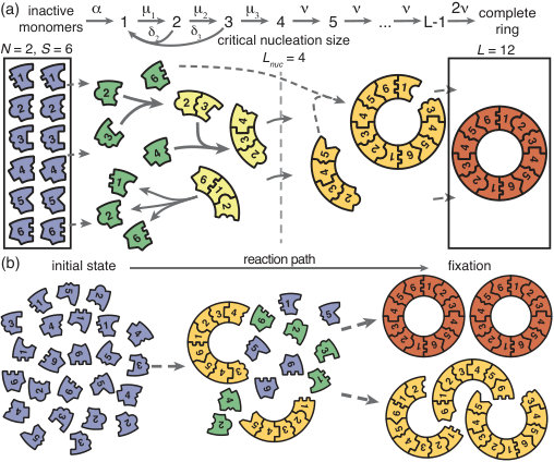 Figure 1
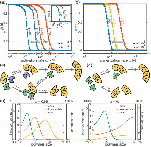 Figure 2
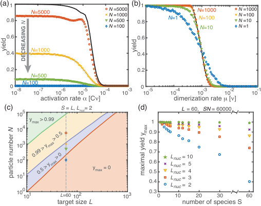 Figure 3
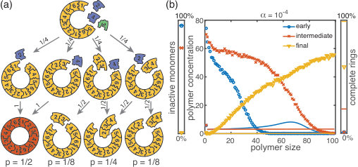 Figure 4
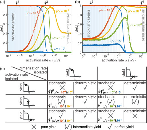 Figure 5
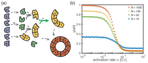 Figure 6
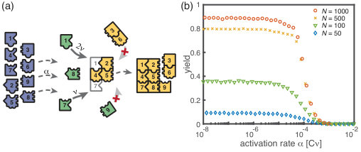 Figure 7
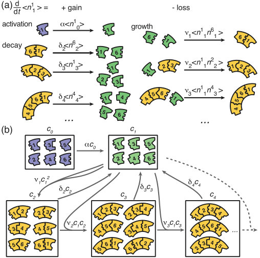 Figure 8
 Figure 9
Peer Reviews
No public reviews on file for this paper yet. If you reviewed it on a platform where reviews are public (OpenReview, ICLR, NeurIPS, ICML), you can paste yours below so the community can read it here.
Videos
No videos yet. Explain this paper in a talk, walkthrough, or lecture? Add one.
Taxonomy
TopicsModular Robots and Swarm Intelligence · Innovative Microfluidic and Catalytic Techniques Innovation · 3D Printing in Biomedical Research
**Stochastic Yield Catastrophes and Robustness in Self-Assembly **
Florian M. Gartner1⋆, Isabella R. Graf1⋆, Patrick Wilke1⋆, Philipp M. Geiger1, Erwin Frey1†
1Arnold Sommerfeld Center for Theoretical Physics (ASC) and Center for NanoScience (CeNS), Department of Physics, Ludwig-Maximilians-Universität München, Theresienstraße 37, 80333 München, Germany
⋆ F.M.G., I.R.G. and P.W. contributed equally to this work.
*†*Corresponding author: [email protected].
ABSTRACT
A guiding principle in self-assembly is that, for high production yield, nucleation of structures must be significantly slower than their growth. However, details of the mechanism that impedes nucleation are broadly considered irrelevant. Here, we analyze self-assembly into finite-sized target structures employing mathematical modeling. We investigate two key scenarios to delay nucleation: (i) by introducing a slow activation step for the assembling constituents and, (ii) by decreasing the dimerization rate. These scenarios have widely different characteristics. While the dimerization scenario exhibits robust behavior, the activation scenario is highly sensitive to demographic fluctuations. These demographic fluctuations ultimately disfavor growth compared to nucleation and can suppress yield completely. The occurrence of this stochastic yield catastrophe does not depend on model details but is generic as soon as number fluctuations between constituents are taken into account. On a broader perspective, our results reveal that stochasticity is an important limiting factor for self-assembly and that the specific implementation of the nucleation process plays a significant role in determining the yield.
1 Introduction
Efficient and accurate assembly of macromolecular structures is vital for living organisms. Not only must resource use be carefully controlled, but malfunctioning aggregates can also pose a substantial threat to the organism itself [22, 8]. Furthermore, artificial self-assembly processes have important applications in a variety of research areas like nanotechnology, biology, and medicine [43, 39, 40]. In these areas, we find a broad range of assembly schemes. For example, while a large number of viruses assemble capsids from identical protein subunits, some others, like the Escherichia virus T4, form highly complex and heterogeneous virions encompassing many different types of constituents [45, 44, 15, 26]. Furthermore, artificially built DNA structures can reach up to Gigadalton sizes and can, in principle, comprise an unlimited number of different subunits [23, 33, 11, 36]. Notwithstanding these differences, a generic self-assembly process always includes three key steps: First, subunits must be made available, e.g. by gene expression, or rendered competent for binding, e.g. by nucleotide exchange [2, 3, 38] (‘activation’). Second, the formation of a structure must be initiated by a nucleation event (‘nucleation’). Due to cooperative or allosteric effects in binding, there might be a significant nucleation barrier [3, 20, 35, 25, 16]. Third, following nucleation, structures grow via aggregation of substructures (‘growth’). To avoid kinetic traps that may occur due to irreversibility or very slow disassembly of substructures [17, 14], structure nucleation must be significantly slower than growth [45, 23, 33, 37, 21, 16]. Physically speaking, there are no irreversible reactions. However, in the biological context, self-assembly describes the (relatively fast) formation of long-lasting, stable structures. Therefore, at least part of the assembly reactions are often considered to be irreversible on the time scale of the assembly process.
In this manuscript we investigate, for a given target structure, whether the nature of the specific mechanism employed in order to slow down nucleation influences the yield of assembled product. To address this question, we examine a generic model that incorporates the key elements of self-assembly outlined above.
2 Model definition
We model the assembly of a fixed number of well-defined target structures from limited resources. Specifically, we consider a set of different species of constituents denoted by which assemble into rings of size . The cases and () are denoted as homogeneous and partially (fully) heterogeneous, respectively. The homogeneous model builds on previous work on virus capsid [3, 17], linear protein filament assembly [28, 27, 7] and aggregation and polymerization models [24]. The heterogeneous model in turn links to previous model systems used to study, for example, DNA-brick-based assembly of heterogeneous structures [30, 19, 6]. We emphasize that, even though strikingly similar experimental realizations of our model exist [11, 36, 32], it is not intended to describe any particular system. The ring structure represents a general linear assembly process involving building blocks with equivalent binding properties and resulting in a target of finite size. The main assumption in the ring model is that the different constituents assemble linearly in a sequential order. In many biological self-assembling systems like bacterial flagellum assembly or biogenesis of the ribosome subunits the assumption of a linear binding sequence appears to be justified [31, 4]. In order to test the validity of our results beyond these constraints we also perform stochastic simulations of generalized self-assembling systems that do not obey a sequential binding order: i) by explicitly allowing for polymer-polymer bindings and ii) by considering the assembly of finite sized squares that grow independently in two dimensions (see Figs. 6 and 7).
The assembly process starts with inactive monomers of each species. We use to denote the initial concentration of each monomer species, where is the reaction volume. Monomers are activated independently at the same per capita rate , and, once active, are available for binding. Binding takes place only between constituents of species with periodically consecutive indices, for example and or and (leading to structures such as for ); see Fig. 1. To avoid ambiguity, we restrict ring sizes to integer multiples of the number of species . Furthermore, we neglect the possibility of incorrect binding, e.g. species 1 binding to 3 or . Polymers, i.e., incomplete ring structures, grow via consecutive attachment of monomers. For simplicity, polymer-polymer binding is disregarded at first, as it is typically assumed to be of minor importance [45, 3, 30, 18]. To probe the robustness of the model, later we consider an extended model including polymer-polymer binding for which the results are qualitatively the same (see Fig. 6 and the discussion). Furthermore, it has been observed that nucleation phenomena play a critical role for self-assembly processes [23, 37, 33, 3]. So it is in general necessary to take into account a critical nucleation size, which marks the transition between slow particle nucleation and the faster subsequent structure growth [28, 25, 29, 30]. We denote this critical nucleation size by , which in terms of classical nucleation theory corresponds to the structure size at which the free energy barrier has its maximum. For attachment of monomers to existing structures and decay of structures (reversible binding) into monomers take place at size-dependent reaction rates and , respectively (Fig. 1). Here, we focus on identical rates and . A discussion of the general case is given in the Supplementary Information [1]. Above the nucleation size, polymers grow by attachment of monomers with reaction rate per binding site. As we consider successfully nucleated structures to be stable on the observational time scales, monomer detachment from structures above the critical nucelation size is neglected (irreversible binding) [30, 3]. Complete rings neither grow nor decay (absorbing state).
We investigate two scenarios for the control of nucleation speed, first separately and then in combination. For the ‘activation scenario’ we set (all binding rates are equal) and control the assembly process by varying the activation rate . For the ‘dimerization scenario’ all particles are inherently active () and we control the assembly process by varying the dimerization rate (we focus on ). It has been demonstrated previously in [3] and [9, 16, 29] that either a slow activation or a slow dimerization step are suitable in principle to retard nucleation and favour growth of the structures over the initiation of new ones. We quantify the quality of the assembly process in terms of the assembly yield, defined as the number of successfully assembled ring structures relative to the maximal possible number . Yield is measured when all resources have been used up and the system has reached its final state. We do not discuss the assembly time in this manuscript, however, in the Supplementary Information [1] we show typical trajectories for the time evolution of the yield in the activation and dimerization scenario. If the assembly product is stable (absorbing state), the yield can only increase with time. Consequently, the final yield constitutes the upper limit for the yield irrespective of additional time constraints. Therefore, the final yield is an informative and unambiguous observable to describe the efficiency of the assembly reaction.
We simulated our system both stochastically via Gillespie’s algorithm [12] and deterministically as a set of ordinary differential equations corresponding to chemical rate equations (see Supplementary Information [1]).
3 Results
3.1 Deterministic behavior in the macroscopic limit.
First, we consider the macroscopic limit, , and investigate how assembly yield depends on the activation rate (activation scenario) and the dimerization rate (dimerization scenario) for . Here, the deterministic description coincides with the stochastic simulations (Fig. 2(a) and (b)). For both high activation and high dimerization rates, yield is very poor. Upon decreasing either the activation rate (Fig. 2(a)) or the dimerization rate (Fig. 2(b)), however, we find a threshold value, or , below which a rapid transition to the perfect yield of 1 is observed both in the deterministic and stochastic simulation. By exploiting the symmetries of the system with respect to relabeling of species, one can show that, in the deterministic limit, the behavior is independent of the number of species (for fixed and , see Supplementary Information [1]). Consequently, all systems behave equivalently to the homogeneous system and yield becomes independent of in this limit. Note, however, that equivalent systems with differing have different total numbers of particles and hence assemble different total numbers of rings.
Decreasing the activation rate reduces the concentration of active monomers in the system. Hence growth of the polymers is favored over nucleation, because growth depends linearly on the concentration of active monomers while nucleation shows a quadratic dependence. Likewise, lower dimerization rates slow down nucleation relative to growth. Both mechanisms therefore restrict the number of nucleation events, and ensure that initiated structures can be completed before resources become depleted (see Fig. 2(c) and (d)).
Mathematically, the deterministic time evolution of the polymer size distribution is described by an advection-diffusion equation [9, 41] with advection and diffusion coefficients depending on the instantaneous concentration of active monomers (see Supplementary Information [1]). Solving this equation results in the wavefront of the size distribution advancing from small to large polymer sizes (Fig. 2(e)). Yield production sets in as soon as the distance travelled by this wavefront reaches the maximal ring size . Exploiting this condition, we find that in the deterministic system for , a non-zero yield is obtained if either the activation rate or the dimerization rate remains below a corresponding threshold value, i.e. if or , where
[TABLE]
(see Supplementary Information [1]) with proportionality constants and . These relations generalize previous results [29] to finite activation rates and for heterogeneous systems. A comparison between the threshold values given by Eq. 1 and the simulated yield curves is shown in Fig. 2(a,b). The relations highlight important differences between the two scenarios (where and , respectively): While decreases cubically with the ring size , does so only quadratically. Furthermore, the threshold activation rate increases with the initial monomer concentration . Consequently, for fixed activation rate, the yield can be optimized by increasing . In contrast, the threshold dimerization rate is independent of and the yield curves coincide for . Finally, if is finite and , the interplay between the two slow-nucleation scenarios may lead to enhanced yield. This is reflected by the factor in , and we will come back to this point later when we discuss the stochastic effects.
In summary, for large particle numbers (), perfect yield can be achieved in two different ways, independently of the heterogeneity of the system - by decreasing either the activation rate (activation scenario) or the dimerization rate (dimerization scenario) below its respective threshold value.
3.2 Stochastic effects in the case of reduced resources.
Next, we consider the limit where the particle number becomes relevant for the physics of the system. In the activation scenario, we find a markedly different phenomenology if resources are sparse. Figure 3(a) shows the dependence of the average yield on the activation rate for different, low particle numbers in the completely heterogeneous case () 111Here, we restrict our discussion to the average yield. The error of the mean is negligible due to the large number of simulations used to calculate the average yield. Still, due to the randomness in binding and activation, the yield can differ between simulations. A figure with the average yield and its standard deviation is shown in the Supplementary Information [1]. For very low and very high average yield, the standard deviation has to be small due to the boundedness of the yield. For intermediate values of the average, the standard deviation is highest but still small compared to the average yield. Thus, the average yield is meaningful for the essential understanding of the assembly process.. Whereas the deterministic theory predicts perfect yield for small activation rates, in the stochastic simulation yield saturates at an imperfect value . Reducing the particle number decreases this saturation value until no finished structures are produced (). The magnitude of this effect strongly depends on the size of the target structure if the system is heterogeneous. Fig. 3(c) shows a diagram characterizing different regimes for the saturation value of the yield, , in dependence of the particle number and the size of the target structure for fully heterogeneous systems . We find that the threshold particle number necessary to obtain a fixed yield increases nonlinearly with the target size . For the depicted range of , the dependence of the threshold for nonzero yield, , on can approximately be described by a power-law: , with exponent for . Consequently, for already more than rings must be assembled in order to obtain a yield larger than zero. In the Supplementary Information [1] we included two additional plots that show the dependence of on for fixed and the dependence on for fixed , respectively. The suppression of the yield is caused by fluctuations (see explanation below) and is not captured by a deterministic description. Because these stochastic effects can decrease the yield from a perfect value in a deterministic description to zero (see Fig. 3(a)), we term this effect ‘stochastic yield catastrophe’.
For fixed target size and fixed maximum number of target structures , increases with decreasing number of species, see Fig. 3(d). In the fully homogeneous case, , a perfect yield of 1 is always achieved for . The decrease of the maximal yield with the number of species thus suggests that, in order to obtain high yield, it is beneficial to design structures with as few different species as possible. In large part this effect is due to the constraint , whereby the more homogeneous systems (small ) require larger numbers of particles per species and, correspondingly, exhibit less stochasticity. If is fixed instead of , the yield still initially decreases with increasing number of species but then quickly reaches a stationary plateau and gets independent of for , see Supplementary Information [1]. Moreover, increasing the nucleation size , and with it the reversibility of binding, also increases , see Fig. 3(d). This indicates that, beside heterogeneity of the target structure, irreversibility of binding on the relevant time scale makes the system susceptible to stochastic effects.
The stochastic yield catastrophe is mainly attributable to fluctuations in the number of active monomers. In the deterministic (mean-field) equation the different particle species evolve in balanced stoichiometric concentrations. However, if activation is much slower than binding, the number of active monomers present at any given time is small, and the mean-field assumption of equal concentrations is violated due to fluctuations (for ). Activated monomers then might not fit any of the existing larger structures and would instead initiate new structures. Figure 4(a) illustrates this effect and shows how fluctuations in the availability of active particles lead to an enhanced nucleation and, correspondingly, to a decrease in yield. Due to the effective enhancement of the nucleation rate, the resulting polymer size distribution has a higher amplitude than that predicted deterministically (Fig. 4(b)) and the system is prone to depletion traps. A similar broadening of the size distribution has been reported in the context of stochastic coagulation-fragmentation of identical particles [5].
In the dimerization scenario, in contrast, there is no stochastic activation step. All particles are available for binding from the outset. Consequently, stochastic effects do not play an essential role in the dimerization scenario and perfect yield can be reached robustly for all system sizes, regardless of the number of species (Fig. 3(b)).
3.3 Non-monotonic yield curves for a combination of slow dimerization and activation.
So far, the two implementations of the ‘slow nucleation principle’ have been investigated separately. Surprisingly, we observe counter-intuitive behavior in a mixed scenario in which both dimerization and activation occur slowly (i.e., , ). Figure 5 shows that, depending on the ratio , the yield can become a non-monotonic function of . In the regime where is large, nucleation is dimerization-limited; therefore activation is irrelevant and the system behaves as in the dimerization scenario for . Upon decreasing we then encounter a second regime, where activation and dimerization jointly limit nucleation. The yield increases due to synergism between slow dimerization and activation (see dependence of , Eq. 1), whilst the average number of active monomers is still high and fluctuations are negligible. Finally, a stochastic yield catastrophe occurs if is further reduced and activation becomes the limiting step. This decline is caused by an increase in nucleation events due to relative fluctuations in the availability of the different species (“fluctuations between species”). This contrasts the deterministic description where nucleation is always slower for smaller activation rate. Depending on the ratio , the ring size and the particle number , maximal yield is obtained either in the dimerization-limited (red curves, Fig. 5), activation-limited (blue curve, Fig. 5(b)) or intermediate regime (green and orange curves).
3.4 Robustness of the results to model modifications.
In our model, the reason for the stochastic yield catastrophe is that - due to fluctuations between species - the effective nucleation rate is strongly enhanced. Hence, if binding to a larger structure is temporarily impossible, activated monomers tend to initiate new structures, causing an excess of structures that ultimately cannot be completed. Natural questions that arise are whether i) relaxing the constraint that polymers cannot bind other polymers or ii) abandoning the assumption of a linear assembly path, will resolve the stochastic yield catastrophe. To answer these questions, we performed stochastic simulations for extensions of our model system showing that the stochastic yield catastrophe indeed persists.
We start by considering the ring model from the previous section but take polymer-polymer binding into account in addition to growth via monomer attachment (Fig.6). In detail, we assume that two structures of arbitrary size (and with combined length ) bind at rate if they fit together, i.e. if the left (right) end of the first structure is periodically continued by the right (left) end of the second one. Realistically, the rate of binding between two structures is expected to decrease with the motility and thus the sizes of the structures. In order to assess the effect of polymer-polymer binding, we focus on the worst case where the rate for binding is independent of the size of both structures. If a stochastic yield catastrophe occurs for this choice of parameters, we expect it to be even more pronounced in all the “intermediate cases”. Fig. 6 shows the dependence of the yield on the activation rate in the polymer-polymer model. As before, yield increases below a critical activation rate and then saturates at an imperfect value for small activation rates. Decreasing the number of particles per species, decreases this saturation value. Compared to the original model, the stochastic yield catastrophe is mitigated but still significant: For structures of size , yield saturates at around for particles per species and at around for particles per species. We thus conclude that polymer-polymer binding indeed alleviates the stochastic yield catastrophe but does not resolve it. Since binding only happens between consecutive species, structures with overlapping parts intrinsically can not bind together and depletion traps continue to occur. Taken together, also in the extended model, fluctuations in the availability of the different species lead to an excess of intermediate-sized structures that get kinetically trapped due to structural mismatches. Note that in the extreme case of , incomplete polymers can always combine into 1 final ring structure so that in this case yield is always 1. Analogously, for high activation rates yield is improved for compared to (Fig. 6 b).
Kinetic trapping due to structural mismatches can occur in every (partially) irreversible heterogeneous assembly process with finite-sized target structure and limited resources. From our results, we thus expect a stochastic yield catastrophe to be common to such systems. In order to further test this hypothesis, we simulated another variant of our model where finite sized squares assemble via monomer attachment from a pool of initially inactive particles, see Fig 7 . In contrast to the original model, the assembled structures are non-periodic and exhibit a non-linear assembly path where structures can grow independently in two dimensions. While the ring model assumes a sequential order of binding of the monomers, the square allows for a variety of distinct assembly paths that all lead to the same final structure. Note that, because of the absence of periodicity the square model is only well defined for the completely heterogeneous case. Figure 7 depicts the dependence of the yield on the activation rate for a square of size . Also in this case, we find that the yield saturates at an imperfect value for small activation rates. Hence, we showed that the stochastic yield catastrophe is not resolved neither by accounting for polymer-polymer combination nor by considering more general assembly processes with multiple parallel assembly paths. This observation supports the general validity of our findings and indicates that stochastic yield catastrophes are a general phenomenon of (partially) irreversible and heterogeneous self-assembling systems that occur if particle number fluctuations are non-negligible.
4 Discussion
Our results show that different ways to slow down nucleation are indeed not equivalent, and that the explicit implementation is crucial for assembly efficiency. Susceptibility to stochastic effects is highly dependent on the specific scenario. Whereas systems for which dimerization limits nucleation are robust against stochastic effects, stochastic yield catastrophes can occur in heterogeneous systems when resource supply limits nucleation. The occurrence of stochastic yield catastrophes is not captured by the deterministic rate equations, for which the qualitative behavior of both scenarios is the same. Therefore, a stochastic description of the self-assembly process, which includes fluctuations in the availability of the different species, is required. The interplay between stochastic and deterministic dynamics can lead to a plethora of interesting behaviors. For example, the combination of slow activation and slow nucleation may result in a non-monotonic dependence of the yield on the activation rate. While deterministically, yield is always improved by decreasing the activation rate, stochastic fluctuations between species strongly suppress the yield for small activation rate by effectively enhancing the nucleation speed. This observation clearly demonstrates that a deterministically slow nucleation speed is not sufficient in order to obtain good yield in heterogeneous self-assembly. For example, a slow activation step does not necessarily result in few nucleation events although deterministically this behavior is expected. Thus, our results indicate that the slow nucleation principle has to be interpreted in terms of the stochastic framework and have important implications for yield optimization.
We showed that demographic noise can cause stochastic yield catastrophes in heterogeneous self-assembly. However, other types of noise, such as spatiotemporal fluctuations induced by diffusion, are also expected to trigger stochastic yield catastrophes. Hence, our results have broad implications for complex biological and artificial systems, which typically exhibit various sources of noise. We characterize conditions under which stochastic yield catastrophes occur, and demonstrate how they can be mitigated. These insights could usefully inform the design of experiments to circumvent yield catastrophes: In particular, while slow provision of constituents is a feasible strategy for experiments, it is highly susceptible to stochastic effects. On the other hand, irrespective of its robustness to stochastic effects, the experimental realization of the dimerization scenario relies on cooperative or allosteric effects in binding, and may therefore require more sophisticated design of the constituents [34, 42]. Our theoretical analysis shows that stochasticity can be alleviated either by decreasing heterogeneity (presumably lowering realizable complexity) or by increasing reversibility (potentially requiring fine-tuning of bond strengths and reducing the stability of the assembly product). Alternative approaches to control stochasticity include the promotion of specific assembly paths [30, 10] and the control of fluctuations [13]. One possibility to test these ideas and the ensuing control strategies could be via experiments based on DNA origami. Instead of building homogeneous ring structures as in Ref. [36], one would have to design heterogeneous ring structures made from several different types of constituents with specified binding properties. By varying the opening angle of the “wedges” (and thus the preferred number of building blocks in the ring) and/or the number of constituents, both the target structure size as well as the heterogeneity of the target structure could be controlled.
Moreover, the ideas presented in this manuscript are relevant for the understanding of intracellular self-assembly. In cells, provision of building blocks is typically a gradual process, as synthesis is either inherently slow or an explicit activation step, such as phosphorylation, is required. In addition, the constituents of the complex structures assembled in cells are usually present in small numbers and subject to diffusion. Hence, stochastic yield catastrophes would be expected to have devastating consequences for self-assembly, unless the relevant cellular processes use elaborate control mechanisms to circumvent stochastic effects. Further exploration of these control mechanisms should enhance the understanding of self-assembly processes in cells and help improve synthesis of complex nanostructures.
5 Methods and Materials
Here we show the derivation of Eq. 1 in the main text, giving the threshold values for the rate constants below which finite yield is obtained. The details can be found in the Supplementary Information [1].
5.1 Master equation and chemical rate equations
We start with the general Master equation and derive the chemical rate equations (deterministic/mean-field equations) for the heterogeneous self-assembly process. We renounce to show the full Master equation here but instead state the system that describes the evolution of the first moments. To this end, we denote the random variable that describes the number of polymers of size and species in the system at time by with and . The species of a polymer is defined by the species of the respective monomer at its left end. Furthermore, and denote the number of inactive and active monomers of species , respectively, and the number of complete rings. We signify the reaction rate for binding of a monomer to a polymer of size by . denotes the activation rate and the decay rate of a polymer of size . By we indicate (ensemble) averages. The system governing the evolution of the first moments (the averages) of the is then given by:
[TABLE]
The different terms of this equation are illustrated graphically in Figure 8. The first equation describes loss of inactive particles due to activation at rate . Eq. (2b) gives the temporal change of the number of active monomers that is governed by the following processes: activation of inactive monomers at rate , binding of active monomers to the left or to the right end of an existing structure of size at rate , and decay of below-critical polymers of size into monomers at rate (disassembly).
Equations (2c) and (2d) describe the dynamics of dimers and larger polymers of size , respectively. The terms account for reactions of polymers with active monomers (polymerization) as well as decay in the case of below-critical polymers (disassembly). The indicator function equals if the condition is satisfied and [math] otherwise. Note that a polymer of size can grow by attaching a monomer to its left or to its right end whereas the formation of a dimer of a specific species is only possible via one reaction pathway (dimerization reaction). Finally, polymers of length – the complete ring structures – form an absorbing state and, therefore, include only the respective gain terms (cf. Eq 2e).
We simulated the Master equation underlying Eq. (2) stochastically using Gillespie’s algorithm. For the following deterministic analysis, we neglect correlations between particle numbers , which is valid assumption for large particle numbers. Then the two-point correlator can be approximated as the product of the corresponding mean values (mean-field approximation)
[TABLE]
Furthermore, for the expectation values it must hold
[TABLE]
because all species have equivalent properties (there is no distinct species) and hence the system is invariant under relabelling of the upper index. By
[TABLE]
we denote the concentration of any monomer or polymer species of size , where is the reaction volume. Due to the symmetry formulated in Eq. (4), the heterogeneous assembly process decouples into a set of identical and independent homogeneous assembly processes in the deterministic limit. The corresponding homogeneous system then is described by the following set of equations that is obtained by applying (3), (4) and (5) to (2)
[TABLE]
The rate constants in Eq. (6) and (2) differ by a factor of . For convenience, we use however the same symbol in both cases. The rate constants in Eq. (6) can be interpreted in the usual units . Due to the symmetry, the yield, which is given by the quotient of the number of completely assembled rings and the maximum number of complete rings, becomes independent of the number of species
[TABLE]
Hence, it is enough to study the dynamics of the homogeneous system, Eq. (6), to identify the condition under which non zero yield is obtained.
5.2 Effective description by an advection-diffusion equation
The dynamical properties of the evolution of the polymer-size distribution become evident if the set of ODEs (6) is rewritten as a partial differential equation. This approach was previously described in the context of virus capsid assembly [45, 29].
For simplicity, we restrict ourselves to the case and let and . Then, for the polymers with we have
[TABLE]
As a next step, we approximate the index indicating the length of the polymer as a continuous variable and define . By we denote the concentration of active monomers in the following to emphasize their special role. Formally expanding the right-hand side of Eq. (8) in a Taylor series up to second order
[TABLE]
one arrives at the advection-diffusion equation with both advection and diffusion coefficients depending on the concentration of active monomers
[TABLE]
Equation (10) can be written in the form of a continuity equation with flux . The flux at the left boundary equals the influx of polymers due to dimerization of free monomers . This enforces a Robin boundary condition at
[TABLE]
At we set an absorbing boundary so that completed structures are removed from the system. The time evolution of the concentration of active monomers is given by
[TABLE]
The terms on the right-hand side account for activation of inactive particles, dimerization, and binding of active particles to polymers (polymerization).
Qualitatively, Eq. (10) describes a profile that emerges at from the boundary condition Eq. (11) moves to the right with time-dependent velocity due to the advection term, and broadens with a time-dependent diffusion coefficient . In the Supplementary Information [1] we show how the full solution of Eqs. (10) and (11) can be found assuming knowledge of . Here, we focus only on the derivation of the threshold activation rate and threshold dimerization rate that mark the onset of non-zero yield.
Yield production starts as soon as the density wave reaches the absorbing boundary at . Therefore, finite yield is obtained if the sum of the advectively travelled distance and the diffusively travelled distance exceeds the system size
[TABLE]
According to Eq. (10), and , giving as condition for the onset of finite yield
[TABLE]
where the last approximation is valid for large .
In order to obtain we derive an effective two-component system that governs the evolution of . To this end, we denote the total number of polymers in Eq. (12) by (as long as yield is zero the upper boundary is irrelevant and we can consider ). Eq. (12) then reads
[TABLE]
and the dynamics of is determined from the boundary condition, Eq. (11)
[TABLE]
Measuring and in units of the initial monomer concentration and time in units of the equations are rewritten in dimensionless units as
[TABLE]
where and . Eq. (17) describes a closed two-component system for the concentration of active monomers and the total concentration of polymers . It describes the dynamics exactly as long as yield is zero. In order to evaluate the condition (14) we need to determine the integral over as a function of and
[TABLE]
To that end, we proceed by looking at both scenarios separately. The numerical analysis, confirming our analytic results, is given in the Supplementary Information [1].
5.3 Dimerization scenario
The activation rate in the dimerization scenario is , and instead of the term in , we set the initial condition (and ). Furthermore, and we can neglect the term proportional to in . As a result,
[TABLE]
Solving this equation for as a function of using the initial condition , the totally travelled distance of the wave is determined to be
[TABLE]
where for the evaluation of the integral we used the substitution .
5.4 Activation scenario
In the activation scenario, yield sets in only if the activation rate and thus the effective nucleation rate is slow. As a result, in addition to , we can again neglect the term proportional to in . This time, however, we have to keep the term . As a next step, we assume that is much smaller than the remaining terms on the right-hand side, and . This assumption might seem crude at first sight but is justified a posteriori by the solution of the equation (see Supplementary Information [1]). Hence, we get the algebraic equation . Using it to solve for , and then to determine , the totally travelled distance of the wave is deduced as
[TABLE]
Taken together, we therefore obtain two conditions out of which one must be fulfilled in order to obtain finite yield
[TABLE]
where and are numerical factors, and and . This verifies Eq. (1) in the main text.
6 Acknowledgments
We thank Nigel Goldenfeld for a stimulating discussion, and Raphaela Geßele and Laeschkir Hassan for helpful feedback on the manuscript. This research was supported by the German Excellence Initiative via the program ‘NanoSystems Initiative Munich’(NIM) and was funded by the Deutsche Forschungsgemeinschaft (DFG, German Research Foundation) under Germany’s Excellence Strategy – EXC-2094 – 390783311. F.M.G. and I.R.G. are supported by a DFG fellowship through the Graduate School of Quantitative Biosciences Munich (QBM). We also gratefully acknowledge financial support by the DFG Research Training Group GRK2062 (Molecular Principles of Synthetic Biology). Finally, E.F. thanks the Aspen Center for Physics, which is supported by National Science Foundation grant PHY-1607611, for their hospitality and inspiring discussions with colleagues.
The reference list from the paper itself. Each links out to its DOI / PubMed record.
- 11. See Supplementary Information.
- 22. Bruce Alberts, Alexander Johnson, Julian Lewis, David Morgan, Martin Raff, Keith Roberts, Peter Walter, John Wilson, and Tim Hunt. Molecular Biology of the Cell . Garland Science, 2015.
- 33. Chao Chen, C Cheng Kao, and Bogdan Dragnea. Self-assembly of brome mosaic virus capsids: insights from shorter time-scale experiments. The Journal of Physical Chemistry A , 112(39):9405–9412, 2008.
- 44. Fabienne FV Chevance and Kelly T Hughes. Coordinating assembly of a bacterial macromolecular machine. Nature Reviews Microbiology , 6(6):455, 2008.
- 55. Maria R D’Orsogna, Qi Lei, and Tom Chou. First assembly times and equilibration in stochastic coagulation-fragmentation. The Journal of chemical physics , 143(1):014112, 2015.
- 66. Maria R D’Orsogna, Bingyu Zhao, Bijan Berenji, and Tom Chou. Combinatoric analysis of heterogeneous stochastic self-assembly. The Journal of chemical physics , 139(12):121918, 2013.
- 77. MR D’Orsogna, Greg Lakatos, and Tom Chou. Stochastic self-assembly of incommensurate clusters. The Journal of chemical physics , 136(8):084110, 2012.
- 88. D Allan Drummond and Claus O Wilke. The evolutionary consequences of erroneous protein synthesis. Nature Reviews Genetics , 10(10):715–724, 2009.