Adaptive Function-on-Scalar Regression with a Smoothing Elastic Net
Ardalan Mirshani, Matthew Reimherr

TL;DR
This paper introduces AFSSEN, a novel adaptive Elastic Net approach for high-dimensional function-on-scalar regression that effectively selects predictors and ensures smooth estimates within a Hilbert space framework.
Contribution
The paper develops a new regularization method combining functional norms for simultaneous variable selection and smoothing in a high-dimensional setting.
Findings
AFSSEN outperforms existing methods in prediction accuracy.
It achieves better variable selection with fewer false positives.
Theoretical properties include a functional oracle property.
Abstract
This paper presents a new methodology, called AFSSEN, to simultaneously select significant predictors and produce smooth estimates in a high-dimensional function-on-scalar linear model with a sub-Gaussian errors. Outcomes are assumed to lie in a general real separable Hilbert space, H, while parameters lie in a subspace known as a Cameron Martin space, K, which are closely related to Reproducing Kernel Hilbert Spaces, so that parameter estimates inherit particular properties, such as smoothness or periodicity, without enforcing such properties on the data. We propose a regularization method in the style of an adaptive Elastic Net penalty that involves mixing two types of functional norms, providing a fine tune control of both the smoothing and variable selection in the estimated model. Asymptotic theory is provided in the form of a functional oracle property, and the paper concludes…
Click any figure to enlarge with its caption.
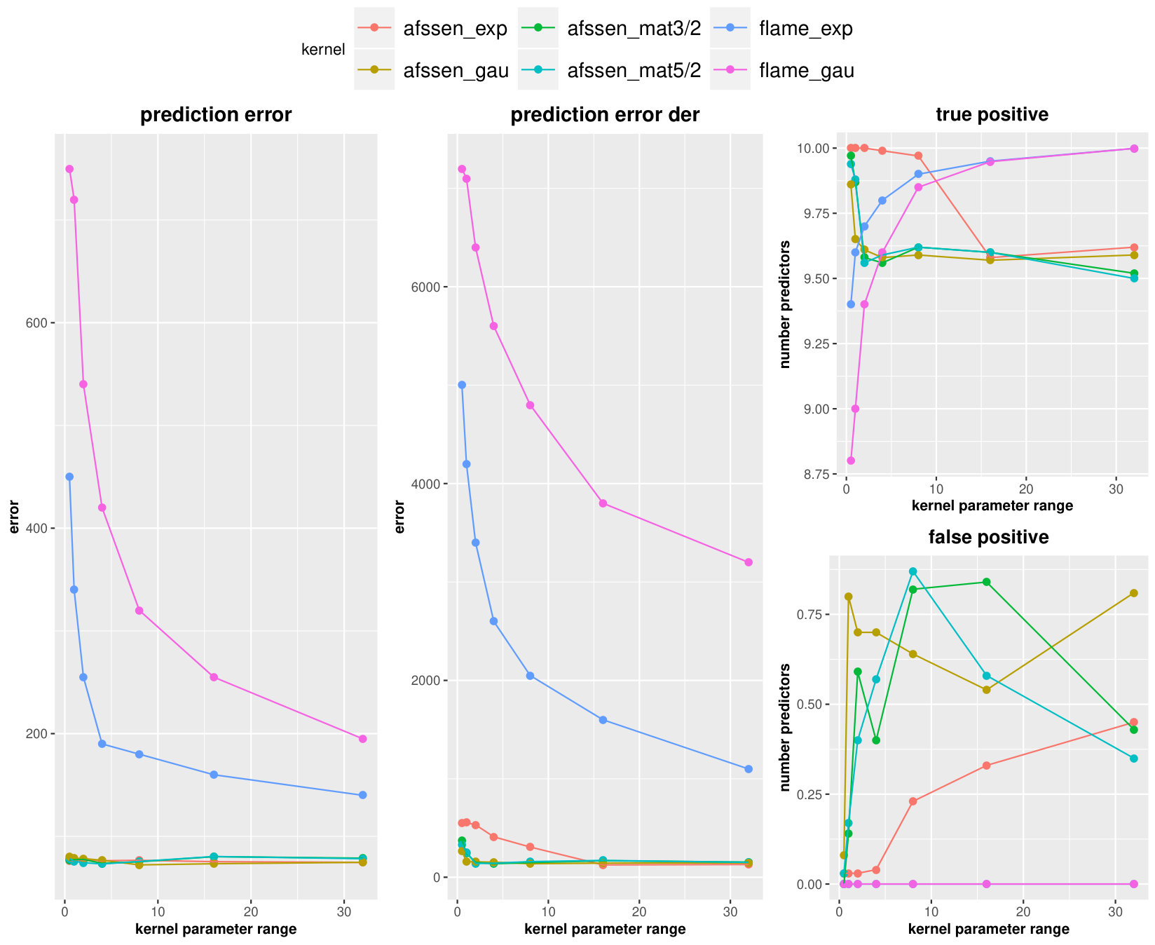 Figure 1
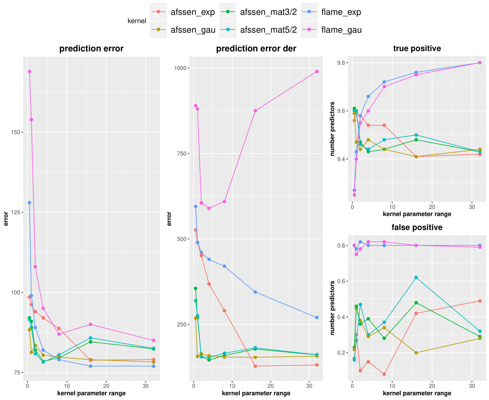 Figure 2
Peer Reviews
No public reviews on file for this paper yet. If you reviewed it on a platform where reviews are public (OpenReview, ICLR, NeurIPS, ICML), you can paste yours below so the community can read it here.
Videos
No videos yet. Explain this paper in a talk, walkthrough, or lecture? Add one.
Adaptive Function-on-Scalar Regression with a Smoothing Elastic Net
Ardalan Mirshani
Department of Statistics
The Pennsylvania State University
University Park, PA 16802
&Matthew Reimherr
Department of Statistics
The Pennsylvania State University
University Park, PA 16802
[email protected] Corresponding Author
Abstract
This paper presents a new methodology, called AFSSEN, to simultaneously select significant predictors and produce smooth estimates in a high-dimensional function-on-scalar linear model with a sub-Gaussian errors. Outcomes are assumed to lie in a general real separable Hilbert space, , while parameters lie in a subspace known as a Cameron Martin space, , which are closely related to Reproducing Kernel Hilbert Spaces, so that parameter estimates inherit particular properties, such as smoothness or periodicity, without enforcing such properties on the data. We propose a regularization method in the style of an adaptive Elastic Net penalty that involves mixing two types of functional norms, providing a fine tune control of both the smoothing and variable selection in the estimated model. Asymptotic theory is provided in the form of a functional oracle property, and the paper concludes with a simulation study demonstrating the advantage of using AFSSEN over existing methods in terms of prediction error and variable selection.
KEYWORDS: Variable Selection, Functional Data Analysis, Hilbert Space, Elastic Net, Smooth Estimate, Reproducing Kernel Hilbert Space , Oracle Property
1 Introduction
In recent years, rapid advances in data gathering technologies and new complex modern studies have presented substantial challenges for extracting information from increasingly large and sophisticated data sets. Functional data analysis, FDA, is a branch of statistics for conducting statistical inferences on the complicated objects specially in high dimensional spaces (Ramsay and Silverman, 2007; Hsing and Eubank, 2015; Kokoszka and Reimherr, 2017). In addition, the emergence of inexpensive genotyping technologies has produced a substantial need for tools capable of handling large numbers of scalar predictors (Bierut et al., 2006; Scott et al., 2007; Repapi et al., 2010; Hebiri et al., 2011; Algamal and Lee, 2015; Craig et al., 2018). In this paper, we consider the function-on-scalar regression problem when the number of predictors is much larger than the number of subjects/units. We present a new approach, called AFSSEN, for Adaptive Function-on-Scalar Smoothing Elastic Net, which can separately control the smoothness of the underlying functional parameter estimates as well as select important predictors.
As in classic statistical analyses, the functional linear model, FLM, is one the principle modeling tools when working with functional data (Morris, 2015). In these cases, at least one of the outcomes or predictors are functional (Reiss et al., 2010). When the number of predictors is fixed, then techniques for fitting FLM and their statistical properties are now well understood (Morris, 2015; Kokoszka and Reimherr, 2017) in low dimensional FLM, However, in high dimensional cases where the number of predictors are relatively larger than the number of statistical units, little work has been done which most of them are for Scalar-on-Function settings (Matsui and Konishi (2011) ; Gertheiss et al. (2013); Lian (2013) ; Fan et al. (2015)).
In Function-on-Scalar regression, which is the problem we consider, Chen et al. (2016) considered a functional least squares with a Minimax Concave Penalty, MCP (Zhang et al., 2010) with fixed number of predictors. A pre-whitening technique was used to exploit the within function dependence of the outcomes. Barber et al. (2017) presented the Function-on-Scalar LASSO, FSL, which combines a functional least squares with an penalty introduced in a separable Hilbert Space . Since FSL is a convex optimization problem, it is computationally efficient even with a large number of predictors (). Additionally, FSL estimates achieve optimal convergence rates, but as with traditional LASSO, these estimates suffer from an asymptotic bias and do not achieve the functional oracle property. Fan and Reimherr (2017) suggested Adaptive Function-on-Scalar LASSO, AFSL, which uses a functional least squares with an adaptive penalty to reduce the bias problem in FSL. They showed AFSL is computationally as efficient as FSL, but achieves a strong functional oracle property. However, AFSL provides limited control of the smoothness of the functional parameter estimates, which can affect on the prediction error. Parodi and Reimherr (2017) developed the Functional Linear Adaptive Mixed Estimation, FLAME, which simultaneously selects important predictors and estimates the smooth parameters. They assume that while the data lie in a general real separable Hilbert space, , the model parameters lie in a Reproducing Kernel Hilbert Space (RKHS), . The RKHS is a subspace of , which can be identified with a linear operator, They demonstrated that FLAME achieved a weak functional oracle property, meaning it recovered the correct support with probability tending to one and FLAME estimator is equivalent to the oracle estimator only on certain nice projections. To show that FLAME achieved the strong oracle property required stronger structural assumptions. In their framework, they used a coordinate descent algorithm which made it computationally very efficient.
The main obstacle for FLAME is having to simultaneously control the smoothness and sparsity with a single penalty and tuning parameter. In particular, a tuning parameter value that practically works well for smoothing may not work well for variable selection, and vice versa. To address this issue we propose a method that more carefully controls smoothing and sparsity separately. We assume the data live in an arbitrary Hilbert space, , but that some linear constraint of the parameters are enforced to lie in a Cameron-Martin space, CMS, . CMS are closely related to Reproducing Kernel Hilbert Spaces, RKHS, when , and the two terms are often used interchangeably (Bogachev, 1998). However, since our will be more general, we refrain from using the term RKHS to avoid confusion. In our approach, AFSSEN, we use an idea similar to the scalar adaptive elastic net penalty (Zou and Hastie, 2005; Zou, 2006), but for functional data. In particular, AFSSEN exploits a combination of a penalized functional least squares and an adaptive smoothing elastic net penalty containing a term in for variable selection and a separate term in for controlling the smoothness of the estimated parameters. The AFSSEN parameter estimates inherit the nature properties of the kernel function of , such as smoothness or periodicity. We also show that AFSSEN enjoys better mathematical properties than AFSL or FLAME, even when relaxing the Gaussian error assumption to -subgaussian. In particular, we show that AFSSEN achieves a strong oracle property in both and the strong norm . We also provide a very fast coordinate descent algorithm in the R programming language (R Core Team, 2018), whose backend is written in C++ (Eddelbuettel and François, 2011).
The remainder of the paper is organized as follows. In Section 2 we propose some primary materials and main assumptions for the results presented in next sections. Section 3 provides the framework and demonstrates the strong oracle property for AFSSEN under some non-strong assumptions. In section 4 we introduce the implementation and numerical illustration including the coordinate descent algorithm and practical considerations. A simulation study with a discussion on comparing the performance of AFSSEN and FLAME in two different smooth and rough scenarios is given in section 5. You can see a conclusion in Section 6. All mathematical proofs and derivations can be found in the supplemental.
2 Background and Methodology
Throughout this paper we consider is a real separable Hilbert space with inner product and induced norm . Let be a compact, positive definite, self-adjoint linear operator, meaning when , for all , and it has a finite trace. According to the spectral theorem (Dunford and Schwartz, 1963), we can decompose K as , where is an orthonormal basis of and is a positive sequence of real numbers. The eigenvalues, and eigenfunctions, of induce a subspace of , denoted , called the Cameron-Martin (Bogachev, 1998) space defined as
[TABLE]
Equivalently, can be viewed as the image (Bogachev, 1998). Then is also a Hilbert space under the inner product . The most commonly encountered Hilbert space in FDA is which is the space of real valued square integrable functions over with corresponding norm . When and is an integral operator with kernel , then is isomorphic to a Reproducing Kernel Hilbert Space (Berlinet and Thomas-Agnan, 2011).
In previous works (Fan and Reimherr, 2017; Parodi and Reimherr, 2017), the modelling noise was assumed to be a Gaussian process. In this paper, we relax this assumption by consider a -subgaussian noise, which, to the best of our knowledge, has not been considered before in functional data models. A mean zero random element in is called -subgaussian if
[TABLE]
where is a covariance operator in (Buldygin and Kozachenko, 1980; Antonioni, 1997). In other words, the moment generating function of the is dominated, uniformly across , by the moment generating function of a Gaussian process with covariance . This is a convenient assumption as it provides the necessary tail probability inequalities (Hsu et al., 2012) without making explicit assumptions on the distribution of . In particular, one can see a Gaussian process in with covariance operator will be a -subgaussian process in (Antonioni, 1997).
We now introduce our primary modelling assumptions.
Assumption 1**.**
Let Y_{n}\in{\mathbb{H}}\ for satisfy
[TABLE]
where is the design matrix with standardized columns and are i.i.d -subgaussian random elements of . We assume that only the first predictors are significant, meaning their corresponding coefficient functions, are nonzero. We denote to partition the predictors into and which are called the significant and null predictors respectively. The true support we denote as .
The oracle estimate is defined as where is the penalized estimate given the true support and consists of zero functions. In this paper, we provide an estimator of that achieves two types of strong oracle properties, namely, our estimator asymptotically has the correct support and also is equivalent to the oracle estimator in the topology as well as the stronger topology.
We propose estimating by minimizing the the following target function over
[TABLE]
where , and . The operator is a continuous linear operator which is included to provide slightly more generality. In particular, if one wishes to only penalize the second derivative of , then that is equivalent to using a Sobolev kernel for and choosing as a projection onto the orthogonal compliment of the constant and linear functions (since they have second derivative zero) (Bawa, 2005; Yuan et al., 2010).
The estimator produced by minimizing (1) we call Adaptive Function-on-Scalar Smoothing Elastic Net, AFSSEN, as it is an extension of the classic Elastic Net (Zou and Hastie, 2005; Zou, 2006) to functional response models. Setting , AFSSEN reduces to adaptive function-on-scalar lasso, AFSL, (Fan and Reimherr, 2017). Comparing AFSSEN with another approach, FLAME (Parodi and Reimherr, 2017) utilizes an penalty with the norm, which simultaneously selects significant predictors and produces smooth estimates of the parameters, while in AFSSEN, this task is split between two penalties. The first is an penalty using the norm, which is responsible for variable selection, while smoothing is achieved by using an penalty with the squared norm. We show that tuning sparsity and smoothness of the estimates separately produces stronger asymptotic results and can dramatically increase statistical utility.
The AFSSEN target function (1) requires a kernel, weights , and the values of penalty parameters and . When , there are many options for choosing the kernel functions, each of which imparts different properties to the parameter estimates. We explore four popular kernels:
[TABLE]
Each kernel is from the Matérn family of covariances (Stein, 2012) with smoothness parameters respectively, though the first is also known as the Gaussian or squared exponential kernel and the last is also known as the exponential, Laplacian, or Ornstein-Uhlenbeck kernel. There are also different options to choose the adaptive weights. One can use the data driven weights where is the FSL parameter estimate (Barber et al., 2017), which has the added benefit of screening out small effects before fitting the more complicated AFSSEN model. Another option is to run a nonadaptive version of AFSSEN, setting , then compute the parameter estimate and finally define the new weights for running the adaptive step. Huang et al. (2008) suggest using one over the norm of the parameter estimation come from running a marginal regression. The second method, running the nonadaptive step with all wights set to one, is the approach we take in the simulation section. Finally for determining the penalty parameters and , we consider a fine range and then find their optimal values based on cross-validation, though there are other options, such as BIC (Barber et al., 2017).
3 Theoritical Properties
In this section, we present our main theoretical results. We begin by explicitly introducing more technical assumptions needed on the tuning parameters. We decompose our assumptions into three sets. The first, Assumption 2, ensures that AFSSEN, asymptotically, recovers the true support of . The second, Assumption 3, ensures that AFSSEN is also asymptotically equivalent to the oracle estimate in the topology, which completes the strong oracle property. Finally, under Assumption 4, one can show that AFSSEN also achieves the strong oracle property in the stronger topology, which we have not seen from any other estimator, but is useful for estimating quantities such as derivatives.
Assumption 2**.**
Suppose Assumption 1 is satisfied. Denote the true support as . We assume the following six conditions hold.
Minimum Signal.* Let , then we assume*
[TABLE] 2. 2.
Sparsity Tuning Parameter.* We assume the sparsity tuning parameter, , satisfies*
[TABLE] 3. 3.
Design Matrix.* Let , the design matrix for true predictors, then we assume minimum and maximum eigenvalue of will be bounded by*
[TABLE]
where is a fixed positive number. 4. 4.
–ّIrrepresentable Condition.
Let , the cross covariance between the true and null predictors, then we assume that
[TABLE]
where is an operator norm defined for the arbitrary matrix A.
Maximum Signal. Let , we assume the smoothing tuning parameter, , satisfies
[TABLE]
Smoothing Tuning Parameter. then we assume
[TABLE]
The above assumptions are common in the high dimensional regression literature. The first condition indicates the minimum magnitude of the signals for detecting the relevant predictors. It allows the smallest value of vary with the sample size, the number of significant and whole predictors, and , but cannot be too small. The second condition, on the sparsity tuning parameter, states a familiar rate for allowing it to grow but not too fast. The third condition, on the design matrix, guarantees that the oracle estimator is well defined, which, in turn ensures that the AFSSEN estimates are well behaved when restricted to the true predictors. The Irrepresentable condition implies that the true and null predictors should not be too correlated. This is an essential assumption for achieving the oracle property (Zhao and Yu, 2006). The fifth condition, on the maximum signal, essentially indicates that the smoothing tuning parameter, , cannot be increased too quickly. Finally, the last condition gives a trade-off between the smoothing and sparsity parameters. It indicates that the sparsity parameter cannot be too small relative to the smoothing parameter. The above assumptions will imply that AFSSEN is consistent in terms of variable selection. We require slightly stronger assumptions to show the AFSSEN estimates are asymptotically equivalent to the oracle estimates under and .
Assumption 3**.**
The sparsity tuning parameter , satisfies
[TABLE]
Assumption 4**.**
Assume that where and are the eigenvalues of the and , respectively, and is a constant scalar, then the smoothing and sparsity tuning parameters satisfy
[TABLE]
Assumption 3 assigns a tighter upper bound than the Sparsity Tuning Parameter condition in Assumption 2. Assumption 4 gives another trade-off between and and does not allow their ratio grow really fast. Now with using the above assumptions, we can present our main theorem which shows the AFSSEN chooses the true support with probability one and their estimates are asymptotically equivalent with the oracle estimates.
Theorem 1**.**
Suppose and are the FSL (Barber et al., 2017) and oracle estimates respectively. Assume is a self-adjoint nonnegative definite continuous linear operator with the same eigenfunctions as . Let be the the AFSSEN estimate with the data driven weights . If the regression model satisfies Assumptions 1 and 2, the AFSSEN estimates
has the correct support:
[TABLE] 2. 2.
is equivalent to oracle estimate under if Assumption 3 also holds:
[TABLE] 3. 3.
and is equivalent to oracle estimate under if Assumption 4 also holds:
[TABLE]
4 Implementation
Here we present a coordinate descent algorithm to find the parameter estimates efficiently. We employ functional subgradients to update the individual parameter estimates in each step. Subgradients extend derivatives to non necessarily differentiable convex functionals. We call a subgradient of at if
[TABLE]
The collection of the all subgradients of at is called the subdifferential of at and denoted by . It is clear from (9) that if , then is a minimizer of . For more details and background we refer interested readers to Boyd and Vandenberghe (2004); Bauschke and Combettes (2011); Barbu and Precupanu (2012); Shor (2012). We show in the supplemental material that the subgradient of the target function (1) is
[TABLE]
where is the column of the design matrix . Then we can conclude the following useful lemma.
Lemma 1**.**
The AFSSEN estimate satisfies the equations
[TABLE]
where is the identity operator from to and .
The only challenge in using the Lemma 1 is the presence of which the following Lemma 2 can help us to derive an estimation for it.
Lemma 2**.**
The in Lemma 1 can be solved numerically by
[TABLE]
where the and are the eigenvalue of the and operators respectively for common eigenfunction . Now one can run the coordinate descend algorithm iteratively and obtain a sequence from the estimated parameters which converges to desired asymptotically. In practice, we follow an approach similar to the one outlined in FLAME (Parodi and Reimherr, 2017). We run our algorithm in nonadaptive and adaptive steps. First, in the nonadaptive step, we set all and find the estimated . Then for adaptive step, we set . To choose penalty parameters, we select from and from 100 points between to where is the smallest tuning parameter such that all parameters are set to zero, while is a specified ratio. In order to increase the computational efficiency, for any fixed , we start with and initial . Then we decrease the and in each step, using a warm start which means the previous estimated is used as the initial value of . We employ a kill switch variable, where this iterative process is stopped once if the number of active predictors exceeds a chosen threshold (since one is search for spase solutions). Small changes in combined with a warm start imply a very quick convergence of in each step. It is also more efficient to define a maximum number of iterations for and a threshold as stopping criteria on the improvement parameter estimation . We use a 10-fold cross validation to find the optimum values of and . Finally, we run 100 iterations for each setting to find the average of prediction error , prediction error derivatives and the number of true and false positive predictors.
5 –ٍ
Empirical Study In this section, we compare the performance of AFSSEN with FLAME in two high-dimensional simulation settings, one with rougher and and one with smoother coefficients. Mimicking FLAME, we generate functional observations from and scalar predictors, with significant. The design matrix is generated using standard normal random variables. Observation errors are generated according to a 0-mean Matern process with parameters . Here we consider the four different RKHS kernels, K, in (2) with varying range parameters: . Denote and as the ordered eigenvalues and their corresponding eigenfunctions of and use the eigenfunctions, computed numerically on a grid of evenly spaced points between 0 and 1, as an orthonormal basis of . They allow us to compute the and quickly. In order to have more computational efficiency, we take the number of FPCs that explain more than of the variability in FPCA, which means . We also considered and a threshold as the stopping criteria for the coefficient increments () and a kill switch for maximum number of non zero predictors before we stop decreasing .
5.1 Rough Setting
In this scenario, The true coefficients are sampled from a Matern process with 0 average and parameters . The results are presented in Figure 1. Turning to average of prediction error and prediction error derivative, the AFSSEN performs 5 to 10 times better than FLAME. They also looks to be consistent in terms of range parameter for all kernels which is a significant improvement than FLAME. The behavior of AFSSEN in variable selection is not as much consistent and seems to work better for smaller range parameters and can beat FLAME in those cases. It seems the FLAME is the winner for larger range parameters. However, in all AFSSEN situations, the average of false positive number of predictors are still remain less than one which shows a quite small uncertainty. Lastly, the rougher kernel, i.e. exponential, in AFSSEN seems to be more efficient than the others for rough predictors.
5.2 Smooth Setting
For the smooth setting, we just generate the true coefficients from a Matern process with 0 average and parameters range and keep the other parameters same as rough setting. Figure 2 illustrates the AFSSEN performs better than FLAME in prediction error and prediction derivative error. For false positive predictors, the AFSSEN beats FLAME but still cannot force them to be zero. In the number of true positive predictors, the AFSSEN works better for smaller range parameters but not for the larger ones. In the smooth setting, it seems using the smoother kernels implies the smaller prediction errors but performs worth in variable selections. A final remark is consistency of AFSSEN than FLAME in prediction errors and also number of true positive predictors. However in terms of false positive, FLAME is more consistent but has higher values than AFSSEN.
6 Conclusion
We have presented a method, called AFSSEN, which can control the dimension reduction and smoothness of the parameter estimates in a high-dimensional function-on-scalar linear model with a sub-Gaussian errors. In our work, the parameters live in a Reproducing Kernel Hilbert Space (RKHS), , and inherit its properties, such as smoothness or periodicity. In our framework, the data is not enforced to lie in the RKHS. We showed under some non-strong assumptions, our parameter estimates and the true parameters have the same support and then illustrated the strong functional oracle property would be achieved under both norm and norm . Using a simulation study, we depicted a hugely improvement on prediction error and prediction error derivative and consistency using AFSSEN than previous works. Additionally, in terms of true and false positive error, we showed AFSSEN beats FLAME in smooth coefficient parameters and have a highly reliable performance in the rough cases.
Supplementary Material
In this section, we provide the proof of lemmas and theorems discussed in the main content. We start defining some notations which are necessary throughout this section.
Definition 1**.**
Let be an operator. We define the coordinate wise extension, from to as
[TABLE]
*We define analogously *
Definition 2**.**
Let be a matrix. Then, using an abuse of notation, we define the linear operation as
[TABLE]
Note that, as defined, the operators and are interganchable in the sense that . The following lemma are needed for demonstrating the main theoretical properties.
Lemma 3**.**
Let denote the subdifferential of a functional at . Then we have the following.
Consider the functional . Then is convex and everywhere differrentiable with respect to with
[TABLE] 2. 2.
Consider the functional . Then is convex and differrentiable with respect to when with
[TABLE]
and when with
[TABLE] 3. 3.
Consider the functional where is a self-adjoint linear operator from to . Then is convex and everywhere differrentiable with respect to with
[TABLE]
Proof.
Recall if is a convex functional, is called a subgradient of in with respect to when
[TABLE]
and the collection of the all subgradients of at is called the subdifferential of in and denoted by .
Part 1: According to the fact that , we need to prove
[TABLE]
The right hand side can be written as
[TABLE]
and the left hand side is
[TABLE]
So Cauchy Schwarz inequality gives the desired result.
Part 2: For , we need to show that
[TABLE]
or equivalently
[TABLE]
which is true based on Cauchy Schwarz inequality. Let’s assume . We should find all such that
[TABLE]
So based on the following application of Cauchy Schwarz inequality
[TABLE]
The part 2 trivially holds when .
Part 3. It is enough to show that
[TABLE]
The right hand side can be written as
[TABLE]
Same as part 1, the inequality is satisfied with using the Cauchy Schwarz inequality. ∎
Lemma 4**.**
The subgradient of target function (1) is
[TABLE]
where is the vector of column of design matrix .
Proof.
[TABLE]
where is the observation and is the row of the design matrix . According to Lemma 3, we can take the subgradient of for any with respect to as follows
[TABLE]
∎
Now we introduce the lemma which will play an important role in proof of the functional oracle property.
Lemma 5**.**
Let’s assume the AFSSEN estimation and true parameters have the same support, . The nonzero parts of can be written concisely by
[TABLE]
where
[TABLE]
Proof.
Let’s denote with true support . We assumed the AFSSEN estimation have the same support as , so we can consider for all and for . Since is going to be the minimizer of the convex function (1), according to Lemma 4, for
[TABLE]
So the above equality exists when
[TABLE]
or equivalently
[TABLE]
In the other side, when , we will have for and then
[TABLE]
According to Definition 1, and we have
[TABLE]
According to Definition 2, we can simplify it by
[TABLE]
then
[TABLE]
With substitution of , we will have
[TABLE]
Finally with introducing as a linear operator from to , we will have
[TABLE]
∎
We now introduce the following lemmas which are useful in proof of the Theorem 1.
Lemma 6**.**
Let where s are independent mean zero -subgaussian process in and is an arbitrary operator from to , then will be a -subgaussian process in with
[TABLE]
Proof.
Since s are independent, we can write
[TABLE]
∎
The following lemma can be considered as an extension of the lemma used in (Parodi and Reimherr, 2017) for -subgaussian noise.
Lemma 7**.**
Let’s consider is a mean zero -subgaussian process in Hilbert space , then we have
[TABLE]
where , and represent , and respectively when are eigenvalues of Covariance operator .
Proof.
The idea is same as (Barber et al., 2017). Let’s assume and as the eigenvalues and corresponding eigenfunctions of . According to the KL-expansion theorem
[TABLE]
where is a subgaussian process in (Antonioni, 1997) with parameter . Define the events
[TABLE]
Since and , based on (Hsu et al., 2012) we can see
[TABLE]
Since and using continuity from below, we can conclude
[TABLE]
∎
Lemma 8**.**
If is an operator in such that for any , the eigenvalues of will be in .
Proof.
let’s denote and as the eigenvalues and eigenfunctions of . So and then
[TABLE]
Then
[TABLE]
or equivalently
[TABLE]
which implies . ∎
Lemma 9**.**
Assume that is a continuous linear operator and a covariance operator over . For an arbitrary covariance operator, , let denote the -norm of the eigenvalues of . Then we have that
[TABLE]
where is the operator norm of , equivalently the largest singular value of .
Proof.
Let’s define as eigenvalues of , then we have
[TABLE]
where . Since is a covariance operator, it is self-adjoint with positive eigenvalues, then we have
[TABLE]
So based on , we can conclude
[TABLE]
then we will have
[TABLE]
∎
Finally for some technical proofs, we recall the following lemma from Barber et al. (2017).
Lemma 10**.**
If Assumption 2 holds, the FSL estimate and true coefficient satisfy
[TABLE]
where .
Proof of the Lemma 1
Let’s fix an . We want to find the which minimizes the target function (1). The idea is same as Lemma 5 for a univariate case. Lets denote . According to the Lemma 4, when
[TABLE]
So the above equality exists when or equivalently .
In the other side, when , we have
[TABLE]
Proof of the Lemma 2
Taking from the both hand side of equation (10)
[TABLE]
For ease of notation, we use for the following parts.
[TABLE]
or equivalently
[TABLE]
Proof of Theorem (1)
part 1:
One can see
[TABLE]
where the and are support of the estimated AFSSEN and true predictors respectively. So we can see (15) can be induced from
[TABLE]
or equivalently
[TABLE]
According to Lemma 5 we have
[TABLE]
where . In some sense, and play the role of Bias and Variance respectively. Since for all , we can see
[TABLE]
where
[TABLE]
So with using above achievements we can see (15) is equivalent to
[TABLE]
It is easy to see that where
[TABLE]
So for proving Theorem 1, we just need to show that asymptotically goes to zero for all .
Step 1:
Recall that
[TABLE]
where . We aim to show that . We can write
[TABLE]
where and . So We need to find an upper bound for which is the maximum eigenvalue of . According to the tensor product definition (Kokoszka and Reimherr, 2017), we have
[TABLE]
where is an identity by matrix. In order to find the eigenvalues of , let’s denote as the eigenfunction of and as the eigenfunctions of and . Then
[TABLE]
where is the eigenvalue of and then can be considered as the eigenvalues of . Since
[TABLE]
the maximum value of (17) occures in . Then
[TABLE]
So we can conclude
[TABLE]
If we assume , we can easily see asymptotically.
Step 2:
Recall that
[TABLE]
where . We notice such that
[TABLE]
where
[TABLE]
is a continuous linear operator from to . Then we can see
[TABLE]
where . So we just need to find an upper bound for the right hand side of (20).
Since where are independent mean zero -subgaussian process in , then will be a -subgaussian in such that
[TABLE]
where, since is applied coordinate wise, and are interchangeable and thus this is a valid covariance matrix. Based on an extension of Lemma 6 in , will be a -subgaussian process with
[TABLE]
According to Lemma 7 we have
[TABLE]
Then based on Lemma 9 and (19)
[TABLE]
So we are going find an upper bound for . Using tensor product notation as in step 1, we have
[TABLE]
where is an identity operator from to and is an identity by matrix. Now we can write the eigenvalues of as
[TABLE]
According to Assumption 5
[TABLE]
then we can conclude
[TABLE]
and finally we will have
[TABLE]
So we are looking to find a such that
[TABLE]
Since is a covariance operator, its nuclear property will implify there exists a constant D which
[TABLE]
then
[TABLE]
We Choose . Therefore (20) will be written as
[TABLE]
According to Assumption 2, the right hand side of (23) goes to zero because and
[TABLE]
step 3:
Recall that
[TABLE]
where . Our aim is to show that . By using the Assumption 2 we can write
[TABLE]
So we need to find the upper bounds of and .
First, same as what we did in (21), we have
[TABLE]
Second, we can write
[TABLE]
where and .
With using Taylor Expansion for functional data where and , we can write
[TABLE]
According to Cauchy-Schwarz inequality and Lemma 10
[TABLE]
where . By using Assumption 2 we can see and then
[TABLE]
According to 25, we can conclude
[TABLE]
so if , then .
step 4:
The idea is same as Part 1. Recall that
[TABLE]
where . We aim to show . According to Lemma 10, Assumption 6 and equation (18) we have
[TABLE]
where . So if , then asymptotically.
step 5:
The idea is same as Part 3. Recall that
[TABLE]
where . We aim to show that . By using Assumption 6, (26) and (27) and the fact that
[TABLE]
where , we can write
[TABLE]
So if , then asymptotically.
Step 6:
Recall that
[TABLE]
where . We notice that where A_{i}=\bigg{\{}\frac{1}{N}\|{\bf X}_{.i}^{\top}H_{N}\epsilon\|_{{\mathbb{H}}}\geq\dfrac{\lambda_{H}{\tilde{w}}_{i}}{3}\bigg{\}}. According to Lemma 10
[TABLE]
where we denoted which is bounded in probability with for . Using conditional probability on T, we have
[TABLE]
We just need to show that goes to zero. Since and s are independent mean zero -subgaussian process in , Lemma 6 implies that is a -subgaussian process where
[TABLE]
According to Lemma 7 we have
[TABLE]
and based on Lemma 9 and the fact that is standardized, we have
[TABLE]
Now we just need to bound . Let’s denote and then write . So if we can prove eigenvalues of are in , it will be obvious the eigenvalues of will be in and consequently . For doing so, we want to use the Lemma 8 and prove
[TABLE]
It is a basic linear algebra exercise to show that and have the same eigenvalues. Then
[TABLE]
where is an identity operator from to and is an identity by matrix. Then we can see
[TABLE]
Since , the eigenvaluse of are smaller than one and we can conclude
[TABLE]
therefore . So (31) will be simplified to
[TABLE]
According to (30), we can see
[TABLE]
So we are looking for a such that
[TABLE]
Same as (22), we have
[TABLE]
So we just need to find such that
[TABLE]
Let’s denote , then one can see implies
[TABLE]
Based on (29), we can bound
[TABLE]
So if , then we can conclude asymptotically.
Proof of part 2:
We need to show that
[TABLE]
or equivalently, since the support is recovered with probability tending to one,
[TABLE]
where and . So
[TABLE]
where and the oracle estimate is obtained by taking the subgradient of target function (1) with given the true support. So the norm of the difference is given by
[TABLE]
According to (21) and (27) we will have
[TABLE]
then we can conclude
[TABLE]
So if , the probability asymptotically goes to zero.
Proof of part 3:
Here we want to show that
[TABLE]
or equivalently, since the correct support is recovered with probability tending to one,
[TABLE]
Similar to (34), we can see
[TABLE]
Since
[TABLE]
where is an identity by matrix. Then we can see
[TABLE]
Then we can conclude
[TABLE]
If there exists a constant such that , we have
[TABLE]
and then based on (27), we can see
[TABLE]
So if , the proof will be completed.
The reference list from the paper itself. Each links out to its DOI / PubMed record.
- 1Algamal and Lee (2015) Algamal, Z. Y. and M. H. Lee (2015). Regularized logistic regression with adjusted adaptive elastic net for gene selection in high dimensional cancer classification. Computers in biology and medicine 67 , 136–145.
- 2Antonioni (1997) Antonioni (1997). Subgaussian random variable in hilbert spaces.
- 3Barber et al. (2017) Barber, R. F., M. Reimherr, T. Schill, et al. (2017). The function-on-scalar lasso with applications to longitudinal gwas. Electronic Journal of Statistics 11 (1), 1351–1389.
- 4Barbu and Precupanu (2012) Barbu, V. and T. Precupanu (2012). Convexity and optimization in Banach spaces . Springer Science & Business Media.
- 5Bauschke and Combettes (2011) Bauschke, H. H. and P. L. Combettes (2011). Convex analysis and monotone operator theory in Hilbert spaces . Springer Science & Business Media.
- 6Bawa (2005) Bawa, R. K. (2005). Spline based computational technique for linear singularly perturbed boundary value problems. Applied mathematics and computation 167 (1), 225–236.
- 7Berlinet and Thomas-Agnan (2011) Berlinet, A. and C. Thomas-Agnan (2011). Reproducing kernel Hilbert spaces in probability and statistics . Springer Science & Business Media.
- 8Bierut et al. (2006) Bierut, L. J., P. A. Madden, N. Breslau, E. O. Johnson, D. Hatsukami, O. F. Pomerleau, G. E. Swan, J. Rutter, S. Bertelsen, L. Fox, et al. (2006). Novel genes identified in a high-density genome wide association study for nicotine dependence. Human molecular genetics 16 (1), 24–35.