Conjunctive Queries with Theta Joins Under Updates
Muhammad Idris, Mart\'in Ugarte, Stijn Vansummeren, Hannes, Voigt, Wolfgang Lehner

TL;DR
This paper introduces a novel dynamic evaluation method for multi-way theta-join queries that avoids materialization and recomputation, significantly improving efficiency in high-update-rate applications like CER.
Contribution
It generalizes the Dynamic Yannakakis algorithm to arbitrary theta-joins and develops new notions of acyclicity and free-connexity for these joins, enabling efficient dynamic query processing.
Findings
Outperforms state-of-the-art CER systems by up to two orders of magnitude in time.
Uses less memory compared to existing incremental view maintenance engines.
Successfully handles a wide range of theta-join queries in dynamic environments.
Abstract
Modern application domains such as Composite Event Recognition (CER) and real-time Analytics require the ability to dynamically refresh query results under high update rates. Traditional approaches to this problem are based either on the materialization of subresults (to avoid their recomputation) or on the recomputation of subresults (to avoid the space overhead of materialization). Both techniques have recently been shown suboptimal: instead of materializing results and subresults, one can maintain a data structure that supports efficient maintenance under updates and can quickly enumerate the full query output, as well as the changes produced under single updates. Unfortunately, these data structures have been developed only for aggregate-join queries composed of equi-joins, limiting their applicability in domains such as CER where temporal joins are commonplace. In this paper, we…
Click any figure to enlarge with its caption.
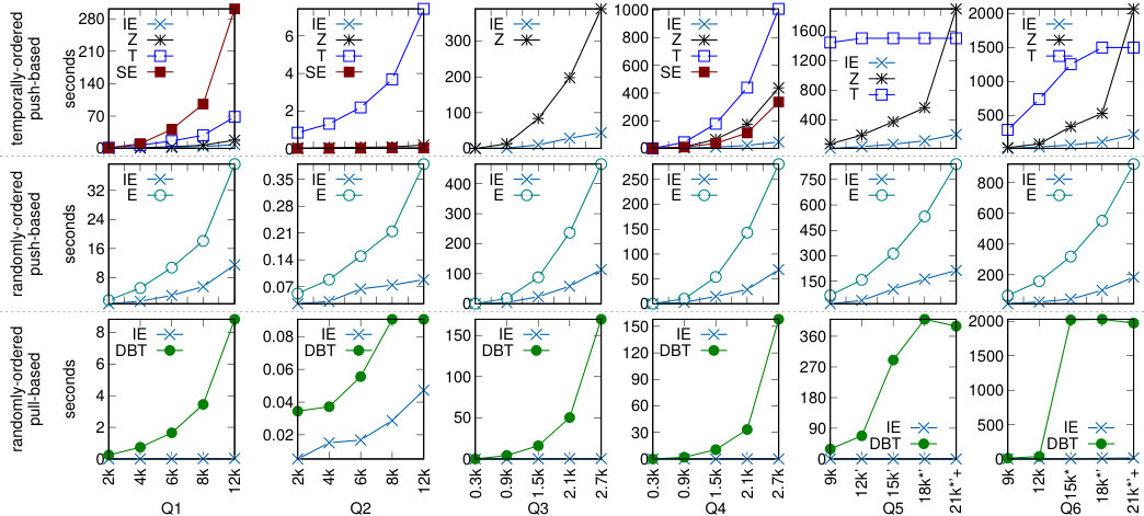 Figure 1
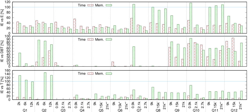 Figure 2
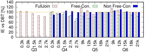 Figure 3
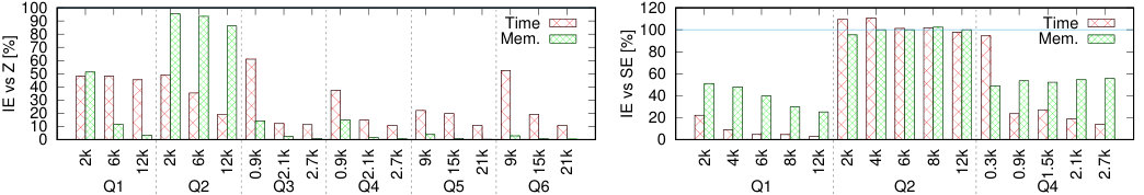 Figure 4
 Figure 5
 Figure 6
| Query | Expression |
|---|---|
| Query | ||
|---|---|---|
| 12k | 18,017k | |
| 12k | 3.8k | |
| 2.7k | 178,847k | |
| 2.7k | 90,425k | |
| 21k | 411,669k | |
| 21k | 297,873k | |
| 2.7k | 114,561k | |
| 21k | 411,669k | |
| 21k | 99,043k | |
| 2.7k | 114,561k | |
| 21k | 294,139k | |
| 21k | 297,873k |
Peer Reviews
No public reviews on file for this paper yet. If you reviewed it on a platform where reviews are public (OpenReview, ICLR, NeurIPS, ICML), you can paste yours below so the community can read it here.
Videos
No videos yet. Explain this paper in a talk, walkthrough, or lecture? Add one.
Taxonomy
TopicsAdvanced Database Systems and Queries · Data Management and Algorithms · Data Quality and Management
\WarningFilter
latexText page
11institutetext: M. Idris 22institutetext: Université Libre de Bruxelles, Belgium and TU Dresden, Germany
22email: [email protected] 33institutetext: M. Ugarte 44institutetext: Université Libre de Bruxelles, Belgium
44email: [email protected] 55institutetext: S. Vansummeren 66institutetext: Université Libre de Bruxelles, Belgium
66email: [email protected] 77institutetext: Hannes Voigt 88institutetext: neo4j, Germany
This work was done while the author was affiliated to TU Dresden, Germany
88email: [email protected] 99institutetext: Wolfgang Lehner 1010institutetext: TU Dresden, Germany
1010email: [email protected]
Conjunctive Queries with Theta Joins Under Updates
Muhammad Idris
Martín Ugarte
Stijn Vansummeren
Hannes Voigt
Wolfgang Lehner
(Received: date / Accepted: date)
Abstract
Modern application domains such as Composite Event Recognition (CER) and real-time Analytics require the ability to dynamically refresh query results under high update rates. Traditional approaches to this problem are based either on the materialization of subresults (to avoid their recomputation) or on the recomputation of subresults (to avoid the space overhead of materialization). Both techniques have recently been shown suboptimal: instead of materializing results and subresults, one can maintain a data structure that supports efficient maintenance under updates and can quickly enumerate the full query output, as well as the changes produced under single updates. Unfortunately, these data structures have been developed only for aggregate-join queries composed of equi-joins, limiting their applicability in domains such as CER where temporal joins are commonplace. In this paper, we present a new approach for dynamically evaluating queries with multi-way -joins under updates that is effective in avoiding both materialization and recomputation of results, while supporting a wide range of applications. To do this we generalize Dynamic Yannakakis, an algorithm for dynamically processing acyclic equi-join queries. In tandem, and of independent interest, we generalize the notions of acyclicity and free-connexity to arbitrary -joins and show how to compute corresponding join trees. We instantiate our framework to the case where -joins are only composed of equalities and inequalities () and experimentally compare our algorithm to state of the art CER systems as well as incremental view maintenance engines. Our approach performs consistently better than the competitor systems with up to two orders of magnitude improvements in both time and memory consumption.
1 Introduction
The ability to analyze dynamically changing data is a key requirement of many contemporary applications, usually associated with Big Data, that require such analysis in order to obtain timely insights and implement reactive and proactive measures. Example applications include Financial Systems cormode2007 , Industrial Control Systems groover2007 , Stream Processing Stonebraker:2005 , Composite Event Recognition (CER, also known as Complex Event Processing) buchmann:2009 ; cugola:2012 , and Business Intelligence (BI) sahay2008 . Generally, the analysis that needs to be kept up-to-date, or at least their basic elements, are specified in a query language. The main task is then to efficiently update the query results under frequent data updates.
In this paper, we focus on the problem of dynamic evaluation for queries that feature multi-way -joins in addition to standard equi-joins. To illustrate our setting, consider that we wish to detect potential credit card frauds. Credit card transactions have a timestamp (ts), account number (acc), and amount (amnt), among other attributes. A typical fraud pattern is that the criminal tests the credit card with a few small purchases to then make larger purchases (cf. DBLP:conf/debs/Schultz-MollerMP09 ). In this respect, we would like to dynamically evaluate the following query, assuming new transactions arrive in a streaming fashion and the pattern must be detected in less than 1 hour.
SELECT * FROM Trans S1, Trans S2, Trans L WHERE S1.ts < S2.ts AND S2.ts < L.ts AND L.ts < S1.ts + 1h AND S1.acc = S2.acc AND S2.acc = L.acc AND S1.amnt < 100 AND S2.amnt < 100 AND L.amnt > 400
Queries like this with inequality joins appear in both CER and BI scenarios. Traditional techniques to process these queries dynamically can be categorized in two approaches: relational and automaton-based. We next discuss both approaches, their strengths and drawbacks.
Relational
Relational approaches, such as DBLP:journals/vldb/KochAKNNLS14 ; DBLP:conf/sigmod/MeiM09 ; DBLP:books/sp/16/ArasuBBCDIMSW16 are based on a form of Incremental View Maintenance (IVM). To process a query over a database , IVM techniques materialize the output and evaluate delta queries. Upon update , delta queries use , and the materialized to compute the set of tuples to add/delete from in order to obtain . If is small w.r.t. , this is expected to be faster than recomputing from scratch. To further speed up dynamic query processing, we may materialize not only but also the result of some subqueries. This is known as Higher-Order IVM (HIVM for short) DBToaster2016 ; DBLP:journals/vldb/KochAKNNLS14 ; DBLP:conf/pods/Koch10 . Both IVM and HIVM have drawbacks, however. First, materialization of requires space, where denotes the size of . Therefore, when is large compared to , materializing quickly becomes impractical, especially for main-memory based systems. HIVM is even more affected by this problem because it not only materializes the result of but also the results to some subqueries. For example, in our fraud query HIVM would materialize the results of the following join in order to respond quickly to the arrival of a potential transaction :
[TABLE]
If we assume that there are small transactions in the time window, all of the same account, this materialization will take space. This becomes rapidly impractical when becomes large.
Automata
Automaton-based approaches (e.g., brenna07 ; DBLP:conf/sigmod/WuDR06 ; DBLP:journals/jss/CugolaM12 ; DBLP:conf/debs/CugolaM10 ; Sase2014 ; DBLP:conf/sigmod/AgrawalDGI08 ) are primarily employed in CER systems. In contrast to the relational approaches, they assume that the arrival order of event tuples corresponds to the timestamp order (i.e., there are no out-of-order events) and build an automaton to recognize the desired temporal patterns in the input stream. Broadly speaking, there are two automata-based recognition approaches. In the first approach, followed by DBLP:conf/sigmod/WuDR06 ; DBLP:conf/sigmod/AgrawalDGI08 , events are cached per state and once a final state is reached a search through the cached events is done to recognize the complex events. While it is no longer necessary to check the temporal constraints during the search, the additional constraints (in our example, and ) must still be verified. If the additional constraints are highly selective this approach creates an unnecessarily large update latency, given that each event triggering a transition to a final state may cause re-evaluation of a sub-join on the cached data, only to find few new output tuples.
In the second approach, followed by brenna07 ; Sase2014 ; DBLP:journals/jss/CugolaM12 ; DBLP:conf/debs/CugolaM10 , partial runs are materialized according to the automaton’s topology. For our example query, this means that, just like HIVM, the join ( ‣ 1) is materialized and maintained so it is available when a large amount transaction arrives. This approach hence shares with HIVM its high memory overhead and maintenance cost.
It has been recently shown that the drawbacks of these two approaches can be overcome by a rather simple idea dyn:2017 ; olteanu:fivm . Instead of fully materializing (potentially large) results and subresults, we can build a compact representation of the query result that supports efficient maintenance under updates. The representation is equipped with index structures so that, whenever necessary, we can generate the actual query result one tuple at a time, spending a limited amount of work to produce each new result tuple. This makes the generation performance-wise competitive with enumeration from a fully materialized (non-compact) output. In essence, we are hence separating dynamic query processing into two stages: (1) an update stage where we only maintain under updates the (small) information that is necessary to be able to efficiently generate the query result and (2) an enumeration stage where the query result is efficiently enumerated. Moreover, for single-tuple updates the representation also supports efficient enumeration of the changes to the query result. This is relevant for push-based query processing systems, where users do not ping the system for the complete current query answer, but instead ask to be notified of the changes to the query results when the database changes.
This idea was first presented by a subset of the authors in the Dynamic Yannakakis Algorithm (Dyn for short) dyn:2017 , an algorithm for efficiently processing acyclic aggregate-join queries. Dyn is worst-case optimal for two classes of queries, namely the q-hierarchical and free-connex acyclic conjunctive queries. A different approach named F-IVM, based on so-called factorized databases, was later developed to dynamically process aggregate-join queries that are not necessarily acyclic or need to support complex aggregates olteanu:fivm .
Unfortunately, both Dyn and F-IVM are only applicable to queries with equality joins, and as such they do not support analytical queries with other types of joins like the ones with inequalities or disequalities . Therefore, the current state of the art techniques for dynamically processing queries with joins beyond equality suffer either from a high update latency (if subresults are not materialized) or a high memory footprint (if subresults are materialized). In this paper, we overcome these problems by generalizing the Dynamic Yannakakis algorithm to conjunctive queries with arbitrary -joins. We show that, in the specific case of inequality joins, this generalization performs consistently better than the state of the art, with up to two orders of magnitude improvements in processing time and memory consumption.
Contributions
We focus on the class of Generalized Conjunctive Queries (GCQs for short), which are conjunctive queries with -joins, that are evaluated under multiset semantics.
(1) We devise a succinct and efficiently updatable data structure to dynamically process GCQs. To this end, we first generalize the notions of acyclicity and free-connexity to queries with arbitrary -joins (Section 3). Our data structure degrades gracefully: if a GCQ only contains equalities our approach inherits the worst-case optimality provided by Dyn.
(2) We present GDyn, a general framework for extending Dyn to free-connex acyclic GCQs. Our treatment is general in the sense that the -join predicates are treated abstractly. GDyn hence applies to all predicates, not only inequality joins. We analyze the complexity of GDyn, and identify properties of indexing structures that are required in order for GDyn to support efficient enumeration of results as well as efficient update processing (Section 5).
(3) We instantiate GDyn to the particular case of inequality and equality joins. We show that updates can be processed in time , where is the size of the database plus the size of the update, and results can be enumerated with logarithmic delay. Moreover, if there is at most one inequality between any pair of relations, updates take time and enumeration is with constant delay. We call the resulting algorithm IEDyn. We first illustrate this algorithm by means of an extensive example (Section 4), and then describe the required data structures formally at the end of Section 5.
(4) The operation of GDyn and IEDyn is driven by a Generalized Join Tree (GJT). GJTs are essentially query plans that specify the data structure to be materialized, how it should be updated, and how to enumerate the query results. We present an algorithm that can be used both to check whether a GCQ is (free-connex) acyclic and to construct a corresponding GJT if this is the case. (Section 6).
(5) We experimentally compare IEDyn with state-of-the-art HIVM and CER frameworks. IEDyn performs consistently better, with up to two order of magnitude improvements in both speed and memory consumption (Section 7 and Section 8).
We introduce the required background in Section 2.
Additional material
This article presents the following additional contributions compared to its previously published conference version DBLP:journals/pvldb/IdrisUVVL18 :
(1) Correctness proofs. The conference version only sketched why GDyn and IEDyn work correctly and within the claimed bounds. In contrast, here we formally prove correctness.
(2) Novel algorithm for computing GJTs. As outlined, above, GDyn and IEDyn work on acyclic GCQs and their operation is driven by the specification of a GJT for such queries. The conference version only stated that an algorithm for checking acyclicity and free-connexity and computing GJTs exists. In contrast, here, we fully present this algorithm and illustrate its correctness.
Additional related work
In addition to the work already cited on CER and (H)IVM, our setting is closely related to query evaluation with constant delay enumeration Bagan:2007 ; DBLP:journals/sigmod/Segoufin15 ; Berkholz:2017 ; braultbaron ; Olteanu:2015 ; Bakibayev:2013 ; Olteanu:2015 ; Schleich:2016 ; dyn:2017 ; olteanu:fivm . This setting, however, deals with equi-joins only. Also related, although restricted to the static setting, is the practical evaluation of binary DBLP:conf/vldb/DeWittNS91 ; DBLP:conf/vldb/HellersteinNP95 ; DBLP:conf/sigmod/EnderleHS04 and multi-way DBLP:journals/is/BernsteinG81 ; DBLP:conf/vldb/YoshikawaK84 inequality joins. Our work, in contrast, considers dynamic processing of multi-way -joins, with a specialization to inequality joins. Recently, Khayyat et al. DBLP:journals/vldb/KhayyatLSOPQ0K17 proposed fast multi-way inequality join algorithms based on sorted arrays and space efficient bit-arrays. They focus on the case where there are exactly two inequality conditions per pairwise join. While they also present an incremental algorithm for pairwise joins, their algorithm makes no effort to minimize the update cost in the case of multi-way joins. As a result, they either materialize subresults (implying a space overhead that can be more than linear), or recompute subresults. We do neither.
2 Preliminaries
Traditional conjunctive queries are cross products between relations, restricted by equalities. Similarly, generalized conjunctive queries (GCQs) are cross products between relations, but restricted by arbitrary predicates. We use the following notation for queries.
Query Language
Throughout the paper, let denote variables (also commonly called column names or attributes). A hyperedge is a finite set of variables. We use , …to denote hyperedges. A GCQ is an expression of the form
[TABLE]
Here are relation symbols; are hyperedges (of the same arity as ); are predicates over , respectively; and both and are subsets of . We treat predicates abstractly: for our purpose, a predicate over is a (not necessarily finite) decidable set of tuples over . For example, is the set of all tuples satisfying . We indicate that is a predicate over by writing . Throughout the paper, we consider only non-nullary predicates, i.e., predicates with .
Example 1.
The following query is a GCQ.
[TABLE]
Intuitively, the query asks for the natural join between , , and , and from this result select only those tuples that satisfy both and .
We call the output variables of and denote it by . If then is called a full query and we may omit the symbol altogether for brevity. The elements are called atomic queries (or atoms). We write for the set of all atoms in , and for the set of all predicates in . A normal conjunctive query (CQ for short) is a GCQ where .
Semantics
We evaluate GCQs over Generalized Multiset Relations (GMRs for short) DBLP:journals/vldb/KochAKNNLS14 ; DBLP:conf/pods/Koch10 ; dyn:2017 . A GMR over is a relation over (i.e., a finite set of tuples with schema ) in which each tuple is associated with a non-zero integer multiplicity .111In their full generality, GMRs can carry multiplicities that are taken from an arbitrary algebraic ring structure (cf., DBLP:conf/pods/Koch10 ), which can be useful to describe the computation of aggregations over the result of a GCQ. To keep the notation and discussion simple, we fix the ring of integers throughout the paper but our result generalize trivially to arbitrary rings. In contrast to classical multisets, the multiplicity of a tuple in a GMR can hence be negative, allowing to treat insertions and deletions uniformly. We write for the finite set of all tuples in ; to indicate ; and for . A GMR is positive if for all .
The operations of GMR union (), minus , projection (), natural join () and selection () are defined similarly as in relational algebra with multiset semantics. Figure 1 illustrates these operations. We refer to dyn:2017 ; DBLP:journals/vldb/KochAKNNLS14 for a formal semantics. We abbreviate by and, if , we abbreviate by .
A database over a set of atoms is a function that maps every atom to a positive GMR over . Given a database over the atoms occurring in query , the evaluation of over , denoted , is the GMR over constructed in the expected way: take the natural join of all GMRs in the database, do a selection over the result w.r.t. each predicate, and finally project on .
Updates and deltas
An update to a GMR is simply a GMR over the same variables as . Applying update to yields the GMR . An update to a database is a collection of (not necessarily positive) GMRs, one GMR for every atom of , such that is positive. We write for the database obtained by applying to each atom of , i.e., , for every atom of . For every query , every database and every update to , we define the delta query of w.r.t. and by . As such, is the update that we need to apply to in order to obtain .
Enumeration with bounded delay
A data structure supports enumeration of a set if there is a routine such that outputs each element of exactly once. Such enumeration occurs with delay if the time until the first output; the time between any two consecutive outputs; and the time between the last output and the termination of , are all bounded by . supports enumeration of a GMR if it supports enumeration of the set . When evaluating a GCQ , we will be interested in representing the possible outputs of by means of a family of data structures, one data structure for each possible input database . We say that can be enumerated from with delay , if for every input we can enumerate from with delay , where assigns a natural number to each . Intuitively measures in some way. In particular, if is constant we say the results are generated from the data structure with constant-delay enumeration (CDE).
As a trivial example of CDE of a GMR , assume that the pairs of are stored in an array (without duplicates). Then supports CDE of : simply iterates over each element in , one by one, always outputting the current element. Since array indexation is a operation, this gives constant delay. This example shows that CDE of the result of a query on input database , can always be done naively by materializing in an in-memory array . Unfortunately, then requires memory proportional to which, depending on , can be of size polynomial in . We hence search for other data structures that can represent using less space, while still allowing for efficient enumeration. Our experiments in Section 7 show that for the data structures described in this paper, CDE is indeed competitive with enumeration from an array while requiring much less space.
Computational Model
It is important to note that we focus on dynamic query evaluation in main memory. Furthermore, we assume a model of computation where the space used by tuple values and integers, the time of arithmetic operations on integers, and the time of memory lookups are all . We also assume that every GMR can be represented by a data structure that allows (1) enumeration of with constant delay; (2) multiplicity lookups in time given ; (3) single-tuple insertions and deletions in time; while (4) having a size that is proportional to the number of tuples in the support of . Essentially, our assumptions amount to perfect hashing of linear size cormen2009introduction . Although this is not realistic for practical computers Papadimitriou:2003 , it is well known that complexity results for this model can be translated, through amortized analysis, to average complexity in real-life implementations cormen2009introduction .
3 Generalized Acyclicity
Join queries are GCQs without projections that feature equality joins only. The well-known subclass of acyclic join queries abiteboul1995foundations ; DBLP:conf/vldb/Yannakakis81 , in contrast to the entire class of join queries, can be evaluated in time , i.e., linear in both input and output. This result relies on the fact that acyclic join queries admit a tree structure that can be exploited during evaluation. In previous work dyn:2017 , we showed that this tree structure can also be exploited for efficient processing of CQs under updates. In this section, we therefore extend the tree structure and the notion of acyclicity from join queries to GCQs with both projections and arbitrary -joins. We begin by defining this tree structure and the related notion of acyclicity for full GCQs. Then, we proceed with the notion corresponding to GCQs that feature projections, known as free-connex acyclicity.
Generalized Join Trees
To simplify notation, we denote the set of all variables (resp. atoms, resp. predicates) that occur in an object (such as a query) by (resp. , resp. ). In particular, if is itself a set of variables, then . We extend this notion uniformly to labeled trees. E.g., if is a node in tree , then denotes the set of variables occurring in the label of , and similarly for edges and trees themselves. Finally, we write for the set of children of in tree . If is clear from the context, we omit subscripts from our notation.
Definition 1 (GJT).
A Generalized Join Tree (GJT) is a node-labeled and edge-labeled directed tree such that:
- •
Every leaf is labeled by an atom.
- •
Every interior node is labeled by a hyperedge and has at least one child such that .
- •
Whenever the same variable occurs in the label of two nodes and of , then occurs in the label of each node on the unique path linking and . This condition is called the connectedness condition.
- •
Every edge from parent to child in is labeled by a set of predicates. It is required that for every predicate we have .
Let be a node in GJT . Every node with is called a guard of . Observe that every interior node must have a guard child by the second requirement above. Since this child must itself have a guard child, which must itself have a guard child, and so on, it holds that every interior node has at least one guard descendant that is a leaf.
Definition 2.
A GJT is a GJT for GCQ if and the number of times that an atom occurs in equals the number of times that it occurs as a label in , and . A GCQ is acyclic if there is a GJT for . It is cyclic otherwise.
Example 2.
The two trees depicted in Fig. 2 are GJTs for the following full GCQ , which is hence acyclic.
[TABLE]
In contrast, the query (also known as the triangle query) is the prototypical cyclic join query.
If does not contain any predicates, that is, if is a CQ, then the last condition of Definition 1 vacuously holds. In that case, the definition corresponds to the definition of a generalized join tree given in dyn:2017 , where it was also shown that a CQ is acyclic under any of the traditional definitions of acyclicity (e.g., abiteboul1995foundations ) if and only if the query has a GJT for with . In this sense, Definition 2 indeed generalizes acyclicity from CQs to GCQs.
Discussion
The notion of ayclicity for normal CQs is well-studied in database theory abiteboul1995foundations and has many equivalent definitions, including a definition based on the existence of a full reducer. Here, a full reducer for a CQ is a program in the semijoin algebra (the variant of relational algebra where joins are replaced by semijoins) that, given a database computes a new database with the following properties. (1) ; (2) for every atom ; and (3) no strict subset of has . In other words, selects a minimal subset of needed to answer .
Bernstein and Goodman DBLP:journals/is/BernsteinG81 consider conjunctive queries with inequalities and classify the class of such queries that admit full reducers. As such, one can view this as a definition of acyclicity for conjunctive queries with inequalities. Bernstein and Goodman’s notion of acyclicity is incomparable to ours. On the on hand, our definition is more general: Bernstein and Goodman consider only queries where for each pair of atoms there is exactly one variable being compared by means of equality or inequality. We, in contrast, allow an arbitrary number of variables to be compared per pair of atoms. In particular, Bernstein and Goodman’s disallow queries like since it compares with by means of equality and by means of inequality, while this is trivially acyclic in our setting.
On the other hand, for this more restricted class of queries, Bernstein and Goodman show that certain queries that we consider to be cyclic have full reducers (and would be hence acyclic under their notion). An example here is
[TABLE]
The crucial reason that this query admits a full reducer is due to the transitivity of . Since our notion of acyclicity interprets predicates abstractly and does hence not assume properties such as transitivity on them, we must declare this query cyclic (as can be checked by running the algorithm of Section 6 on it). It is an interesting direction for future work to incorporate Bernstein and Goodman’s notion of acyclicity in our framework.
Free-connex acyclicity
Acyclicity is actually a notion for full GCQs. Indeed, note that whether or not is acyclic does not depend on the projections of (if any). To also process queries with projections efficiently, a related structural constraint known as free-connex acyclicity is required.
Definition 3 (Connex, Frontier).
Let be a GJT. A connex subset of is a set that includes the root of such that the subgraph of induced by is a tree. The frontier of a connex set is the subset consisting of those nodes in that are leaves in the subtree of induced by .
To illustrate, the set is a connex subset of the tree shown in Fig. 2. Its frontier is . In contrast, is not a connex subset of .
Definition 4 (Compatible, Free-Connex Acyclic).
A GJT pair is a pair with a GJT and a connex subset of . A GCQ is compatible with if is a GJT for and . A GCQ is free-connex acyclic if it has a compatible GJT pair.
In particular, every full acyclic GCQ is free-connex acyclic since the entire set of nodes of a GJT for is a connex set with . Therefore, is a compatible GJT pair for .
Example 3.
Let with the GCQ from Example 2. is free-connex acyclic since it is compatible with the pair with the GJT from Fig. 2. By contrast, is not compatible with any GJT pair containing , since any connex set of that includes a node with variable will also include variable , which is not in . Finally, it can be verified that no GJT pair is compatible with ; this query is hence not free-connex acyclic.
In Section 6 we show how to efficiently check free-connex acyclicity and compute compatible GJT pairs.
Binary GJTs and sibling-closed connex sets
As we will see in Sections 4 and 5, a GJT pair essentially acts as query plan by which GDyn and IEDyn process queries dynamically. In particular, the GJT specifies the data structure to be maintained and drives the processing of updates, while the connex set drives the enumeration of query results.
In order to simplify the presentation of what follows, we will focus exclusively on the class of GJT pairs with a binary GJT and sibling-closed.
Definition 5 (Binary, Sibling-closed).
A GJT is binary if every node in it has at most two children. A connex subset of is sibling-closed if for every node with a sibling in , is also in .
Our interest in limiting to sibling-closed connex sets is due to the following property, which will prove useful for enumerating query results, as explained in Section 4.
Lemma 1.
If is a sibling-closed connex subset, then where is the frontier of .
Proof.
Since the inclusion is immediate. It remains to prove . To this end, let be an arbitrary but fixed node in . We prove that by induction on the height of in , which is defined as the length of the shortest path from to a frontier node in . The base case is where the height is zero, i.e., , in which case trivially holds. For the induction step, assume that the height of is . In particular, is not a frontier node, and has at least one child in . Because is sibling-closed, all children of are in . In particular, the guard child of is in and has height at most . By induction hypothesis, . Then, because is a guard of , , as desired. ∎
Let us call a GJT pair binary if is binary, and sibling-closed if is sibling-closed. We say that two GJT pairs and are equivalent if and are equivalent and . Two GJTs and are equivalent if , the number of times that an atom appears as a label in equals the number of times that it appears in , and .
The following proposition shows that we can always convert an arbitrary GJT pair into an equivalent one that is binary and sibling-closed. As such, we are assured that our focus on binary and sibling-closed GJT pairs is without loss of generality.
Proposition 1.
Every GJT pair can be transformed in polynomial time into an equivalent pair that is binary and sibling closed.
The rest of this section is devoted to proving Proposition 1. We do so in two steps. First, we show that any pair can be transformed in polynomial time into an equivalent sibling-closed pair. Next, we show that any sibling-closed GJT pair can be converted in polynomial time into an equivalent binary and sibling-closed pair. Proposition 1 hence follows by composing these two transformations.
Sibling-closed transformation
We say that is a violator node in a GJT pair if and some, but not all children of are in . A violator is of type 1 if some node in is a guard of . It is of type 2 otherwise. We now define two operations on that remove violators of type 1 and type 2, respectively. The sibling-closed transformation is then obtained by repeatedly applying these operators until all violators are removed.
The first operator is applicable when is a type 1 violator. It returns the pair obtained as follows:
- •
Since is a type 1 violator, some is a child guard of (i.e., ).
- •
Because every node has a guard, there is some leaf node that is a descendant guard of (i.e. ). Possibly, is itself.
- •
Now create a new node between node and its parent with label . Since is a descendant guard of and , becomes a descendant guard of and as well. Detach all nodes in from and attach them as children to , preserving their edge labels. This effectively moves all subtrees rooted at nodes in from to . Denote by the final result.
- •
If was not in , then . Otherwise, .
We write to indicate that can be obtained by applying the above-described operation on node .
Example 4.
Consider the GJT pair from Fig. 3 where is indicated by the nodes in the shaded area. Let us denote the root node by and its guard child with label by . The node is a descendant guard of . Since is not in , is violator of type
- After applying the operation 1 for the choice of guard node and descendant guard node , shows the resulting valid sibling-closed GJT.
Lemma 2 ().
Let be a violator of type in and assume . Then is a GJT pair and it is equivalent to . Moreover, the number of violators in is strictly smaller than the number of violators in .
We prove this lemma in Appendix A. The second operator is applicable when is a type 2 violator. When applied to in it returns the pair obtained as follows:
- •
Since is a type 2 violator, no node in is a guard of . Since every node has a guard, there is some which is a guard of .
- •
Create a new child of with label ; detach all nodes in (including ) from , and add them as children of , preserving their edge labels. This moves all subtrees rooted at nodes in from to . Denote by the final result.
- •
Set .
We write to indicate that was obtained by applying this operation on .
Example 5.
Consider the GJT pair in Fig. 4. Let us denote the root node by . Since its guard child is not in , is violator of type 2. After applying operation 2 on , shows the resulting valid sibling-closed GJT.
Lemma 3 ().
Let be a violator of type in and assume . Then is a GJT pair and it is equivalent to . Moreover, the number of violators in is strictly smaller than the number of violators in .
The proof can be found in Appendix A.
Proposition 2.
Every GJT pair can be transformed in polynomial time into an equivalent sibling-closed pair.
Proof.
The two operations introduced above remove violators, one at a time. By repeatedly applying these operations until no violator remains we obtain an equivalent pair without violators, which must hence be sibling-closed. Since each operator can clearly be executed in polynomial time and the number of times that we must apply an operator is bounded by the number of nodes in the GJT pair, the removal takes polynomial time. ∎
Binary transformation
Next, we show how to transform a sibling-closed pair into an equivalent binary and sibling-closed pair . The idea here is to “binarize” each node with children as shown in Fig. 5. There, we assume without loss of generality that is a guard child of . The binarization introduces new intermediate nodes , all with . Note that, since is a guard of and , it is straightforward to see that will be a guard of , which will be a guard of , which will be a guard of , and so on. Finally, will be a guard of . The connex set is updated as follows. If none of ’s children are in i.e. is a frontier node, set . Otherwise, since is sibling-closed, all children of are in , and we set . Clearly, remains a sibling-closed connex subset of and . We may hence conclude:
Lemma 4.
By binarizing a single node in a sibling-closed GJT pair as shown in Fig. 5, we obtain an equivalent GJT pair that has strictly fewer non-binary nodes than .
Binarizing a single node is a polynomial-time operation. Then, by iteratively binarizing non-binary nodes until all nodes have become binary we hence obtain:
Proposition 3.
Every sibling-closed GJT pair can be transformed in polynomial time into an equivalent, binary and sibling-closed pair.
4 Dynamic joins with equalities and inequalities: an example
In this section we illustrate how to dynamically process free-connex acyclic GCQs when all predicates are inequalities . We do so by means of an extensive example that shows the indexing structures and GMRs. The definitions and algorithms (that apply to arbitrary -joins) will be formally presented in Section 5.
Throughout this section we consider the following query , which is free-connex acyclic (see Example 3):
[TABLE]
Let be the GJT from Fig. 2. We process based on a -reduct, a data structure that succinctly represents the output of . For every node , define as the set of all predicates on outgoing edges of , i.e.
Definition 6 (-reduct).
Let be a GJT for a query and let be a database over . The -reduct (or semi-join reduction) of is a collection of GMRs, one GMR for each node , defined inductively as follows:
if is an atom, then
- -
if has a single child , then
- -
otherwise, has two children and . In this case we have .
Fig. 6 depicts an example database (top) and its -reduct (bottom). Note, for example, that the only tuple in the GMR at the root is the join of and restricted to and projected over .
It is important to observe that the size of a -reduct of a database can be at most linear in the size of . The reason is that, as illustrated in Fig. 6, for each node there is some descendant atom (possibly itself) such that . Note that , in contrast, can easily become polynomial in the size of in the worst case.
Enumeration
From a -reduct we can enumerate the result rather naively simply by recomputing the query results, in particular because we have access to the complete database in the leaves of . We would like, however, to make the enumeration as efficient as possible. To this end, we equip -reducts with a set of indices. To avoid the space cost of materialization, we do not want the indices to use more space than the -reduct itself (i.e., linear in ). We illustrate these ideas in our running example by introducing a simple set of indices that allow for efficient enumeration.
Let be the connex subset of satisfying . is compatible with , binary and sibling-closed. We rely on the sibling-closed property of to enumerate query results, and can do so without loss of generality by Proposition 1. To enumerate the query results, we will traverse top-down the nodes in . The traversal works as follows: for each tuple in , we consider all tuples in that are compatible with , and all tuples that are compatible with . Compatibility here means that the corresponding equalities and inequalities are satisfied. Then, for each pair , we output the tuple with multiplicity . A crucial difference here with naive recomputation is that, since is already a join between and , we will only iterate over relevant tuples: each tuple that we iterate over will produce a new output tuple. For example, we will never look at the tuple in because it does not have a compatible tuple at the root.
To implement this enumeration strategy efficiently, we desire index structures on and that allow to enumerate, for a given tuple in , all compatible tuples (resp. ) with constant delay. In the case of this is achieved simply by keeping sorted decreasingly on variable . Given tuple , we can enumerate the compatible tuples from by iterating over its tuples one by one in a decreasing manner, starting from the largest value of , and stopping whenever the current value is smaller or equal than the value in . For indexing we use a more standard index. Since we need to enumerate all tuples that have the same and value as , CDE can be achieved by using a hash-based index on and . This index is depicted as in Fig. 7. We can see that, since the described indices provide CDE of the compatible tuples given , our strategy provides enumeration of with constant delay if we assume the query to be fixed (i.e. in data complexity Vardi:1982 ).
Updates
Next we illustrate how to process updates. The objective here is to transform the -reduct of into a -reduct of , where is the received update. To do this efficiently we use additional indexes on . We present the intuitions behind these indices with an update consisting of two insertions: with multiplicity and with multiplicity . Fig. 7 depicts the update process highlighting the modifications caused by the update.
Let us first discuss how to process the tuple . We proceed bottom-up, starting at which is itself affected by the insertion of . Subsequently, we need to propagate the modification of to its ancestors and . Concretely, from the definition of -reduction, it follows that we need to add some modifications to , , and on :
- ,
- ,
- .
To compute the joins on the right-hand sides efficiently, we create a number of additional indexes on , and . Concretely, in order to efficiently compute , we group tuples in the GMR by the variables that has in common with (in this case ) and then, per group, sort tuples ascending on variable . We mark grouping variables in Fig. 7 with (e.g. ), and sorting by (for ascending, e.g., ) and (for descending). A hash index on the grouping variables (denoted in Fig. 7) then allows to find the group given a value. The join can then be processed by means of a hybrid form of sort-merge and index nested loop join. Sort ascendingly on and . For each -group in find the corresponding group in by passing the value to the index . Let be the first tuple in the group. Then iterate over the tuples of the group in the given order and sum up their multiplicities until becomes larger than . Add to the result with its original multiplicity multiplied by the found sum (provided it is non-zero). Then consider the next tuple in the group, and continue summing from the current tuple in the group until becomes again larger than , and add the result tuple with the correct multiplicity. Continue repeating this process for each tuple in the group, and for each group in . In our case, there is only one group in (given by ) and we will only iterate over the tuple in , obtaining a total multiplicity of 2, and therefore compute . In order to compute the join efficiently, we proceed similarly. Here, however, there are no grouping variables on and it hence suffices to sort descendingly on . Note that this was actually already required for efficient enumeration. Also note that is empty.
Now we discuss how to process . First, we insert into . We need to propagate this change to the parent by calculating . This is done by a simple hash-based aggregation. Finally, we need to propagate to the root by computing . To process this join efficiently we proceed as before. Again, there are no grouping variable on (since it has no variables in common with ) and it hence suffices to sort ascending on . The only tuple that we iterate over during the hybrid join is wich has multiplicity 12. Hence, we have , concluding the example.
5 Dynamic Yannakakis Over GCQs
Dynamic Yannakakis (Dyn) is an algorithm to efficiently evaluate free-connex acyclic aggregate-equijoin queries under updates dyn:2017 . This algorithm matches two important theoretical lower bounds (for q-hierarchical CQs Berkholz:2017 and free-connex acyclic CQs Bagan:2007 ), and is highly efficient in practice. In this section we present a generalization of Dyn, called GDyn, to dynamically process free-connex acyclic GCQs. Since predicates in a GCQ can be arbitrary, our approach is purely algorithmic; the efficiency by which GDyn process updates and produces results will depend entirely on the efficiency of the underlying data structures. Here we only describe the properties that those data structures should satisfy and present the general (worst-case) complexity of the algorithm. The techniques and indices presented in the previous section provide a practical instantiation of GDyn to a GCQ with equalities and inequalities, and throughout this section we make a parallel between that instantiation and the more abstract definitions of GDyn.
In this section we assume that is a free-connex acyclic GCQ and that is a binary and sibling-closed GJT pair compatible with . Like in the case of equalities and inequalities, the dynamic processing of will be based on a -reduct of the current database . A set of indices will be added to optimize the enumeration of query results and maintenance of the -reduct under updates. We formalize the notion of index as follows:
Definition 7 (Index).
Let be a GMR over , let be a hyperedge, let be a hyperedge satisfying , and let be a predicate with . An index on by with delay is a data structure that provides, for any given GMR over , enumeration of with delay . The update time of index is the time required to update to an index on (by ) given update to .
For example, in Fig. 7 is used as an index on by . Indeed, in the previous section we precisely discussed how allows to efficiently compute for an update to . Having the notion of index, we discuss how GDyn enumerates query results and processes updates.
Enumeration
Let be the current database. To enumerate from a -reduct of we can iterate over the reductions with in a nested fashion, starting at the root and proceeding top-down. When is the root, we iterate over all tuples in . For every such tuple , we iterate only over the tuples in the children of that are compatible with (i.e., tuples in that join with and satisfy ). This procedure continues until we reach nodes in the frontier of at which time the output tuple can be constructed. The pseudocode is given in Algorithm 1, where the tuples that are compatible with are computed by .
Now we show the correctness of the enumeration algorithm, for which we need to introduce some further notation. Let , and be as above. Given a node we denote the sub-tree of rooted at by , and define the query induced by as
[TABLE]
where and are the sets of all atoms and predicates occurring in , respectively.
Lemma 5 ().
Let , , , and be defined as above, and let be a -reduct for . Then, .
The proof by induction is detailed in Appendix B. To show correctness of enumeration, we need the following additional lemma regarding the subroutine of Algorithm 1 (Line 3). The proof is again by induction and detailed in Appendix B.
Lemma 6 ().
Let , , and be as above. If is a -reduct of , then for every node and every tuple in , correctly enumerates .
Proposition 4.
Let , , and be as above. Then enumerates .
Proof.
Let be the root of . By Lemma 5 we have , and therefore is a projection of . This implies that , which is equivalent to the disjoint union . By Lemma 6, it is clear that this is exactly what enumerates. ∎
We now analyze the complexity of . First, observe that by definition of -reducts, compatible tuples will exist at every node. Hence, every tuple that we iterate over will eventually produce a new output tuple. This ensures that we do not risk wasting time in iterating over tuples that in the end yield no output. As such, the time needed for to produce a single new tuple is determined by the time taken to enumerate the tuples in , where is the parent of . Since this is equivalent to we can do this efficiently by creating an index on by . For example, in Section 4 we defined hash-maps and group-sorted GMRs so that given one tuple from a parent we could enumerate the compatible tuples in the child with constant delay. In general, the efficiency of enumeration will depend on the delay provided by the indices.
Proposition 5.
Assume that for every we have an index on by with delay , where is the parent of and is a monotone function. Then, using these indices, correctly enumerates with delay where is given by . Thus, the total time required to execute is .
Proof.
We show that for every and , the call enumerates with delay . We proceed by induction in . If then and the delay is clearly constant as the algorithm will only yield . Now assume that . If has a single child , the index on by allows us to iterate over with delay and therefore delay . For each element of this enumeration, the algorithm calls , which by induction hypothesis enumerates with delay . Then, the maximum delay between two outputs is , and since this is in
[TABLE]
The final observation is that the sets are disjoint for different values of , and thus the enumeration does not produce repeated values.
For the case in which has two children and , by similar reasoning it is easy to show that the maximum delay between two outputs is
[TABLE]
[TABLE]
[TABLE]
It is also important to mention that the sets enumerated by are disjoint for each (), and that for each and , it is the case that and are compatible, thus producing outputs in every iteration. ∎
In particular, if is constant we enumerate with delay (i.e. constant in data complexity).
Update processing
To allow enumeration of under updates to we need to maintain the -reduct (and, if present, its indexes) up to date. As illustrated in the previous section, it suffices to traverse the nodes of in a bottom-up fashion. At each node we have to compute the delta of . For leaf nodes, this delta is given by the update itself. For interior nodes, the delta can be computed from the delta and original reduct of its children. Algorithm 2 gives the pseudocode.
The fundamental part of Algorithm 2 is to compute joins and produce delta GMRs (Line 10), propagating updates from each node to its parent. When there is an update to a node with sibling and parent , we need to compute . To do this efficiently, we naturally store an index on by . For example, we discussed how the hash-map in Fig. 7 plus the sorting on of allowed us to efficiently compute .
Summarizing, to efficiently enumerate query results and process updates we need to store a -reduct plus a set of indices on its GMRs. The data structure containing these elements is called a -representation.
Definition 8 (-representation).
Let be a database. A -representation (-rep for short) of is composed by a -reduct of and, for each node with parent , the following set of indices:
If belongs to , then we store an index on by .
- -
If is a node with a sibling , then we store an index on by .
Together with the notion of -rep, Algorithms 1 and 2 provide a framework for dynamic query evaluation. By constructing the -reduct and set of indices (and their update procedures) one can process free-connex acyclic GCQs under updates. Naturally, to implement such framework one needs to devise indices for a particular set of predicates. For example, Dyn is an instantiation to the class of CQs, and in the previous section we showed how to instantiate this framework for a GCQ based on equalities and inequalities. Next, we present the general set of indices required to process free-connex acyclic GCQs with equalities and inequalities.
IEDyn
For queries that have only inequality predicates, the instantiation of a -representation of contains a -reduct of and, for each node with parent , the following data structures:
If , the index on from Definition 8 is obtained by doing two things. (1) First, group according to the variables in . Then, per group, sort the tuples according to the variables of mentioned in (if any). (2) Create a hash table that maps each tuple to its corresponding group in . If is empty this hash table is omitted.
- -
If has a sibling , the index of Definition 8 is obtained by doing two things. (1) First, group according to the variables in . Then, per group, sort the tuples according to the variables of mentioned in (if any). (2) Create a hash table mapping each to the corresponding group in . If is empty this hash table is omitted.
In Wection 4 we illustrated how use these data structures. Effectively, in Figure 7 and are examples of , used for update propagation, while is an example of , used for enumeration.
Note that the example query from Section 4 has at most one inequality between each pair of atoms. This causes each edge in to consist of at most inequality. As such, when creating the index for a node , the reduct will be sorted per group according to at most one variable. This is important for enumeration delay because, as exemplified in Section 4, we can then find compatible tuples by first the corresponding group and then iterating over the sorted group from the start and stopping when the first non-compatible tuple is found. When there are multiple inequalities per pair of atoms then we will need to sort according to multiple variables under some lexicographic order. This causes enumeration delay to become logarithmic since then compatible tuples will intermingle with non-compatible tuples, and a binary search is necessary to find the next batch of compatible tuples in the group.
We call IEDyn the algorithm for processing free-connex acyclic GCQs with equalities and inequalities.
Theorem 5.1.
Let be a GCQ in which all predicates are equalities and inequalities. Let be a binary and sibling-closed GJT pair compatible with . Given a database over , a -rep of , under IEDyn Algorithm 1 enumerates with delay . Also, given an update under IEDyn Algorithm 2 transforms into a -rep of in time , where .
Proof.
Let us first prove the enumeration bounds. It is immediate to see that for every node the GMR satisfies , given that is defined as a series of semi-joins based on (or, equivalently, because every internal node has a guard). Therefore, according to Proposition 5 the enumeration delay is where is the connex subset of and is the delay provided by the index . Now, from the description of IEDyn these indices are implemented as hash tables that map each tuple in to a lexicographically sorted set containing , where is a parent-child pair. Therefore, given a tuple we can enumerate by first projecting over and then iterating over all tuples satisfying . Since these predicates are only inequalities, each group can be kept sorted lexicographically and, as mentioned earlier, enumeration can be achieved with logarithmic delay. It follows from Prop. 5 that the enumeration delay is .
Now we discuss update time. As can be seen in Algorithm 2, for each parent-child pair we need to compute either or , depending on whether or not has a sibling . If does not have a sibling, computing can be done directly by sorting lexicographically, enumerating those tuples satisfying (with logarithmic delay), and finally projecting over . This takes time in , which is clearly contained in since . The more involved case is when has a sibling and we need to compute . Here we first sort lexicographically. Then, for every tuple in compute . Note that this can be done in time since from the constructed data structures we can enumerate with logarithmic delay. Because the previous procedure needs to be performed for each , this can be done in time and therefore in time . Note that here we ignore the sorting steps as well as the maintenance of the corresponding GMRs as those steps are clearly . Finally, since we need to perform the procedure described above once per each parent-child pair, the entire routine takes at most ). ∎
From the previous result we can see that for the general case of equalities and inequalities we already have a procedure that can be quadratic in the size of the database.222In the conference version of this paper DBLP:journals/pvldb/IdrisUVVL18 there was an incorrect claim: we stated that updates could be processed in time in data complexity. We then found a bug in our algorithm and we currently do not know if this bound can be achieved. However, if we restrict the use of inequalities in a particular way, we can speed up both update processing and enumeration delay.
Theorem 5.2.
Let , and be defined as in Theorem 5.1, and assume that for each it is the case that . Given a database over , a -rep of , under IEDyn Algorithm 1 enumerates with delay . Also, given an update under IEDyn Algorithm 2 transforms into a -rep of in time , where .
Proof.
The main observation to prove this result is that when there is a single predicate, a lexicographically sorted set is totally sorted by a single attribute. Regarding enumeration, this implies that given a parent-child pair and a tuple , we can enumerate with constant delay. The reason behind this is that the index maps to a totally sorted set, and therefore we can start from the largest/smallest value of the relevant attribute, and iterate over all tuples decreasingly/increasingly until we find a tuple that does not satisfy the inequality. At that point we are certain that we have visited all tuples satisfying the inequality.
The update processing can also be improved by a similar argument, although the modification is slightly more involved. Assume again that we have a parent-child pair and want to compute , where is the sibling of . We do so efficiently as follows. Recall that the index groups by and sorts each group by the variables involved in . We construct an index over with the same characteristics, which is achieved by a vanilla implementation in . Again, since contains at most a single inequality, each group will be sorted by a single variable and hence totally sorted. Assume now that is a guard of . Since by definition , to compute this join it is sufficient to find for each tuple in the matching tuples in the corresponding group of . However, a naive implementation would take , since for such we might iterate over a potentially linear set of tuples in . This can be avoided by considering the following two observations:
Given a tuple in , since is a guard of we only need to compute the multiplicity associated to in , which can be computed as . 2. 2.
Let and be two tuples belonging to the same group in . Assume , with and . Then, if we have that is a subset of .
By these two facts, if we iterate in order over the tuples of each group of , and we iterate simultaneously in order over the tuples in the group of corresponding to (which can be done with constant delay), we can compute the corresponding multiplicities incrementally, visiting each tuple in only once. Therefore, this join can be computed in linear time in and the most expensive part of this procedure is to actually construct and maintain the sorted groups, an procedure. It is easy to see that this can be generalized to any inequality, and that in the case in which is a guard of it suffices to swap the roles of and . We conclude that in this case IEDyn updates the corresponding -representation in . ∎
6 Computing GJTs
In this section, we discuss how to check acyclicity and free-connex acyclicity for GCQs, and give an algorithm to compute a compatible GJT pair for a given GCQ.
The canonical algorithm for checking acyclicity of normal conjunctive queries is the GYO algorithm abiteboul1995foundations . Our algorithm is a generalisation of the GYO algorithm that checks free-connex acyclicity in addition to normal acyclicity and deals with GCQs featuring -join predicates instead of CQs that have equality joins only.
6.1 Classical GYO
The GYO algorithm operates on hypergraphs. A hypergraph is a set of non-empty hyperedges. Recall from Section 2 that a hyperedge is just a finite set of variables. Every GCQ is associated to a hypergraph as follows.
Definition 9.
Let be a GCQ. The hypergraph of , denoted , is the hypergraph
[TABLE]
The GYO algorithm checks acyclicity of a normal conjunctive query by constructing and repeatedly removing ears from this hypergraph. If ears can be removed until only the empty hypergraph remains, then the query is acyclic; otherwise it is cyclic.
An ear in a hypergraph is a hyperedge for which we can divide its variables into two groups: (1) those that appear exclusively in , and (2) those that are contained in another hyperedge of . A variable that appears exclusively in a single hyperedge is also called an isolated variable. Thus, ear removal corresponds to executing the following two reduction operations.
- •
Remove isolated variables: select a hyperedge in and remove isolated variables from it; if becomes empty, remove it altogether from .
- •
Subset elimination: remove hyperedge from if there exists another hyperedge for which .
The GYO reduction of a hypergraph is the hypergraph that is obtained by executing these operations until no further operation is applicable. The following result is standard; see e.g., abiteboul1995foundations for a proof.
Proposition 6.
A CQ is acyclic if and only if the GYO-reduction of is the empty hypergraph.
6.2 GYO-reduction for GCQs
In order to extend the GYO-reduction to check free-connex acyclicity (not simply acyclicity) of GCQs (not simply standard CQs), we will: (1) Redefine the notion of being an ear to take into account the predicates; and (2) transform the GYO-reduction into a two-stage procedure. The first stage allows to check that a connex set with exactly can exist while the first and second stage combined check that the query is acyclic.
Our algorithm operates on hypergraph triplets instead of hypergraphs, which are defined as follows.
Definition 10.
A hypergraph triplet is a triple with a hypergraph, a hyperedge, and a set of predicates.
Intuitively, the variables in will correspond to the output variables of a query and the set will contain predicates that need to be taken into account when removing ears. Every GCQ is therefore naturally associated to a hypergraph triplet as follows.
Definition 11.
The hypergraph triplet of a GCQ , denoted , is the triplet .
In order to extend the notion of an ear, we require the following definitions. Let be a hypergraph triplet. Variables that occur in or in at least two hyperedges in are called equijoin variables of . We denote the set of all equijoin variables of by and abbreviate . A variable is isolated in if it is not an equijoin variable and is not mentioned in any predicate, i.e., if and . We denote the set of isolated variables of by and abbreviate . The extended variables of hyperedge in , denoted is the set of all variables of predicates that mention some variable in , except the variables in themselves:
[TABLE]
Finally, a hyperedge is a conditional subset of hyperedge w.r.t. , denoted , if and . We omit subscripts from our notation if the triplet is clear from the context.
Example 6.
In Fig. 8 we depict several hypergraph triplets. There, hyperedges in are depicted by colored regions and variables in are underlined. We use dashed lines to connect variables that appear together in a predicate. So, in , we have predicates with and . Now consider triplet in particular. It is the hypergraph triplet for the following GCQ :
[TABLE]
Moreover, and . Furthermore, since shares variables with . Finally and . Therefore, . Similarly, .
We define ears in our context as follows.
Definition 12.
A hyperedge is an ear in a hypergraph triplet if and either
we can divide its variables into two: (a) those that are isolated and (b) those that form a conditional subset of another hyperedge ; or 2. 2.
consists only of non-join variables, i.e., and .
Note that case (2) allows for with . We call predicates that are covered by a hyperedge in this sense filters because they correspond to filtering a single GMR instead of -joining two GMRs. If, in case (2), there is no filter with , then . Similar to the classical GYO reduction, we can view ear removal as a rewriting process on triplets, where we consider the following reduction operations.
(ISO) Remove isolated variables: select a hyperedge and remove a non-empty set from it. If becomes empty, remove it from .
- -
(CSE) Conditional subset elimination: remove hyperedge from if it is a conditional subset of another hyperedge in . Also update by removing all predicates with .
- -
(FLT) Filter elimination: select and a non-empty subset of predicates with . Remove all predicates in from .
We write to denote that triplet is obtained from triplet by applying a single such operation, and to denote that is obtained by a sequence of zero or more of such operations.
Example 7.
For the hypergraph triplets illustrated in Fig. 8 we have and . For each reduction, it is illustrated in the figure which set of isolated variables is removed, or which conditional subset is removed.
We write to denote is in normal form, i.e., that no operation is applicable on triplet . Note that, because each operation removes at least one variable, hyperedge, or predicate, we will always reach a normal form after a finite number of operations. Furthermore, while multiple different reduction steps may be applicable on a given triplet , the order in which we apply them does not matter:
Proposition 7 (Confluence).
Whenever and , there exists such that and .
Because the proof is technical but not overly enlightning, we defer it to Appendix C.1. A direct consequence is that normal forms are unique: if and then .
Let be a triplet. The residual of , denoted , is the triplet , i.e., the triplet where is set to . A triplet is empty if it equals .
Our main result in this section states that to check whether a GCQ is free-connex acyclic it suffices to start from and do a two stage reduction: the first from until a normal form is reached, and the second from the residual of , until another normal form is reached.333Note that because we set on the residual, new variables may become isolated and therefore more reductions steps may be possible on the normal form of .
Theorem 6.1.
Let be a GCQ. Assume and . Then the following hold.
* is acyclic if, and only if, is the empty triplet.* 2. 2.
* is free-connex acyclic if, and only if, is the empty triplet and .* 3. 3.
For every GJT of and every connex subset of it holds that .
We devote Section 6.3 to the proof.
Example 8.
Fig. 8 illustrates the two-stage sequence of reductions starting from with the GCQ of Example 6. Note that and is the residual of . Because we end with the empty triplet, is acyclic but not free-connex since .
Theorem 6.1 gives us a decision procedure for checking free-connex acyclicity of GCQ . From its proof in Section 6.3, we can actually derive an algorithm for constructing a compatible GJT pair for . At its essence, this algorithm starts with the set of atoms appearing in , and subsequently uses the sequence of reduction steps from Theorem 6.1 to construct a GJT from it, at the same time checking free-connex acyclicity. Every reduction step causes new nodes to be added to the partial GJT constructed so far. We will refer to such partial GJTs as Generalized Join Forests (GJF).
Definition 13 (GJF).
A *Generalized Join Forest *is a set of pairwise disjoint GJTs s.t. for distinct trees we have where and are the roots of and .
Every GJF encodes a hypergraph as follows.
Definition 14.
The hypergraph associated to GJF is the hypergraph that has one hyperedge for every non-empty root node in ,
[TABLE]
The GJT construction algorithm does not manipulate hypergraph triplets directly. Instead, it manipulates GJF triplets. A GJF triplet is defined like a hypergraph triplet, except that it has a GJF instead of a hypergraph.
Definition 15.
A GJF triplet is a triple with a GJF, a hyperedge, and a set of predicates. Every GJF triplet induces a hypergraph triplet .
The algorithm for constructing a GJT pair compatible with a given GCQ is now shown in Algorithm 3. It starts in line 2 by initializing the GJF triplet to . Here, is the GJF obtained by creating, for every atom that occurs times in , corresponding leaf nodes labeled by . In Lines 3–4, Algorithm 3 then performs the first phase of reduction steps of Theorem 6.1. To this end, it checks whether a reduction operation is applicable to and, if so, enacts this operation by modifying as follows.
(ISO). If the reduction operation on the hypergraph triplet were to remove a non-empty subset of isolated variables from hyperedge , then is modified as follows. Let be all the root nodes in that are labeled by . Merge the corresponding trees into one tree by creating a new node with and attaching as children to it with for . Then, enact the removal of by creating a new node with and attaching as child to it with .
- -
(CSE) If the reduction operation on were to remove a hyperedge because it is a conditional subset of another hyperedge , then is modified as follows. Let (resp. ) be all the root nodes in that are labeled by (resp. ), and let (resp. ) be their corresponding trees. Similar to the previous case, merge the (resp. ) into a single tree with new root labeled by (resp. labeled by ). Then enact the removal of by creating a new node with and attaching and as children with and .
- -
(FLT) If the reduction operation on were to remove non-empty set of predicates because there exists a hyperedge with , then is modified as follows. Let be all the root nodes in that are labeled by . Merge the corresponding trees into one tree by creating a new root labeled by , and attaching as children with . Enact the removal of by removing all from .
It is straightforward to check that these modifications of the forest triplet faithfully enact the corresponding operations on , in the following sense.
Lemma 7.
Let be a forest triplet and assume . Let be the result of enacting this reduction operation on . Then is a valid forest triplet and .
We continue the explanation of Algorithm 3. In line 5, Algorithm 3 records the set of root nodes obtained after the first stage of reductions. It then sets in line 6 and continues with the second stage of reductions in lines 7–8. It then employs Theorem 6.1 to check acyclicity of . If is not acyclic, it reports this in lines 9–10. If is acyclic, then we know by Theorem 6.1 that has become the empty triplet. Note that can be empty only if all the roots of ’s join forest are labeled by the empty set of variables. As such, we can transform this forest into a join tree by linking all of these roots to a new unique root, also labeled . This is done in line 12. In line 13, the set of nodes is computed, and consists of all nodes identified at the end of the first stage (line 5) plus all of their parents in .
We will prove in Section 6.3 that Algorithm 3 is correct, in the following sense.
Theorem 6.2.
Given a GCQ , Algorithm 3 reports an error if is cyclic. Otherwise, it returns a sibling-closed GJT pair with a GJT for . If is free-connex acyclic, then is compatible with . Otherwise, , but is minimal in the sense that for every other GJT pair with a GJT for we have .
It is straightforward to check that this algorithm runs in polynomial time in the size of .
Example 9.
In Fig. 9, we show a GJT and use this to illustrate a number of GJFs in the following way: let level be the leaf nodes, level the parents of the leaves, and so on. Then we take GJF to be the set of all trees rooted at nodes at level , for , and with each level , we mention the set of remaining predicates for where is the number of predicates in . Nodes (resp. predicates with each ) labeled by “” in Fig. 9 indicates that the node (and hence tree, resp. predicates) was already present in and did not change. These should hence not be interpreted as new nodes (resp. predicates changed). With this coding of forests, it is easy to see that for all , with illustrated in Fig. 8 (note here that the hypergraph of residual of i.e. is the same as , hence we do not show the corresponding ). Furthermore, with the GCQ from Example 6. As such, the tree illustrates the sequence of GJF triplets that is obtained by enacting the hypergraph reductions illustrated in Fig. 8. For example, let . After enacting the removal of hyperedge from to obtain we obtain . Here, is obtained by merging the single-node trees (i.e. labelled by the atoms in ) and in to a single tree with root . The shaded area illustrate the nodes in the connex subset computed by Algorithm 3.
We stress that Algorithm 3 is non-deterministic in the sense that the pair returned depends on the order in which the reduction operations are performed.
6.3 Correctness
To prove theorems 6.1 and 6.2 we show some propositions.
Proposition 8.
Let be a GCQ. Assume and . If is the empty triplet, then, when run on , Algorithm 3 returns a pair s.t. is a GJT for , is sibling-closed, and .
Proof.
Assume that is the empty triplet. Algorithm 3 starts in line 3 by initializing . Clearly, at this point. Algorithm 3 subsequently modifies throughout its execution. Let denote the initial version of ; let denote the version of when executing line 5; let denote the version of after executing line 6 and let denote the version of when executing line 9. By repeated application of Lemma 7 we know that . Furthermore, is in normal form. Since also and normal forms are unique, . Therefore, . Again by repeated application of Lemma 7 we know that . Moreover, is in normal form. Since also and normal forms are unique, . As is empty, we will execute lines 12–14. Since is the empty hypergraph triplet, every root of every tree in must be labeled by . By definition of join forests, no two distinct trees in hence share variables. As such, the tree obtained in line 12 by linking all of these roots to a new unique root, also labeled , is a valid GJT.
We claim that is a GJT for . Indeed, observe that and the number of times that an atom occurs in equals the number of times that it occurs as a label in . This is because initially and by enacting reduction steps we never remove nor add nodes labeled by atoms. Furthermore . This is because initially yet is empty. This means that, for every , there was some reduction step that removed from the set of predicates of the current GJF triplet . However, when enacting reduction steps we only remove predicates after we have added them to . Therefore, every predicate in must occur in . Conversely, during enactment of reduction steps we never add predicates to that are not in , so all predicates in are also in . Thus, is a GJT for .
It remains to show that is a sibling-closed connex subset of and . To this end, let be the set of all root nodes of , as computed in Line 5. Since is obtained from by a sequence of reduction enactments, and since such enactments only add new nodes and never delete them, is a subset of nodes of and therefore also of . As computed in Line 13, consists of and all ancestors of nodes of in . Then is a connex subset of by definition. Moreover, since enactments of reduction steps can only merge existing trees or add new parent nodes (never new child nodes), must also be sibling-closed. Furthermore, since , . Thus, . Then, since is the frontier of and is sibling-closed we have by Lemma 1. ∎
Corollary 1 (Soundness).
Let be a GCQ and assume that and . Then:
If is the empty triplet then is acyclic. 2. 2.
If is the empty triplet and then is free-connex acyclic.
To also show completeness, we will interpret a GJT for a GCQ as a “parse tree” that specifies the two-stage sequence of reduction steps that can be done on to reach the empty triplet. Not all GJTs will allows us to do so easily, however, and we will therefore restrict our attention to those GJTs that are canonical.
Definition 16 (Canonical).
A GJT is canonical if:
its root is labeled by ; 2. 2.
every leaf node is the child of an internal node with ; 3. 3.
for all internal nodes and with we have ; and 4. 4.
for every edge and all we have .
A connex subset of is canonical if every node in it is interior in . A GJT pair is canonical if both and are canonical.
The following proposition, proven in Appendix C, shows that we may restrict our attention to canonical GJT pairs without loss of generality.
Proposition 9 ().
For every GJT pair there exists an equivalent canonical pair.
We also require the following auxiliary notions and insights. First, if is a GJT pair, then define the hypergraph associated to , denoted , to be the hypergraph formed by node labels in ,
[TABLE]
Further, define to be the set of all predicates occurring on edges between nodes in . For a hyperedge , define the hypergraph triplet of w.r.t. , denoted to be the hypergraph triplet .
The following technical Lemma shows that we can use canonical pairs as “parse” trees to derive a sequence of reduction steps. Its proof can be found in Appendix C.
Lemma 8 ().
Let and be canonical GJT pairs with . Then for every .
We require the following additional lemma, proven in Appendix C:
Lemma 9 ().
Let and be two hypergraphs such that for all there exists such that . Then , for every hyperedge and set of predicates .
We these tools in hand we can prove completeness.
Proposition 10.
Let be a GCQ, let be a GJT for and let be a connex subset of with . Assume that and . Then is the empty triplet and .
Proof.
By Proposition 9 we may assume without loss of generality that is a canonical GJT pair. Let be the set of all of ’s interior nodes. Clearly, is a connex subset of and . Furthermore, because for every atom in there is a leaf node in labeled by (as is a GJT for ), which has a parent interior node labeled (because is canonical), also . Therefore, . By the same reasoning, . Therefore, . Furthermore, because every interior node in a GJT has a guard descendant, and the leaves of are all labeled by atoms in , we know that for every node there exists some hyperedge such that . In addition, we claim that . Indeed, since is a GJT for . The converse inclusion follows from canonicality properties (2) and (4): because leaf nodes in a canonical GJT have a parent labeled by the same hyperedge, there can be no predicates on edges to leaf nodes in . Thus, all predicates in are on edges between interior nodes, i.e., in . Then, because every predicate in appears somewhere in (since is a GJT for ), we have . From all of the observations made so far and Lemma 9, we obtain:
[TABLE]
Thus . Furthermore, because is also canonical with and we have by Lemma 8. Then, because reduction is confluent (Proposition 7) we obtain that and can be reduced to the same triplet. Because is in normal form, necessarily . Since reduction steps can only remove nodes and hyperedges (and never add them), .
It remains to show that is the empty triplet. Hereto, first verify the following. For any hypergraph triplets and , if then also . From this, , and the fact that is the residual of we conclude . Then, because , it follows that . Let be ’s root node, which is labeled by since in canonical. Then is a connex subset of . By Lemma 8, . Now observe that the hypergraph of is empty, and its predicate set is also empty. Therefore, is the empty hypergraph triplet. In particular, it is in normal form. But, since is also in normal form and normal forms are unique, must also be the empty triplet. ∎
Corollary 2 (Completeness).
Let be a GCQ. Assume that and .
If is acyclic, then is the empty triplet. 2. 2.
If is free-connex acyclic, then is the empty triplet and . 3. 3.
For every GJT of and every connex subset of it holds that .
Proof.
(1) Since is acyclic, there exists a GJT for . Let be the set of all of ’s nodes. Then is a connex subset of and . The result then follows from Proposition 10.
(2) Since is free-connex acyclic, there exists a GJT pair compatible with . In particular, . By Proposition 10, is the empty triplet, and . It remains to show . First verify the following: A reduction step on a hypergraph triplet never removes any variable in from , nor does it modify . Then, since , and we obtain .
(3) Follows directly from Proposition 10. ∎
Theorem 6.1 follows directly from Corollaries 1 and 2. Theorem 6.2 follows from Theorem 6.1 and Proposition 8.
7 Experimental Setup
In this section, we present the setup of our experimental evaluation, whose results are discussed in Section 8. We first present our practical implementation of IEDyn, then show the queries and update stream used for evaluation, and finally discuss the competing systems.
Practical Implementation
We have implemented
IEDyn as a query compiler that generates executable code in the Scala programming language. The generated code instantiates a -rep and defines trigger functions that are used for maintaining the -rep under updates. Our implementation is basic in the sense that we use Scala off-the-shelf collection libraries (notably MutableTreeMap) to implement the required indices. Faster implementations with specialized code for the index structures are certainly possible.
Our implementation supports two modes of operation: push-based and pull-based. In both modes, the system maintains the -rep under updates. In the push-based mode the system generates, on its output stream, the delta result after each single-tuple update . To do so, it uses a modified version of enumeration (Algorithm 1) that we call delta enumeration. Similarly to how Algorithm 1 enumerates , delta enumeration enumerates with constant delay (if has at most one inequality per pair of atoms) resp. logarithmic delay (otherwise). To do so, it uses both (1) the -reduct GMRs and (2) the delta GMRs that are computed by Algorithm 2 when processing . In this case, however, one also needs to index the similarly to . In the pull-based mode, in contrast, the system only maintains the -rep under updates but does not generate any output stream. Nevertheless, at any time a user can call the enumeration (Algorithm 1) procedure to obtain the current output.
We have described in Section 5 how IEDyn can process free-connex acyclic GCQs under updates. It should be noted that our implementation also supports the processing of general acyclic GCQs that are not necessarily free-connex. This is done using the following simple strategy. Let be acyclic but not free-connex. First, compute a free-connex acyclic approximation of . can always be obtained from by extending the set of output variables of . In the worst case, we need to add all variables, and becomes the full join underlying . Then, use IEDyn to maintain a -rep for . When operating in push-based mode, for each update , we use the -representation to delta-enumerate and project each resulting tuple to materialize in an array. Subsequently, we copy this array to the output. Note that the materialization of here is necessary since the delta enumeration on can produce duplicate tuples after projection. When operating in pull-based mode, we materialize in an array, and use delta enumeration of to maintain the array under updates. Of course, under this strategy, we require space in the worst case, just like (H)IVM would, but we avoid the (partial) materialization of delta queries. Note the distinction between the two modes: in push-based mode is materialized (and discarded once the output is generated), while in pull-based mode is materialized upon requests.
Queries and Streams
In contrast to the setting for equi-join queries where systems can be compared based on industry-strength benchmarks such as TPC-H and TPC-DS, there is no established benchmark suite for inequality-join queries.
We evaluate IEDyn on the GCQ queries listed in table 1. Here, queries – are full join queries (i.e., queries without projections). Among these, , and are cross products with inequality predicates, while , and have at least one equality in addition to the inequality predicates. Queries and are binary join queries, while – are multi-way join queries. Queries – project over the result of queries –. Among these, – are free-connex acyclic while – acyclic but not free-connex.
We evaluate these queries on streams of updates where each update consists of a single tuple insertion. The database is always empty when we start processing the update stream. We synthetically generate two kinds of update streams: randomly-ordered and temporally-ordered update streams. In randomly-ordered update streams, insertions can occur in any order. In contrast, temporally-ordered update streams guarantee that any attribute that participates in an inequality in the query has a larger value than the same attribute in any of the previously inserted tuples. Randomly-ordered update streams are useful for comparing against systems that allow processing of out-of-order tuples; temporally-ordered update streams are useful for comparison against systems that assume events arrive always with increasing timestamp values. Examples of systems that process temporally-ordered streams are automaton-based CER systems.
A random update stream of size for a query with relations is generated as follows. First, we generate tuples with random attribute values for each relation. Then, we insert tuples in the update stream by uniformly and randomly selecting them without repetitions. This ensures that there are insertions from each relation in the stream. To utilize the same update stream for evaluating each system we compare to, each stream is stored in a file. We choose the values for equality join attributes uniformly at random from to , except for the scalability and selectivity experiments in Section 8 where the interval depends on the stream size.
Temporally-ordered streams are generated similarly, but when a new insertion tuple is chosen, a new value is inserted in the attributes that are compared through inequalities. This value is larger than the corresponding values of previously inserted tuples. All attributes hold integer values, except for attributes and which contain string values.
Competitors
We compare IEDyn with DBToaster (DBT) DBLP:journals/vldb/KochAKNNLS14 , Esper (E) esper , SASE (SE)DBLP:conf/sigmod/WuDR06 ; Sase2014 ; DBLP:conf/sigmod/AgrawalDGI08 , Tesla (T)DBLP:conf/debs/CugolaM10 ; DBLP:journals/jss/CugolaM12 , and ZStream (Z) DBLP:conf/sigmod/MeiM09 using memory footprint, update processing time, and enumeration delay as comparison metrics. The competing systems differ in their mode of operation (push-based vs pull-based) and some of them only support temporally-ordered streams.
DBToaster is a state-of-the-art implementation of HIVM. It operates in pull-based mode, and can deal with randomly-ordered update streams. DBToaster is particularly meticulous in that it materializes only useful views, and therefore it is an interesting implementation for comparison. DBToaster has been extensively tested on equi-join queries and has proven to be more efficient than a commercial database management system, a commercial stream processing system and an IVM implementation DBLP:journals/vldb/KochAKNNLS14 . DBToaster compiles given SQL statements into executable trigger programs in different programming languages. We compare against those generated in Scala from the DBToaster Release 2.2444https://dbtoaster.github.io/, and it uses actors555https://doc.akka.io/docs/akka/2.5/ to generate events from the input files. During our experiments, however, we have found that this creates unnecessary memory overhead. For a fair memory-wise comparison, we have therefore removed these actors.
Esper is a CER engine with a relational model based on Stanford STREAM DBLP:books/sp/16/ArasuBBCDIMSW16 . It is push-based, and can deal with randomly-ordered update streams. We use the Java-based open source666http://www.espertech.com/esper/esper-downloads/ for our comparisons. Esper processes queries expressed in the Esper event processing language (EPL).
SASE is an automaton-based CER system. It operates in push-based mode, and can deal with temporally-ordered update streams only. We use the publicly available Java-based implementation of SASE777https://github.com/haopeng/sase. This implementation does not support projections. Furthermore, since SASE requires queries to specify a match semantics (any match, next match, partition contiguity) but does not allow combinations of such semantics, we can only express queries , , and in SASE. Hence, we compare against SASE for these queries only. To be coherent with our semantics, the corresponding SASE expressions use the any match semantics DBLP:conf/sigmod/AgrawalDGI08 .
Tesla/T-Rex is also an automaton-based CER system. It operates in push-based mode only, and supports temporally-ordered update streams only. We use the publicly available C-based implementation888https://github.com/deib-polimi/TRex. This implementation operates in a publish-subscribe model where events are published by clients to the server, known as TRexServer. Clients can subscribe to receive recognized composite events. Tesla cannot deal with queries involving inequalities on multiple attributes e.g. , therefore, we do not show results for . Since Tesla works in a decentralized manner, we measure the update processing time by logging the time at the Tesla TRexServer from the stream start until the end.
ZStream is a CER system based on a relational internal architecture. It operates in push-based mode, and can deal with temporally-ordered update streams only. ZStream is not available publicly. Hence, we have created our own implementation following the lazy evaluation algorithm of ZStream described in their original paper DBLP:conf/sigmod/MeiM09 . This paper does not describe how to treat projections, and as such we compare against ZStream only for full join queries –.
Due to space limitations, we omit the query expressions used for Esper (in EPL), SASE, and Tesla/TRex (rules) in this paper, but they are available at exps .
Setup
Our experiments are run on an 8-core 3.07 GHz machine running Ubuntu with GNU/Linux 3.13.0-57-generic. To compile the different systems or generated trigger programs, we have used GCC version 4.8.2, Java 1.8.0_101, and Scala version 2.12.4. Each query is evaluated 10 times to measure update processing delay, and two times to measure memory footprint. We present the average over those runs. Each time a query is evaluated, 20 GB of main memory are freshly allocated to the program. To measure the memory footprint for Scala/Java based systems, we invoke the JVM system calls every 10 updates and consider the maximum value. For C/C++ based systems we use the GNU/Linux time command to measure memory usage. Experiments that measure memory footprint are always run separately of the experiments that measure processing time.
8 Experimental Evaluation
Before presenting experimental results we make some remarks. First, when we compare against another system we run IEDyn in the operation mode supported by the competitor. For push-based systems we report the time required to both process the entire update stream, and generate the changes to the output after each update. When comparing against a pull-based system, the measured time includes only processing the entire update stream. We later report the speed with which the result can be generated from the underlying representation of the output (a -representation in the case of IEDyn). When comparing against a system that supports randomly-ordered update streams, we only report comparisons using streams of this type. We have also looked at temporally-ordered streams for these systems, but the throughput of the competing systems is similar (fluctuating between 3% and 12%) while that of IEDyn significantly improves (fluctuating between 35% and 50%) because insertions to sorted lists become constant instead of logarithmic. We omit these experiments due to lack of space.
It is also important to remark that some executions of the competing systems failed either because they required more than 20GB of main memory or they took more than 1500 seconds. If an execution requires more than 20GB, we report the processing time elapsed until the exception was raised. If an execution is still running after 1500 seconds, we stop it and report its maximum memory usage while running.
Full join queries
Figure 10 compares the update processing time of IEDyn against the competing systems for full join queries –. We have grouped experiments that are run under comparable circumstances: in the top row experiments are conducted for push-based systems on temporally-ordered update streams (, , ); in the second row push-based systems on randomly-ordered update streams (), and in the bottom row pull-based systems on randomly-ordered update streams (). We observe that all of the competing systems have large processing times even for very small update stream sizes, and that for some systems execution even failed. All of these behaviors are due to the low selectivity of joins on this dataset. Table 2 shows the output size of each query for the largest stream sizes reported in Figure 10. We report on streams that generate outputs of different sizes below.
Figure 10 is complemented by Figures 15 and 15 where we plot the processing time and memory footprint used by IEDyn as a percentage of the corresponding usage in the competing systems. Both, and support temporally ordered streams, however, supports only queries , , and and supports –, therefore in Figure 15 we show (right) and (left). Note that IEDyn significantly outperforms the competing systems on all full join queries. Specifically, it outperforms up to one order of magnitude in processing time and up to two orders of magnitude in memory footprint. It outperforms up to two orders of magnitude in processing time, and more than one order of magnitude in memory footprint. Moreover, for these queries, even in push-based mode IEDyn can support the enumeration of query results from its data structures at any time while competing push-based systems have no such support. Hence, IEDyn is not only more efficient but also provides more functionality.
Projections
Results in Figure 15 show that IEDyn significantly outperforms both and on free-connex queries –: two orders of magnitude improvement over the throughput of and more than twofold improvement over that of . Memory usage is also significantly less: one order of magnitude over on the larger datasets for , and a consistent twofold improvement over . Similarly, IEDyn outperforms on free-connex queries and in time and memory by one and two orders of magnitude, respectively.
For non-free-connex queries –, IEDyn continues to outperform , , and in terms of processing time. In memory footprint IEDyn outperforms for and . Compared to , IEDyn still improves on memory footprint on non-free-connex queries, though less significantly. In contrast, IEDyn largely improves memory usage over on larger datasets, even on non-free-connex queries.
Result enumeration
We know from Section 5 that -reps maintained by IEDyn feature constant delay enumeration (CDE). This theoretical notion, however, hides a constant factor that could decrease performance in practice when compared to full materialization. In Figure 15, we show the practical application of CDE in IEDyn and compare against which materializes the full query results. We plot the time required to enumerate the result from IEDyn’s -rep as a fraction of the time required to enumerate the result from ’s materialized views. As can be seen from the figure, both enumeration times are comparable on average.
Note that we do not compare enumeration time for push-based systems, since for these systems the time required for delta enumeration is already included in the update processing time reported in Figures 10, 15 (bottom), and 15.
Selective inequality joins
We execute IEDyn over unifromly distributed datasets. In this case, the inequality joins yield large query results. One could argue that this might not be realistic. To address this problem, we generated datasets with probability distributions that are parametrized by a selectivity , such that the expected number of output tuples is percent of the cartesian product of all relations in the query.
Our results show that IEDyn not only outperforms existing systems on less selective inequality joins; we also perform better on very selective inequality joins consistently (see Figure 15). For super selective inequality joins the measurements come similar to what we observe for equality joins, which we investigated in detail in our previous work on equality joins dyn:2017 .
Scalability
To show that IEDyn performs consistently on streams of different sizes, we report the processing delay and the memory footprint each time a of the stream is processed in Figure 15. These results show that IEDyn has linearly increasing memory footprint as well as update delay as the stream size advances. We show results for queries , , , and only due to space constraints.
Appendix A Proofs of Section 3
See 2
Proof.
The lemma follows from the following observations. (1) It is straightforward to observe that is a valid GJT: the construction has left the set of leaf nodes untouched; took care to ensure that all nodes (including the newly added node ) continue to have a guard child; ensures that the connectedness condition continues to hold also for the relocated children of because every variable in is present on the entire path between and ; and have ensured that also edge labels remain valid (for the relocated nodes this is because ).
(2) is a connex subset of because the subtree of induced by equals to subtree of induced by , modulo the replacement of by in case that was in and is hence in .
(3) is equivalent to because the construction leaves leaf atoms untouched, preserves edge labels, and . The latter is clear if because then . It follows from the fact that if , in which case .
(4) All nodes in (and their descendants) are relocated to in . Therefore, is no longer a violator in . Because we do not introduce new violators, the number of violators of is strictly smaller than the number of violators of .∎
See 3
Proof.
The lemma follows from the following observations. (1) It is straightforward to observe that is a valid GJT: the construction has left the set of leaf nodes untouched; took care to ensure that all nodes (including the newly added node ) continue to have a guard child; ensures that the connectedness condition continues to hold also for the relocated children of because every variable in is also present in , their new parent; and have ensured that also edge labels remain valid (for the relocated nodes this is because ).
(2) is a connex subset of because (i) the subtree of induced by equals to subtree of induced by , (ii) , and (iii) is a child of in . Therefore, must be connex.
(3) is equivalent to because the construction leaves leaf atoms untouched, preserves edge labels, and . The latter follows because and because since .
(4) All nodes in (and their descendants) are relocated to in . Therefore, is no longer a violator in . Because we do not introduce new violators, the number of violators of is strictly smaller than the number of violators of .∎
Appendix B Proofs of Section 5
See 5
Proof.
We proceed by induction on the number of descendants of . If has no descendant then is a single atom , so we have . Then , concluding the basic case. Now, for the inductive case we distinguish whether has one or two children.
Assume has a single child and . Then, by definition we have Therefore , which implies that . Since only mentions variables in and , as is a guard of , this is equivalent to
[TABLE]
By induction, this equals , showing that .
Assume now that has two children and , and that for . We assume w.l.o.g. that is a guard for . First, note that by definition and then we have Since only mentions variables of atoms in (for ), we can push the selections and obtain
[TABLE]
Therefore,
[TABLE]
Since and we have . This, combined with the fact that, due to the connectedness property of we, have for , we can add the following projections
[TABLE]
Then, by induction hypothesis we have
[TABLE]
concluding our proof. ∎
See 6
Proof.
Within the proof, we abuse notation and allow for projections over supersets of variables. For example, if then .
Let and . We proceed by induction on the number of nodes in . If , we have and therefore . Then, by Lemma 5 we have . As , this implies that the only tuple in that is compatible with is itself. As is in the frontier of , will enumerate precisely (Line 4), which concludes the base case.
For the inductive step we need to consider two cases depending on the number of children of .
Case (1). If has a single child then necessarily is a guard of , i.e., . In this case, Algorithm 1 will call for each tuple . By induction hypothesis and Lemma 5, this will correctly enumerate every tuple in for every in . Therefore, this enumerates the set
[TABLE]
As , we can pull out the projection and selection
[TABLE]
Because the variables in are a subset of , this is the same as Finally, we push the selection and projection inside and obtain
[TABLE]
Case (2). Otherwise, has two children and . Since and is sibling closed we have . In this case, Algorithm 1 will first enumerate for . By Lemma 5 this is equivalent to enumerate every in . Then, for each such the algorithm will enumerate every pair generated by , which by induction is the same as enumerating every in . Therefore the algorithm is enumerating
[TABLE]
By the same reasoning as in the previous case, this is equivalent to enumerating every in
[TABLE]
From the connectedness property of , it follows that . Thus, is a subset of the variables of . Hence, every tuple will be compatible with every tuple , and the enumeration of every pair is the same as the enumeration of
[TABLE]
We can now push the projections and selections outside and obtain
[TABLE]
Since and the variables in are contained in the variables of , we have
[TABLE]
Appendix C Proofs of Section 6
C.1 Proof of Proposition 7
Because no infinite sequences of reduction steps are possible, it suffices to demonstrate local confluence:
Proposition 11.
If and then there exists such that both and .
Indeed, it is a standard result in the theory of rewriting systems that confluence (Lemma 7) and local confluence (lemma 11) coincide when infinite sequences of reductions steps are impossible [4].
Before proving Lemma 11, we observe that the property of being isolated or being a conditional subset is preserved under reductions, in the following sense.
Lemma 10.
Assume that . Then and for every hyperedge we have , , and . Furthermore, if then also .
Proof.
First observe that , since reduction operators only remove predicates. This implies that for every hyperedge . Furthermore, because reduction operators only remove hyperedges and never add them, it is easy to see that . Hence, if then and . Therefore, . As such, .
Next, assume that . We need to show that and . The first condition follows since where the last inclusion is due to . The second also follows since where the last inclusion is due to . ∎
Proof of Proposition 11.
If then it suffices to take . Therefore, assume in the following that . Then, necessarily and are obtained by applying two different reduction operations on . We make a case analysis on the types of reductions applied.
(1) Case (ISO, ISO): assume that is obtained by removing the non-empty set from hyperedge , while is obtained by removing non-empty from with . There are two possibilities.
(1a) . Then is still a hyperedge in and is still a hyperedge in . By Lemma 10, and . Therefore, we can still remove from by means of rule ISO, and similarly remove from . Let (resp. ) be the result of removing from (resp. ). Then (and hence equals triplet ):
[TABLE]
(1b) . We show that and similarly . This suffices because we can then apply ISO to remove from and from . In both cases, we reach the same triplet as removing from .999Should be empty, we don’t actually need to do anything on : is already removed from it. A similar remark holds for when is empty.
To see that , let . We need to show and . Because we know . Then, since , also . By Lemma 10, . Therefore, . Furthermore, because we know . Since by Lemma 10, also .
is shown similarly.
(2) Case (CSE, CSE): assume that is obtained by removing hyperedge because it is a conditional subset of hyperedge , while is obtained by removing , conditional subset of . Since it must be . We need to further distinguish the following cases.
(2a) and . In this case, and remain hyperedges in while and remain hyperedges in . Then, by Lemma 10, and . Let (resp. ) be the triplet obtained by removing from (resp. from ). Then since clearly and
[TABLE]
From this the result follows by taking .
(2b) but . Then and with . It suffices to show that and , because then (CSE) due to has the same effect as CSE on , and we can apply the reasoning of case (2a) because and .
We first show . Let and suppose for the purpose of contradiction that that . Then, since , where the last inclusion is due to . Hence, . Conversely, let . Since , . Suppose for the purpose of contradiction that . Because , where the last inclusion is due to . Therefore, .
To show that , let . Because , . Because occurs in two distinct hyperedges in , also . Then, because , . Hence . It remains to show . To this end, let and suppose for the purpose of contradiction that . By definition of there exists and such that . In particular, . Since , and . Thus, . Then, since , . Thus, since . Hence . Furthermore, since also . Hence, . But then shows that . Then, by because , also which yields the desired contradiction.
(2c) but . Similar to case (2b).
(2d) and . Then and and . Let (resp. ) be the triplet obtained by applying (FLT) to remove all (resp. for which (resp. . Furthermore, let (resp. ) be the triplet obtained by applying ISO to removing from (resp. removing from ). Here, we take if is empty (and similarly for ). Then clearly and . The result then follows by showing that . Towards this end, first observe that . Next, we show that . We first observe that and since the ISO operation does not remove predicates. Then observe that
[TABLE]
We only show the reasoning for , the other direction being similar. Let . Then and . Since there exists . Then, because , . Thus, . Now, suppose for the purpose of obtaining a contradiction, that . Then take . But then . Hence, because , which yields the desired contradiction with . Therefore, , as desired. Hence .
It remains to show that . To this end, first observe
[TABLE]
Clearly, if .
We only show , the other inclusion being similar. Let . Since one of the following hold.
- •
. But then, . In particular, is an equijoin variable in and . Then because . From this and the fact that remains an equijoin variable in , we obtain .
- •
occurs in and in some hyperedge in with . Since is not in also . Since every hyperedge in is in and every hyperedge in is in , also is in . But then, occurs in two distinct hyperedges in , namely and , and hence because . However, because also occurs in which must also be in and therefore also in , also occurs in two distinct hyperedges in , namely and . Therefore, and hence , as desired.
- •
. Then there exists such that . Since , . As such, , , and . But then, since ; ; and , it must be the case that . As such, and . Hence .
(3) Case (ISO, CSE): assume that is obtained by removing the non-empty set of isolated variables from , while is obtained by removing hyperedge , conditional subset of hyperedge . We may assume w.l.o.g. that : if then the ISO operation removes the complete hyperedge . However, because no predicate in shares any variable with , it is readily verified that and thus the removal of can also be seen as an application of CSE on 101010Note that, since does not share variables with any predicate, the CSE operation also does not remove any predicates from , similar to the ISO operation and hence yields ., and we are hence back in case (2).
Now reason as follows. Because and because isolated variables of occur in no other hyperedge in , it must be the case that . In particular, and must hence be distinct. Therefore, and . By Lemma 10, we can apply ISO on to remove from . It then suffices to show that remains a conditional subset of some hyperedge in with . Indeed, we can then use ECQ to remove from as well as predicates with from . This clearly yields the same triplet as the one obtained by removing from in . We need to distinguish two cases.
(3a) . Then and hence by Lemma 10. We hence take .
(3b) . Then we take . Since it follows that . Therefore, . Furthermore, since , no variable in is in any other hyperedge in . In particular . Therefore, . It remains to show that .
- •
. Let . By Lemma 10, where the last inclusion is due to . In particular, is an equijoin variable in . But then it cannot be an isolated variable in any hyperedge. Therefore, .
- •
. Let . Then where the first inclusion is by Lemma 10 and the second by . Then, because it follows from the definition of , that occurs in some predicate in . However, is disjoint with since it consist only of isolated variables. Therefore, .
(4): Case (ISO, FLT) Assume that is obtained by removing the non-empty set from hyperedge , while is obtained by removing all predicates in the non-empty set with for some hyperedge in . Observe that . By Lemma 10, . Therefore, we may apply reduction operation (ISO) on to remove from . We will now show that, similarly, we may still apply (FLT) on to remove all predicates in from . The two operations hence commute, and clearly the resulting triplets in both cases is the same. We distinguish two possibilities. (i) . Then and, and, since (ISO) does not remove predicates, . As such the (FLT) operation indeed applies to remove all predicates in from . (ii) . Then, since and isolated variables do no occur in any predicate, . Then, since , it follows that also . In particular, since we disallow nullary predicates and is non-empty, . Thus, and hence operation (FLT) applies indeed applies to remove all predicates in from
(5) Case (CSE, FLT): assume that is obtained by removing hyperedge , conditional subset of in , while is obtained by removing all predicates in the non-empty set with for some hyperedge . Since the (FLT) operation does not remove any hyperedges, and are in . Then, since also by Lemma 10. Therefore, we may apply reduction operation (CSE) on to remove from as well as all predicates for which . Let be the triplet resulting from this operation. We will show that, similarly, we may apply (FLT) on to remove all predicates in from , resulting in a triplet . Observe that necessarily, (and hence they form the triplet ). Indeed, since reduction operations never modify output variables. Moreover,
[TABLE]
where the first and third equality is due to fact that (FLT) does not modify the hypergraph of the triplet it operates on. Finally, observe
[TABLE]
It remains to show that we may apply (FLT) on to remove all predicates in , resulting in a triplet . There are two possibilities.
- •
. Then , , and . Hence the (FLT) operation indeed applies to to remove all predicates in .
- •
. In this case we claim that for every we have . As such, . Since and we may hence apply (FLT) to remove all predicates in from . Concretely, let . Because, in order to obtain , (CSE) removes all predicates from that share a variable with , we have . Moreover, because , . Hence , as desired.
The remaining cases, (CSE, ISO), (FLT, ISO), and (FLT, CSE), are symmetric to case (3), (4), and (5), respectively. ∎
C.2 Proof of Proposition 9
See 9
Proof.
Let be a GJT. The proof proceeds in three steps. Step 1. Let be the GJT obtained from by (i) removing all predicates from , and (ii) creating a new root node that is labeled by and attaching the root of to it, labeled by the empty set of predicates. satisfies the first canonicality condition, but is not equivalent to because it has none of ’s predicates. Now re-add the predicates in to as follows. For each edge in and each predicate , if then add to . Otherwise, if , do the following. First observe that, by definition of GJTs, . Because this implies . Because we disallow nullary predicates, . Let be the first ancestor of in such that . Such an ancestor exists because the root of is labeled . Let be the child of in . Since is the first ancestor of with , . Therefore, and . As such, add to . After having done this for all predicates in , becomes equivalent to , and satisfies canonicality conditions (1) and (3). Then take take . Clearly, is a connex subset of and . Therefore, is equivalent to .
Step 2. Let be obtained from by adding, for each leaf node in a new interior node labeled by and inserting it in-between and its parent in . I.e., if has parent in then we have in with and .111111Note that all leafs have a parent since the root of is an interior node labeled by . Furthermore, let be the connex subset of obtained by replacing every leaf node in by its newly inserted node . Clearly, because for every leaf of . By our construction, is equivalent to ; satisfies canonicality conditions (1), (2), and (4); and is canonical.
Step 3. It remains to enforce condition (3). To this end, observe that, by the connectedness condition of GJTs, violates canonicality condition (3) if and only if there exist internal nodes and where is the parent of such that . In this case, we call a culprit node. We will now show how to obtain an equivalent pair that removes a single culprit node; the final result is then obtained by iterating this reasoning until all culprit nodes have been removed.
The culprit removal procedure is essentially the reverse of the binarization procedure of Fig. 5. Concretely, let be a culprit node with parent and let be the children of in . Let be the GJT obtained from by removing and attaching all children of as children to with edge label , for . Because , the result is still a valid GJT. Moreover, because and satisfied condition (4), we had , so no predicate was lost by the removal of . Finally, define as follows. If , then set , otherwise set . In the former case, since is connex and , must also be in . It is hence in . Therefore, in both cases, . Furthermore, it is straightforward to check that is a connex subset of . Finally, since consisted only of interior nodes of , consists only of interior nodes of and hence remains canonical. ∎
C.3 Proof of Lemma 8
We first require a number of auxiliary results.
We first make the following observations regarding canonical GJT pairs.
Lemma 11.
Let be a canonical GJT pair, let be a frontier node of and let be the parent of in .
, for every . 2. 2.
. 3. 3.
, for every 4. 4.
. 5. 5.
. 6. 6.
.
Proof.
(1) Let and let be a node in . Clearly the unique undirected path between and in must pass through . Because it follows from the connectedness condition of GJTs that also . As such, .
(2) The direction is trivial. For the direction, assume that with . Then clearly and hence . Furthermore, because is canonical, both and are interior nodes in . Then, because is canonical and we have . Therefore, .
(3) Let . Then occurs on the edge between two nodes in , say . By definition of GJTs, . Now suppose for the purpose of contradiction that also . Because is nice, there is some . Hence, by (1), , which contradicts .
(4) Clearly, . The converse inclusion follows from (3).
(5) The direction follows from the fact that and are in , and is nice. To also see , let with . There exists . By (1), . Therefore, cannot occur between edges in in . Since it nevertheless occurs in , it must hence occur in .
(6) Follows directly from (4) and (5). ∎
Lemma 12.
Let be a canonical GJT pair, let be a frontier node of and let be the parent of in . Let .
. 2. 2.
, for every .
Proof.
For reasons of parsimony, let . We first prove (2) and then (1).
(2) Let . By Lemma 11(1), . Therefore, occurs in in and in no other hyperedge. Furthermore, because , also . Hence .
(1) We need to show that and . Let . By contraposition of (2), we know that . Therefore, and thus . To show , let . Then and there exists with and . By Lemma 11(5), . Thus, . Since also , it follows that . Therefore, . ∎
Lemma 13.
Let be a canonical GJT pair and let be a frontier node of . Then for every .
Proof.
For reasons of parsimony, let us abbreviate and . We make the following case analysis.
Case (1): Node is the root in . Because the root of a canonical tree is labeled by we have . Since is a frontier node of , . Thus, and . Furthermore, and . As such, both and are the empty triplet . Therefore .
Case (2): has parent in and . Then since in a canonical tree the root node is the only interior node that is labeled by the empty hyperedge. Therefore, , , and by Lemma 12(1). We can hence apply reduction (CSE) to remove from and all predicates that intersect with from . By Lemma 11(2) and 11(6) the result is exactly :
[TABLE]
Case (3): has parent in and . Then since since in a canonical tree the root node is the only interior node that is labeled by the empty hyperedge. By definition of GJTs, it follows that for every we have . In other words: all are filters. As such, we can use reduction (FLT) to remove all predicates in from . This yields a triplet with the same hypergraph as , same set of output variables as , and
[TABLE]
where the third equality is due to Lemma 11(4). We claim that every variable in is isolated in . From this the result follows, because then we can apply (ISO) to remove the entire hyperedge from while preserving and . The resulting triplet hence equals . To see that , observe that no predicate in shares a variable with by Lemma 11(6). Therefore . Furthermore, because and no is in by Lemma 12(2). ∎
See 8
Proof.
By induction on , the number of nodes in . In the base case where , the result trivially holds since then and the two triplets are identical. For the induction step, assume that and the result holds for . Because both and are connex subsets of the same tree , there exists a node that is a frontier node in , and which is not in . Then define . Clearly is again canonical, and . Therefore, by induction hypothesis. Furthermore, by by Lemma 13, from which the result follows. ∎
C.4 Proof of Lemma 9
See 9
Proof.
The proof is by induction on , the number of hyperedges in . In the base case where , the result trivially holds since and the two triplets are hence identical. For the induction step, assume that and the result holds for . Fix some and define . Then . We show that , from which the result follows since by induction hypothesis. To this end, we observe that there exists with . Therefore, . Moreover, . Therefore, . Thus . We may therefore apply (CSE) to remove from , yielding . Since no predicate shares variables with this does not modify . Therefore, . ∎
The reference list from the paper itself. Each links out to its DOI / PubMed record.
- 1[1] S. Abiteboul, R. Hull, and V. Vianu. Foundations of databases . Addison-Wesley Longman Publishing Co., Inc., 1995.
- 2[2] J. Agrawal, Y. Diao, D. Gyllstrom, and N. Immerman. Efficient pattern matching over event streams. In Proc. of SIGMOD 2008 , pages 147–160, 2008.
- 3[3] A. Arasu, B. Babcock, S. Babu, J. Cieslewicz, M. Datar, K. Ito, R. Motwani, U. Srivastava, and J. Widom. STREAM: the stanford data stream management system. In Data Stream Management - Processing High-Speed Data Streams , pages 317–336. 2016.
- 4[4] F. Baader and T. Nipkow. Term rewriting and all that . Cambridge University Press, 1998.
- 5[5] G. Bagan, A. Durand, and E. Grandjean. On acyclic conjunctive queries and constant delay enumeration. In Proc. of CSL , pages 208–222, 2007.
- 6[6] N. Bakibayev, T. Kočiský, D. Olteanu, and J. Závodný. Aggregation and ordering in factorised databases. Proc. of VLDB , 6(14):1990–2001, 2013.
- 7[7] C. Berkholz, J. Keppeler, and N. Schweikardt. Answering conjunctive queries under updates. In Proc. of PODS , 2017. To appear.
- 8[8] P. A. Bernstein and N. Goodman. The power of inequality semijoins. Inf. Syst. , 6(4):255–265, 1981.