Relaxation Runge-Kutta Methods: Conservation and stability for Inner-Product Norms
David I. Ketcheson

TL;DR
This paper introduces a modification to Runge-Kutta methods that ensures conservation or stability under any inner-product norm, maintaining original accuracy and stability, with demonstrated effectiveness in numerical examples and hyperbolic PDEs.
Contribution
It presents a simple modification to Runge-Kutta methods that guarantees conservation or stability for any inner-product norm while preserving their original properties.
Findings
Modified methods ensure stability and conservation under any inner-product norm.
The methods retain the accuracy and stability of the original Runge-Kutta methods.
Numerical examples demonstrate effectiveness, including in hyperbolic PDE applications.
Abstract
We further develop a simple modification of Runge--Kutta methods that guarantees conservation or stability with respect to any inner-product norm. The modified methods can be explicit and retain the accuracy and stability properties of the unmodified Runge--Kutta method. We study the properties of the modified methods and show their effectiveness through numerical examples, including application to entropy-stability for first-order hyperbolic PDEs.
Click any figure to enlarge with its caption.
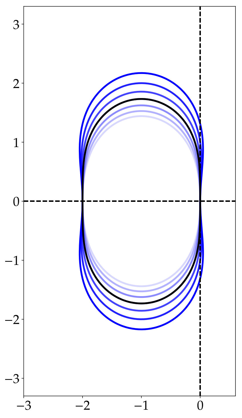 Figure 1
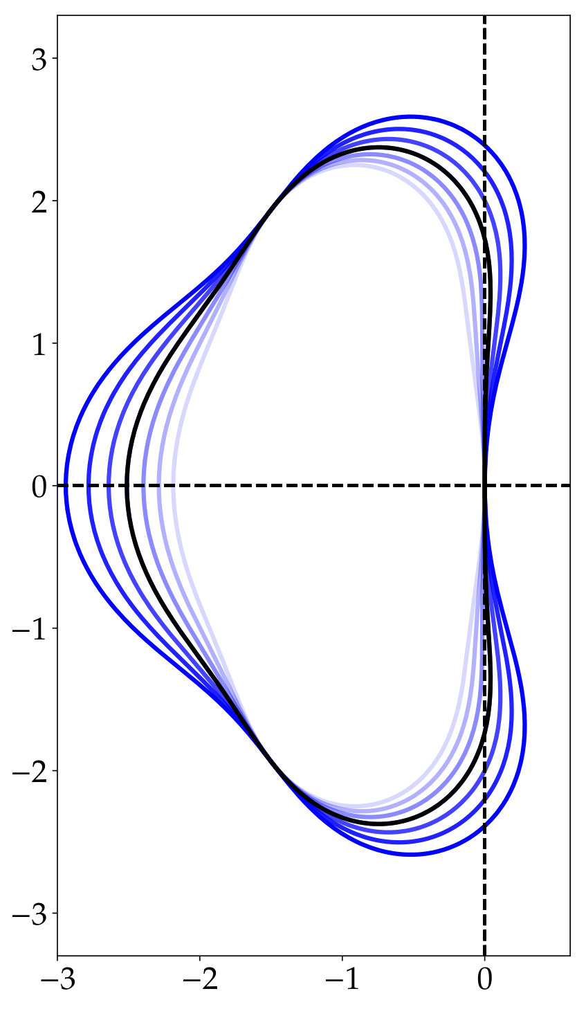 Figure 2
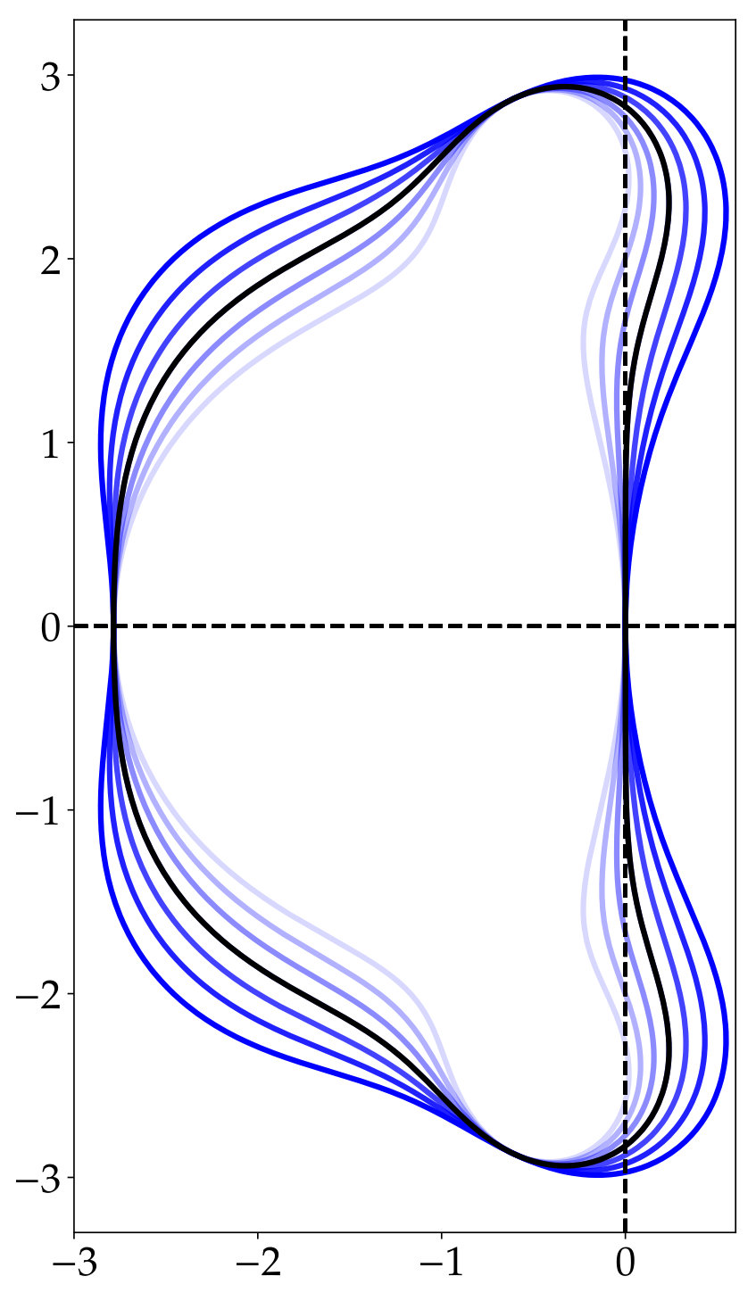 Figure 3
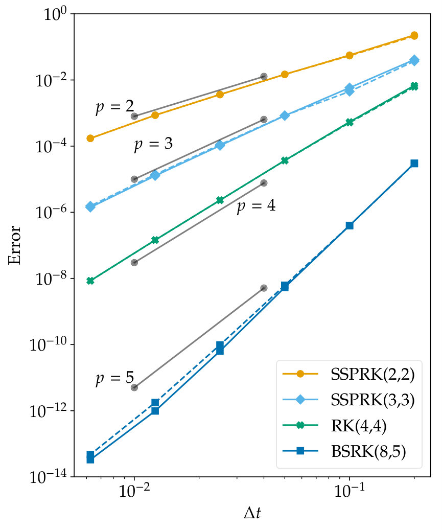 Figure 4
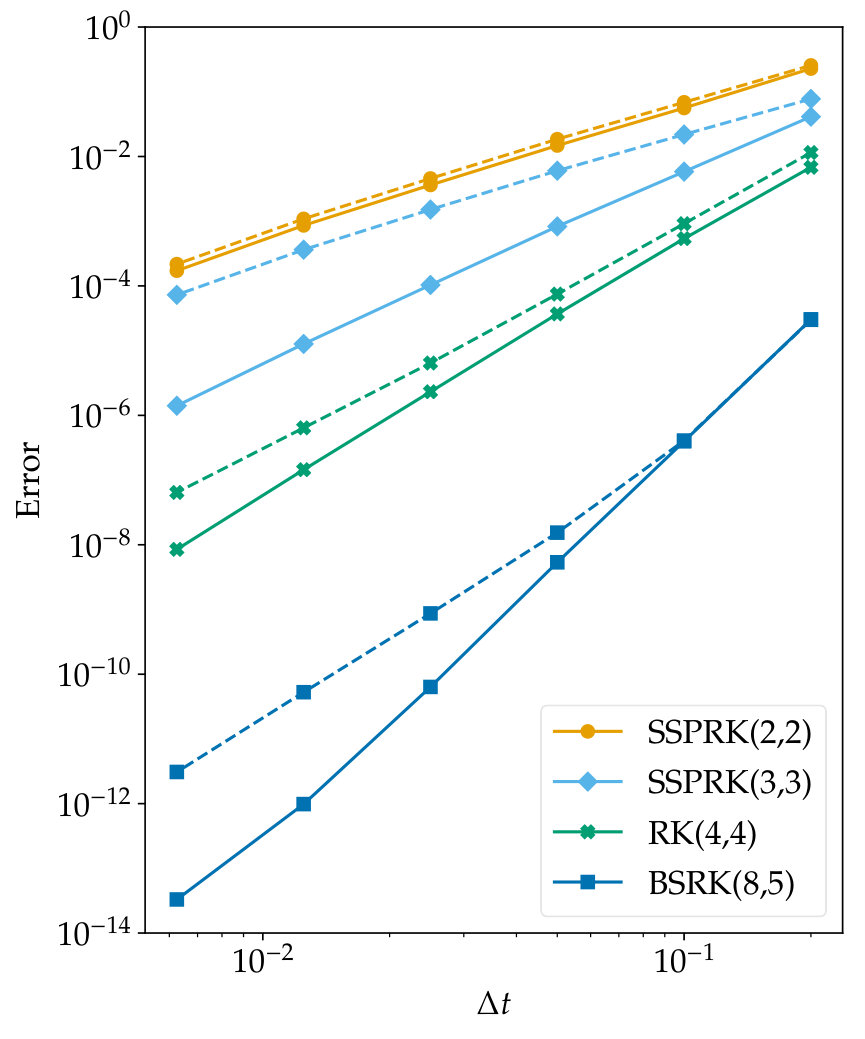 Figure 5
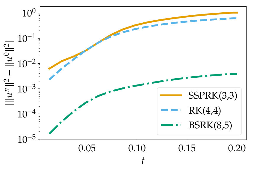 Figure 6
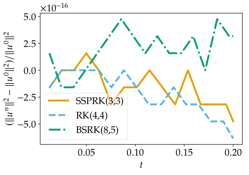 Figure 7
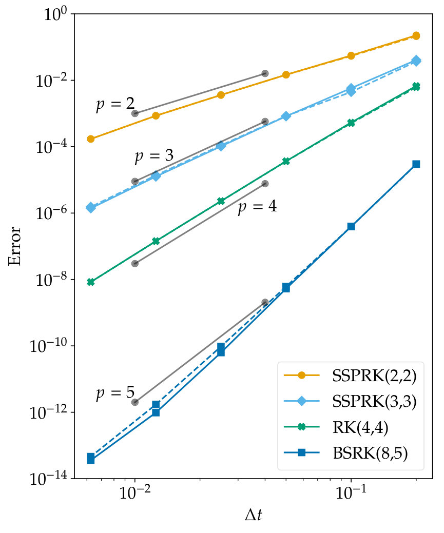 Figure 8
 Figure 9
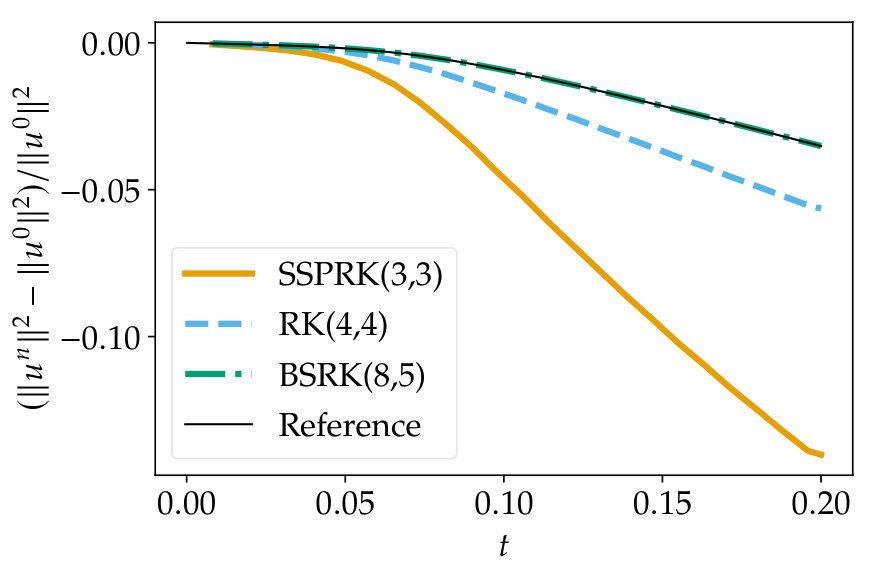 Figure 10
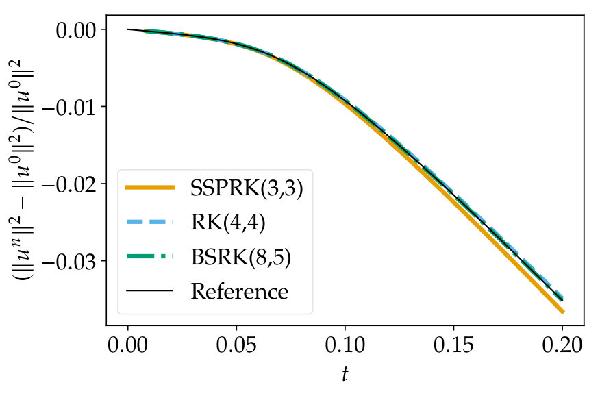 Figure 11
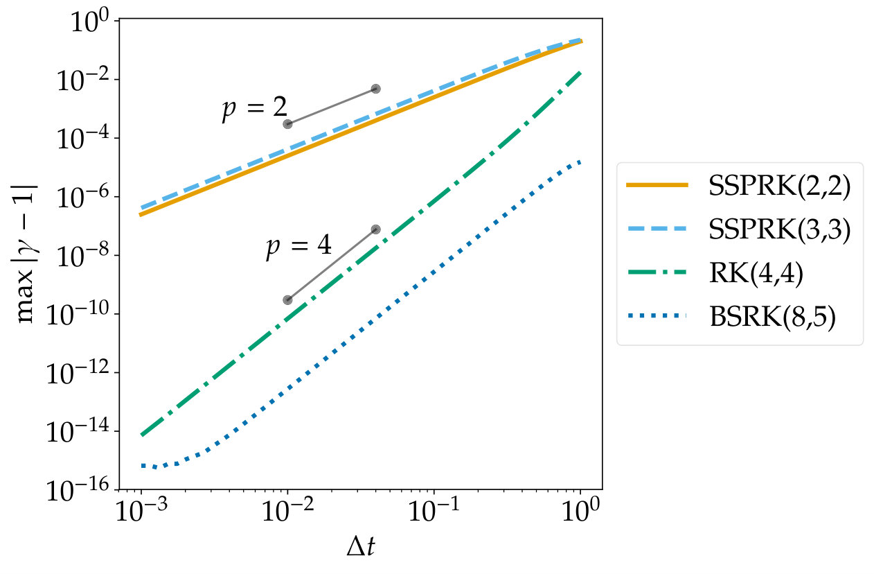 Figure 12
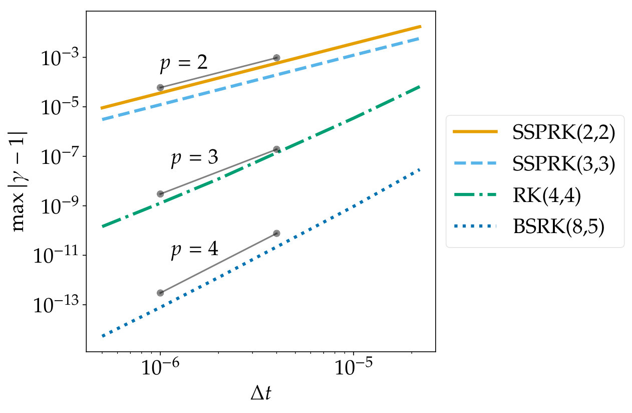 Figure 13
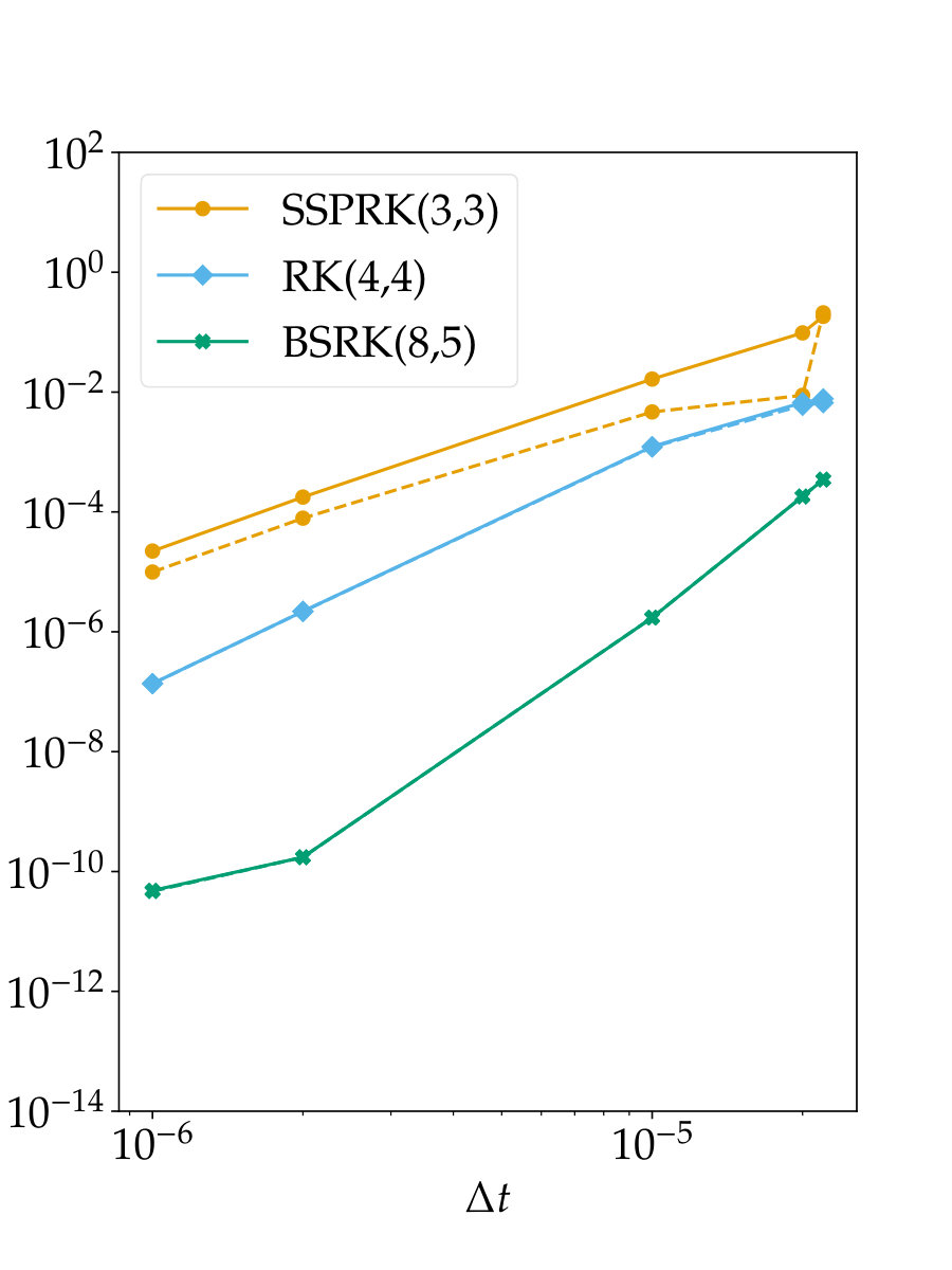 Figure 14
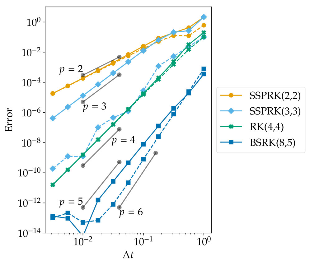 Figure 15
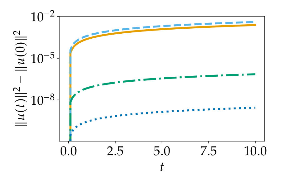 Figure 16
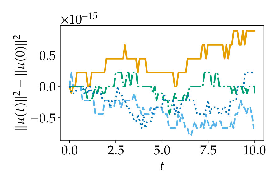 Figure 17
 Figure 18
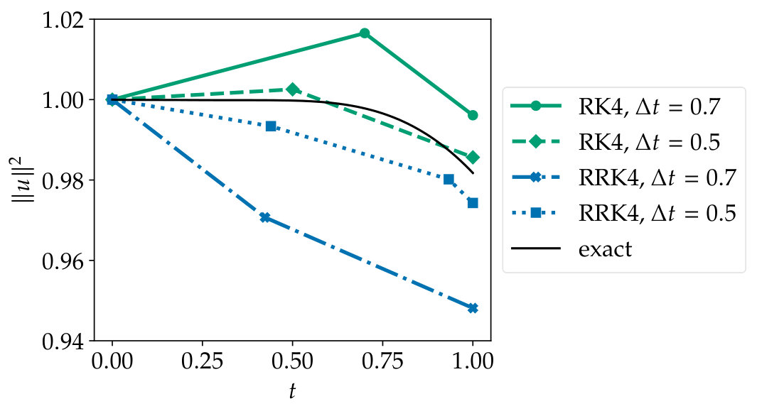 Figure 19
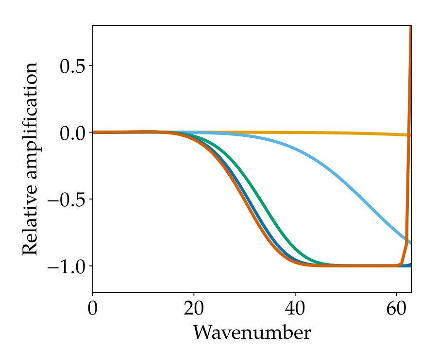 Figure 20
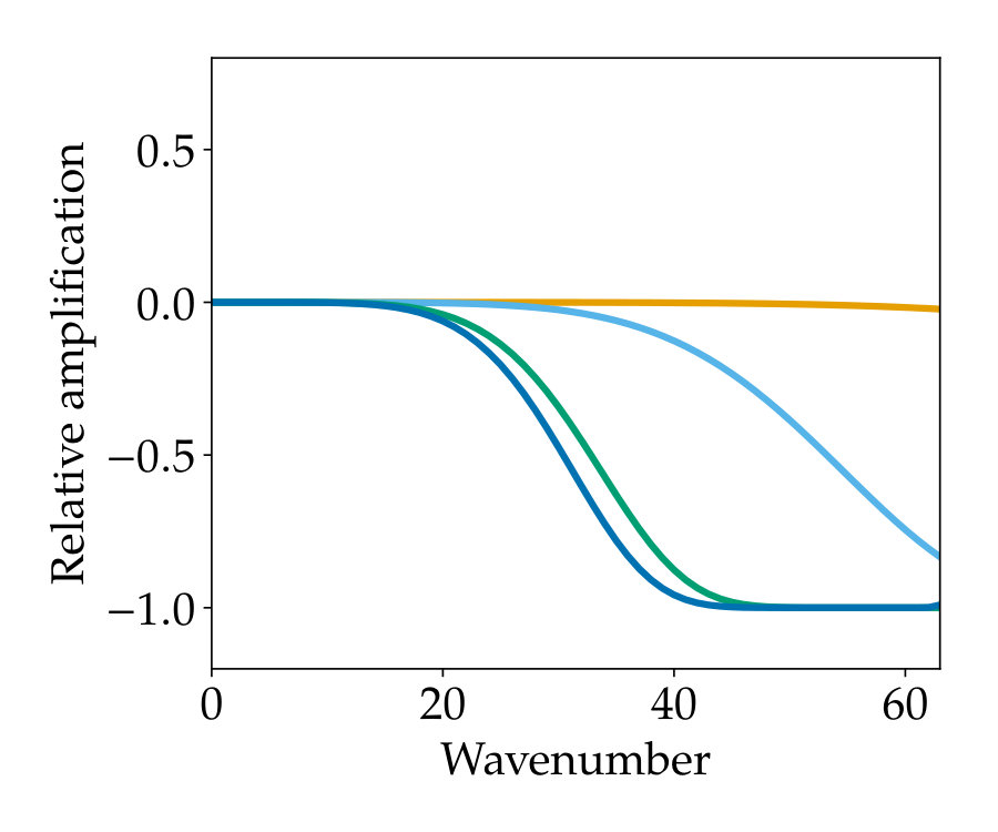 Figure 21
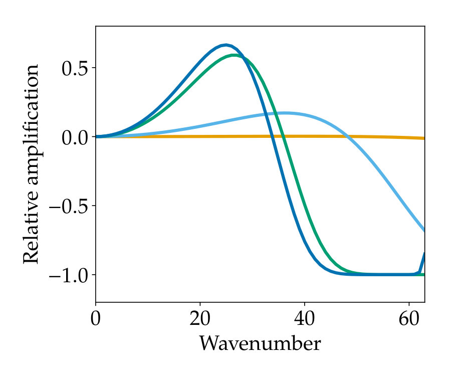 Figure 22
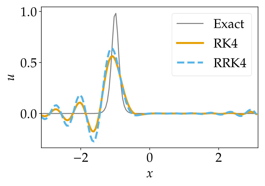 Figure 23
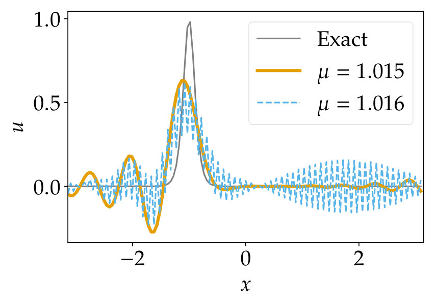 Figure 24
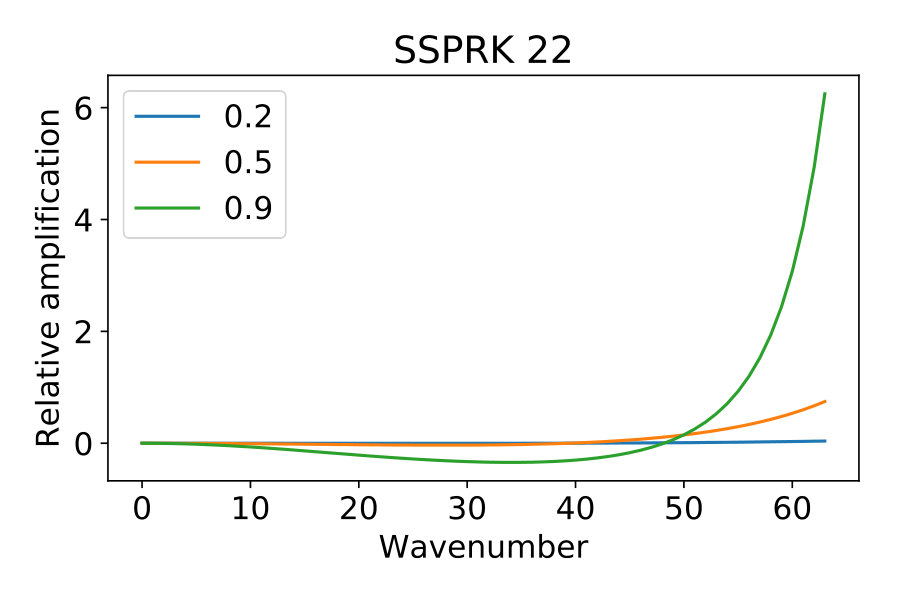 Figure 25
 Figure 26
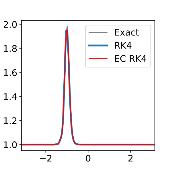 Figure 27
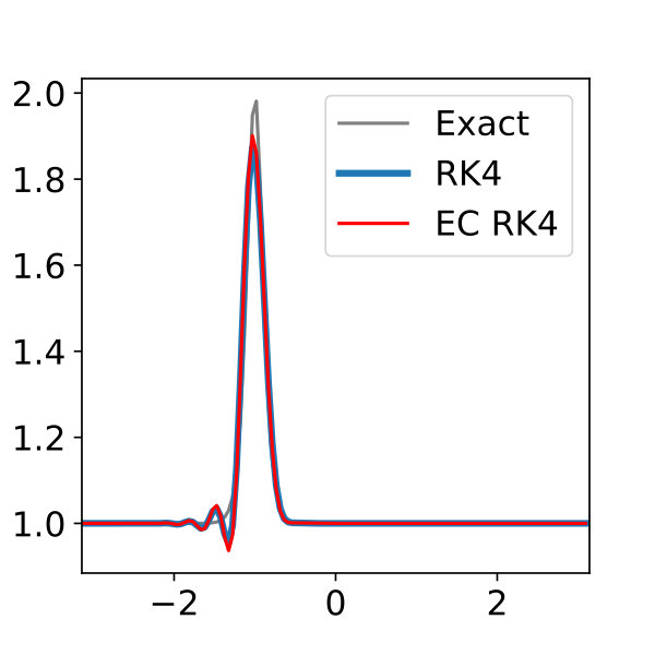 Figure 28
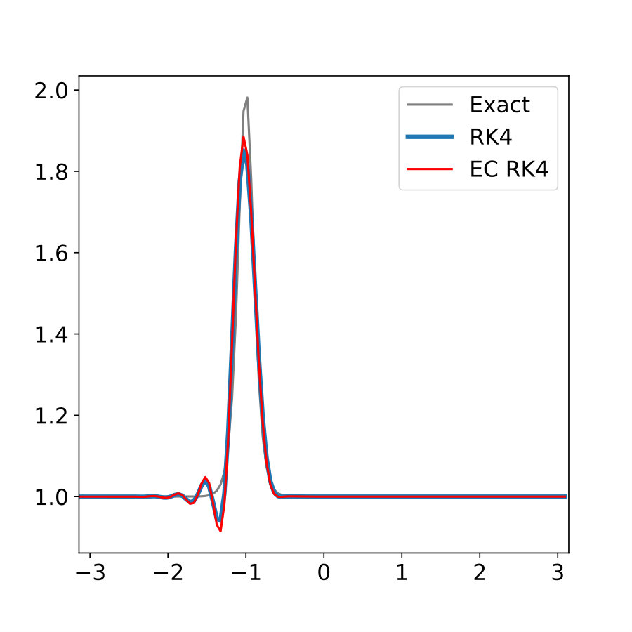 Figure 29
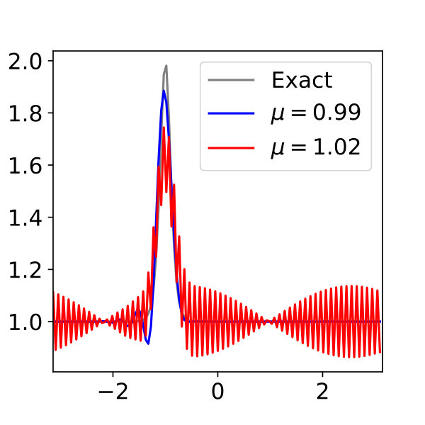 Figure 30
| Method | |
|---|---|
| SSPRK(2,2) | 2 |
| SSPRK(s,2) | s/(s-1) |
| SSPRK(3,3) | 3/2 |
| SSPRK(4,3) | 1 |
| SSPRK(5,3) | 1 |
| SSPRK(9,3) | 1 |
| SSPRK(5,4) | 1.312 |
| SSPRK(10,4) | 25/24 |
Peer Reviews
No public reviews on file for this paper yet. If you reviewed it on a platform where reviews are public (OpenReview, ICLR, NeurIPS, ICML), you can paste yours below so the community can read it here.
Videos
No videos yet. Explain this paper in a talk, walkthrough, or lecture? Add one.
Relaxation Runge-Kutta Methods: Conservation and stability for
Inner-Product Norms
David I. Ketcheson Computer, Electrical, and Mathematical Sciences & Engineering Division, King Abdullah University of Science and Technology, 4700 KAUST, Thuwal 23955, Saudi Arabia. ([email protected])
Abstract
We further develop a simple modification of Runge–Kutta methods that guarantees conservation or stability with respect to any inner-product norm. The modified methods can be explicit and retain the accuracy and stability properties of the unmodified Runge–Kutta method. We study the properties of the modified methods and show their effectiveness through numerical examples, including application to entropy-stability for first-order hyperbolic PDEs.
1 Motivation and background
Consider the initial value problem
[TABLE]
where111We consider real spaces for simplicity, but the methods developed here are also applicable in complex spaces. and . In this work we focus on problems that are dissipative with respect to some inner-product norm:
[TABLE]
Here and throughout, denotes an inner product and the corresponding norm; we will sometimes refer to as energy. For dissipative problems, it is desirable that the numerical solution mimic (2):
[TABLE]
Herein, a method is called monotonicity preserving if it guarantees (3) for all problems satisfying (2).
We say the problem (1) is conservative if
[TABLE]
For such problems it is desirable to discretely conserve energy:
[TABLE]
A method is also called conservative if it guarantees (5) for all problems satisfying (4).
In many applications, numerical conservation or monotonicity preservation are of great importance. Not only do these properties guarantee that the solution remains bounded, but violation of these properties can lead to solutions that are unphysical and qualitatively wrong. Nevertheless, most numerical methods do not enforce these properties exactly, but only up to truncation errors. This is particularly true for explicit Runge–Kutta methods. Even if one considers only linear autonomous systems of ODEs, it has been shown that many explicit Runge–Kutta methods — including the classical 4th-order method — are not even conditionally monotonicity preserving; see [26, 24, 21, 25]. For general nonlinear autonomous systems, no methods of order greater than one are known to be monotonicity preserving [19]. For conservative problems, no explicit Runge–Kutta method of any order can enforce discrete conservation, even for linear autonomous problems. Formulas for the production of a general convex entropy function (which includes the special case of an inner-product norm) have been derived in [18].
Monotonicity preservation for Runge–Kutta methods with respect to an inner-product norm was studied by Higueras [14], with results closely connected to an earlier study of contractivity preservation by Dahlquist & Jeltsch[6]. However, to obtain results for explicit RK methods in that framework, it is necessary to require strict inequality in (2), making the results inapplicable for conservative problems or for typical high-order semi-discretizations of hyperbolic PDEs.
Unconditionally conservative and monotonicity-preserving methods exist, for instance, among the classes of implicit Runge–Kutta and (for Hamiltonian systems) partitioned Runge–Kutta methods; see [12] and references therein.
While classical explicit Runge–Kutta or linear multistep methods cannot preserve general quadratic invariants, some explicit energy-conservative methods have been developed by going outside these traditional classes (as is done also in the present work). Indeed, it is possible to modify any Runge–Kutta method to preserve energy or other first integrals by a technique known as projection; see e.g. [10, 4]. In this approach, at the end of each time step the solution is projected onto a desired set in order to ensure some property like conservation or monotonicity. The approach used in the current work can be viewed as a projection method where the projection is performed along a direction corresponding to the next time step update, but with an additional modification that the size of the time step is also modified. This approach was originally proposed by Dekker & Verwer [7, pp. 265-266], who noted that the classical four-stage RK method could be modified slightly to conserve energy while maintaining its accuracy. The idea was extended in [8] to a restricted class of fourth order methods. This was developed further in [5] by giving a general proof that applying the technique (without the step size adjustment) to a RK method of order results in a method of order at least . Subsequent development in [5, 4, 17] focuses on embedded projection methods; i.e. methods that project in a direction determined by an embedded Runge–Kutta pair. The approach described in the present work could be viewed as a variant in which the “embedded” method is simply the identity map, but with an additional twist that requires reinterpretation of the new step solution as an approximation at a slightly different time.
Like embedded projection methods, the methods proposed here are:
- •
explicit
- •
conditionally conservative and monotonicity-preserving for general nonlinear ODEs
- •
arbitrarily high order accurate
- •
linearly covariant
Furthermore, they do not require partitioning or temporal staggering, and they inherit other useful properties (such as strong stability preservation) of a selected Runge–Kutta method. Preservation of more general (non-inner-product) functionals is also possible with modification similar to that described herein; see [22].
The main contributions of the present work are: first, to further develop these methods that, while not entirely new, seem to have been overlooked; second, to put them on a rigorous footing in terms of accuracy and stability properties; and third, to explore their properties through analysis and numerical experiments.
1.1 Energy evolution by Runge–Kutta methods
A Runge–Kutta method applied to (1) takes the form
[TABLE]
We make the usual assumption that . For convenience we introduce the shorthand
[TABLE]
for the th stage derivative. The change in energy from one step to the next is
[TABLE]
which can be rewritten using (6a) as
[TABLE]
The first sum on the right side of (7) is zero for conservative systems, and it is negative for dissipative systems if for all . However, the remaining two terms may lead to violation of the conservation or monotonicity property. Those two terms can be written together as the bilinear form
[TABLE]
where, letting denote the diagonal matrix with entries ,
[TABLE]
This is the traditional analysis used in studying symplecticity, algebraic stability, and other properties of RK methods (see e.g. [3, 7, 12]). If the matrix is positive semidefinite and the weights are nonnegative, then the method is said to be algebraically stable. Clearly, such methods are unconditionally monotonicity-preserving. If , the method is said to be symplectic; clearly such methods are unconditionally conservative. Certain well-known implicit methods have these properties. However, explicit methods cannot be algebraically stable or symplectic.
2 Relaxation Runge–Kutta methods
The relaxation version of the method (6) is obtained by replacing (6b) with the update formula
[TABLE]
The only difference between (9) and (6b) is the factor that multiplies the step size. We can think of the original Runge–Kutta method (6) as determining only the direction in which the solution will be updated, while the choice of determines how far to step in that direction. From this point of view is similar to the relaxation parameter used in some iterative algebraic solvers, and for this reason we refer to these methods as relaxation Runge–Kutta (RRK) methods.
With this change, (7) becomes
[TABLE]
We can eliminate the last two terms by setting
[TABLE]
so that
[TABLE]
In case the the denominator of (11) vanishes, we have , so we can achieve conservation or monotonicity by taking simply . We thus define in place of (11)
[TABLE]
Because we will interpret as an approximation to the solution at time , it is important that . It is straightforward to show the following:
Lemma 1**.**
Let , let be sufficiently smooth, and let be defined by (12). Then for sufficiently small .
Note that the condition in Lemma 1 holds for all methods of order two or higher.
Remark 1**.**
A more detailed analysis indicates that small enough here means that should be no more than about , where is the Lipschitz constant of . This is also the order of the absolutely stable step size when using any explicit method, so one may expect that using an absolutely stable step size will also yield .
For conservative systems this gives exact energy conservation; for dissipative systems it preserves dissipativity as long as all weights are non-negative.
Theorem 2**.**
Let be the coefficients of a Runge–Kutta method of order at least two. The corresponding relaxation Runge–Kutta method defined by (6a) and (9) with defined by (12) is conservative. If the weights are nonnegative, then the relaxation method is also monotonicity preserving as long as is chosen so that .
Remark 2**.**
The relaxation RK method still conserves linear invariants, which is important for instance in the semi-discretization of hyperbolic conservation laws.
Remark 3**.**
A version of Theorem 2 applicable only to conservative systems appears in [5, Thm. 2.1], along with a formula for that is more computationally efficient (but correct only for conservative systems).
Remark 4**.**
The denominator of the expression for in (11) is simply the norm of the step update, and can be computed with a single inner product. It has been pointed out by Hendrik Ranocha that by solving (7) for the term that is the numerator of the expression for , it can be computed using only inner products [20]. Thus can be computed with just inner products.
The update formula (9) is equivalent to replacing the coefficients in the Runge–Kutta method with . It can also be viewed roughly as taking a Runge–Kutta step of size in place of , but notice that the original step size is still used in the computation of the stages . Both viewpoints (rescaling and rescaling ) will be useful in our analysis.
We will see below in Lemma 4 that, for reasonable values of , is close to unity. Although the proof of this fact is technical, the result itself is not surprising, at least for conservative systems. For such systems, the value of given by (12) is a solution of
[TABLE]
which is a quadratic function of with one root at zero. Given that and that according to (10) for conservative problems, it is natural to expect that has a zero within of unity. The method described here can be viewed as using a line search to determine the step size that solves and thus exactly conserves energy.
For dissipative systems also, we will see that the last two terms in (7) are not important (in the sense of accuracy) to the numerical approximation of the energy evolution; i.e. the term approximates the energy evolution over one step to order :
[TABLE]
2.1 Accuracy
At first glance, the RRK method (given by (6a) with (9)) seems to be not even consistent, since in general. For a classical RK method, the condition , along with higher order conditions, is necessary for local consistency of a given order. But for an RRK method, because the coefficients depend on , we can still obtain high order accuracy if the order conditions are nearly satisfied, which is true if is sufficiently close to unity.
Theorem 3**.**
Let be the coefficients of a Runge–Kutta method of order . Consider the RRK method defined by (6a), (9) and suppose that
[TABLE]
Then:
(IDT method) If the solution is interpreted as an approximation to , the method has order . 2. 2.
(RRK method) If the solution is interpreted as an approximation to , the method has order .
Proof.
First we note that by taking appropriate linear combinations of the usual order conditions, the conditions for a RK method to have order can be written as (see [1])
[TABLE]
where is a set of vectors depending only on whose specific elements are not important here. For the RRK method, we replace with , obtaining the conditions
[TABLE]
Given a method that satisfies (14), clearly (15b) is satisfied as well, while the left hand side of (15a) is . In the error expansion, this value gets multiplied by , so the leading error term is and the method has order .
To prove the second part of Theorem 3, we view the solution given by (9) as an interpolant for the RK solution, evaluated at . The order conditions for this interpolated solution are
[TABLE]
We see that the conditions (16b) and the first bushy-tree condition ((16a) with ) are still exactly fulfilled. The remaining bushy-tree conditions (16a) are not exactly satisfied; for we have, using (14a) and (13),
[TABLE]
In the error expansion, each of these residuals is multiplied by , so that the overall error incurred is . The exponent in this expression is at least for . ∎
It turns out that satisfies the condition required in Theorem 3.
Lemma 4**.**
Let denote the coefficients of a Runge–Kutta method (6) of order , let be a sufficiently smooth function, and let be defined by (12). Then
[TABLE]
We illustrate Lemma 4 in Figure 1, which shows the convergence of to 1 as the step size is reduced for the problem (28). Due to the symmetry of the problem, even faster convergence is observed for some methods.
Remark 5**.**
Lemma 4 was proved in [8, Proposition 4] for the special case of a certain family of four-stage, fourth-order methods.
Before proving Lemma 4 we state the main consistency result, which follows immediately from Theorem 3 and Lemma 4.
Corollary 5**.**
Let be the coefficients of a Runge–Kutta method of order , and consider the RRK method defined by (6a) and (9) with defined by (12).
- •
(IDT method) If the solution is interpreted as an approximation to , the method has order .
- •
(RRK method) If the solution is interpreted as an approximation to , the method has order ; i.e. the solution after one step satisfies
[TABLE]
Remark 6**.**
The first part of Corollary 5 was proved by different means in [5, Thm. 2.1 (ii)].
In order to prove Lemma 4 we use the theory of B-series and follow the notation of [13]. In the remainder of this section, denotes a tree rather than time and denotes the density of a tree rather than the relaxation step length (see [13, Dfn. 2.10]). Let denote the order of tree , and let denote the tree obtained by attaching a new root node to the root of . Let denote the tree obtained by attaching a new root node to the root nodes of as in [13, Dfn. 2.12]. Then
[TABLE]
and
[TABLE]
Finally, let be defined as in [13, Dfn. 2.9]. We recall [13, Thm. 2.13]:
Theorem 6**.**
A Runge–Kutta method is of order iff
[TABLE]
for all trees of order .
Proof of Lemma 4.
We can write where and
[TABLE]
Thus it suffices to show that
[TABLE]
From [13, Thm. II.2.11] we have the Taylor series for the th stage derivative:
[TABLE]
where is the elementary differential corresponding to . Thus can be expressed as a linear combination of inner products of elementary differentials:
[TABLE]
where is the order (number of nodes) of tree , and range over the set of all labelled rooted trees. Here
[TABLE]
Because of the symmetry of the inner product, it is sufficient to show that
[TABLE]
for all pairs of trees satisfying
[TABLE]
We have
[TABLE]
Here we have applied (17) in various places, using the fact that our method is of order and that (due to (19)) the trees in question all have order less than or equal to . ∎
Remark 7**.**
It is possible to prove a generalization of Lemma 4 without the use of B-series; see [22]. The proof above is included here to show a direct approach that is very different from that used in [22].
2.2 Comparison with projection methods
A projection Runge–Kutta method [12, Section IV.4] consists of the traditional Runge–Kutta formula (6) followed by a projection step:
[TABLE]
where is the projection direction and is chosen so that lies on a desired manifold. A relaxation Runge–Kutta method can be viewed as a projection method along the direction with step length . However, the existing formalism for such methods does not include the possibility of interpreting the new solution as an approximation at a time different from . In [5], this projection perspective was applied and it was shown that the resulting method is indeed of order when the original RK method is order . We follow the terminology of [5] and refer to this interpretation as the incremental direction technique, or IDT.
To properly write a relaxation method as a projection method we can write (1) as the equivalent autonomous system of ODEs in the standard way with
[TABLE]
where . The projection of the solution of this problem in the direction requires also projecting the updated value of to obtain the value .
3 Stability properties of explicit relaxation RK methods
All of the results in the previous section apply to general Runge–Kutta methods. In the rest of this work, we focus on explicit methods.
An important question not explicitly answered in the foregoing analysis is how large the step size can be taken in practice. Theorem 2 guarantees unconditional stability for RRK methods applied to any conservative problem, and guarantees stability for dissipative problems as long as the step size is small enough. Due to the overall explicit nature of the methods, we should not expect in either case to obtain accurate results using step sizes much larger than what the original explicit RK method allows; in this respect RRK methods behave similarly to rational Runge–Kutta methods, to which their form is also very similar [27, 11]. In this section we investigate linear stability of RRK methods and also study how the strong stability preserving (SSP) property is affected by the use of RRK methods.
The behavior of an RRK method may be quite challenging to analyze, since depends in a nonlinear way on the method coefficients and the numerical solution itself. On the other hand, over a single step we can think of as a fixed value close to unity, and study the properties of the Runge–Kutta method
[TABLE]
3.1 The stability function
The stability function of a Runge–Kutta method is
[TABLE]
where is vector with all entries equal to unity. Thus the stability function corresponding to one step of the relaxation method (22) is
[TABLE]
Letting denote the coefficients of for an explicit method:
[TABLE]
we have
[TABLE]
Let denote the region of absolute stability of RK method . It turns out that grows as decreases.
Theorem 7**.**
Let be given such that . Then .
Proof.
It is sufficient to show that if for some then . Let ; then clearly implies . ∎
Theorem 7 is illustrated in Figure 2, which shows the stability region for relaxation RK methods with 2–4 stages and order equal to the stage number. Stability region boundaries are shown for different values of in the range . This is an exaggerated range compared to values of that are used in practice; for practical values of , the change in the stability region is visually too small to notice. It is particularly interesting to note that small reductions in lead to significantly enhanced stability along the imaginary axis. Note also that as , the RRK method tends to the identity map and .
Consideration of absolute stability along the imaginary axis leads to the so-called E-polynomial, which for explicit RK methods is
[TABLE]
Clearly the method is stable for such that . Direct calculation shows that for any RRK method of order at least (where ), we have
[TABLE]
The leading terms up to (which vanish for a standard RK method) are positive for , so we see that for every method of order two or higher includes a segment of the imaginary axis containing when . This can be observed for instance in Figure 2(a), where the RK method is unstable over the whole imaginary axis, but for the stability regions include part of the imaginary axis.
3.2 Strong stability preservation
Because the RRK method is only a small perturbation of the original RK method, desirable properties of the original method may remain in effect when using the RRK version. We illustrate this idea by studying strong stability preserving RRK methods.
In the following, denotes the SSP coefficient (or radius of absolute monotonicity) of the Runge–Kutta method with coefficients . Recall that is equal to the largest value such that the method is absolutely monotonic at [9].
For , is a convex combination of and , which implies that for . For many methods, also does not decrease when is taken a little larger than 1.
Lemma 8**.**
Let the RK method with coefficients be absolutely monotonic at . Then the method with is also absolutely monotonic at iff .
Proof.
The conditions for absolute monotonicity of method at can be written (see, e.g. [9, p. 211]
[TABLE]
Conditions (24a) do not depend on , while the first condition of (24b) will hold for any positive multiple of if it holds for . ∎
Theorem 9**.**
Given a RK method with coefficients , we have for , where
[TABLE]
Proof.
Combining Lemma 8 with a standard result on absolute monotonicity (see e.g. [16, Lemma 3.1]) we have that is absolutely monotonic on as long as . Since , we obtain the condition stated in the theorem. ∎
Values of are given in Table 1 for some well-known SSP methods. For all of these methods, direct computation shows that for , while taking leads to a decrease in the SSP coefficient.
4 Numerical examples
For conservative systems, stability is guaranteed under any step size. However, one expects the accuracy to deteriorate significantly if is not close to unity. In the dissipative case, it is possible that becomes negative and stability is lost. A careful examination of the analysis in the previous sections suggests that step sizes on the order of what linearized stability analysis predicts to be stable should be acceptable.
The following Runge–Kutta methods will be used in the numerical experiments.
- •
SSPRK(2,2): Two-stage, second-order SSP method of [23].
- •
SSPRK(3,3): Three-stage, third-order SSP method of [23].
- •
SSPRK(10,4): Ten-stage, fourth-order SSP method of [15].
- •
RK(4,4): Classical four-stage, fourth-order method.
- •
BSRK(8,5): Eight-stage, fifth-order method of [2]. A fixed step size is used and the embedded method is not used.
All of these methods have non-negative weights. We refer to the relaxation version of a method by replacing “RK” with “RRK”; e.g. RRK(4,4).
4.1 Linear, skew-Hermitian system
With this example we investigate the behavior of RRK methods for linear skew-Hermitian problems. For concreteness, we consider the advection equation
[TABLE]
with periodic boundary conditions over a spatial interval of length discretized in space by a Fourier spectral collocation method with points. This results in a linear, constant-coefficient system of ODEs:
[TABLE]
where at evenly spaced points and is the skew-Hermitian Fourier spectral differentiation matrix. Since is normal, the behavior of any RK method on this problem can be characterized simply in terms of the eigenvalues of and the corresponding eigenvectors, which are discrete Fourier modes:
[TABLE]
Let us express the initial data in terms of these modes:
[TABLE]
where is the discrete Fourier transform (DFT) of . Then the exact solution of the semi-discrete system is given by
[TABLE]
Thus the energy associated with each mode is constant in time. Applying a Runge–Kutta method we instead obtain the solution
[TABLE]
where is again the stability function of the method. The energy associated with mode is modified by the factor at each step. The maximum stable step size is the value that guarantees for all . This is just
[TABLE]
where is the length of the method’s imaginary axis stability interval. In the following experiments, we use a step size . Using a given (standard) RK method and , we have absolute stability and the energy of each mode decays. This is illustrated in Figure 3(a), where we solve with and plot the relative change in amplitude
[TABLE]
for each mode, for a range of time step sizes . Due to symmetry we plot only the positive wavenumbers. This figure does not depend on the initial data but only on , where is the total number of time steps taken. For larger values of , the high wavenumber modes are strongly damped.
Now let us consider what happens when applying a relaxation Runge–Kutta method with chosen according to (12) so that energy is conserved. At each step, the energy in mode is modified by the factor . If the initial data is chosen to consist of a single wavenumber , then will take a value such that , and the same value of will be used at every step. For more general initial data, is chosen precisely so that the change in energy when summed over all modes is zero. This value depends on the data, so will be different at each step. Furthermore, at each step some modes will be diminished while others will grow. This is illustrated in Figure 3(b), which is analogous to Figure 3(a) but for the energy-conserving RRK(4,4) method, with initial data taken as white noise; i.e. where the phases are random. We see that high-wavenumber modes are again damped, especially for step sizes close to the stability limit. Meanwhile, some lower-wavenumber modes are amplified in order to preserve the total energy. If we instead take initial data that is reasonably well-resolved, such as
[TABLE]
the resulting amplification curves are nearly indistinguishable from those of the standard RK4 method (Figure 3(a)), as shown in Figure 3(c). This is because most of the energy is in the low-wavenumber modes, which are propagated fairly accurately by the standard RK4 method, so little compensation is need in order to conserve energy. In the latter figure we also plot the amplification for , which is beyond the absolute stability limit. We see that in this case the RRK method greatly amplifies the highest-wavenumber mode.
In Figure 4, we compare the behavior of RK(4,4) and relaxation RK(4,4) (RRK(4,4)) for different values of . For , the methods give similar solutions. Unlike RK(4,4), RRK(4,4) remains stable for . However, taking leads to highly inaccurate and oscillatory approximations.
Remark 8**.**
Even for the linearly unstable value , we have found that remains within less than of unity and the solution never blows up. For much larger values () the value of tends to zero after a few steps and the calculation is never completed.
4.2 A non-normal linear autonomous problem
Here we consider a linear autonomous problem with non-normal right-hand side introduced by Sun & Shu [24]:
[TABLE]
This problem is dissipative, but — as shown in [24] — the classical 4th-order Runge–Kutta method RK(4,4) is not monotone for this problem, no matter how small one takes . To provide a concrete example, we compute , where is the stability polynomial of RK(4,4) and we choose step size . The first singular value of the matrix is approximately . Taking a single step with RK(4,4) and initial condition equal to the first right singular vector thus leads to an increase in the energy, as shown in Figure 5. The increase is even larger for the step size 0.7. In contrast, RRK(4,4) preserves monotonicity with either step size.
4.3 Nonlinear oscillator
Here we consider the problem
[TABLE]
with analytical solution
[TABLE]
Although energy is conserved in the exact solution, the widely used SSPRK(3,3) method of Shu & Osher [23] produces a solution whose energy is monotonically increasing for every positive step size [19]. Similar behavior is observed for several other explicit RK methods we have tested, as shown in Figure 6(a). By applying the modification described in the present work, we obtain instead Figure 6(b), showing that energy is conserved up to roundoff error for all methods.
Figure 7 shows the convergence for each of the standard RK methods (solid lines) and its energy-conserving modification (dashed lines). We see that the relaxation method is in each case on par with or more accurate than the original method.
4.4 Burgers’ equation
We solve the inviscid Burgers’ equation
[TABLE]
on the interval with periodic boundary conditions and initial data
[TABLE]
with the flux-differencing discretization
[TABLE]
where is the numerical flux, defined below. The spatial domain is discretized with 50 equally-spaced points. In the convergence tests below, this spatial discretization is held fixed while the time step is varied, in order to investigate only the temporal convergence.
4.4.1 Energy-conservative semi-discretization
We take the second-order accurate symmetric flux [26]
[TABLE]
which yields a conservative semi-discrete system. Because of the lack of numerical viscosity, the semi-discrete solution is not the vanishing-viscosity solution, but instead develops a dispersive shock.
Energy evolution up to is shown in Figures 8. As expected, standard RK methods all exhibit significant growth or dissipation of energy, while RRK methods preserve energy up to roundoff error. Convergence results at (just before shock formation) are shown in Figure 9, where we compare the IDT approach with the full relaxation approach. All RRK methods achieve the order of accuracy of the corresponding RK method, whereas for IDT methods the convergence rate is reduced by one, as predicted by Theorem 3.
4.4.2 Energy-dissipative semi-discretization
We obtain a dissipative system by adding a centered difference to the flux:
[TABLE]
The amount of dissipation is controlled by . The scheme is still consistent with (29) since the amount of dissipation is proportional to . We take . With this dissipative flux, the solution develops a viscous shock.
Results are shown in Figures 10 and 11. What is most interesting is that applying the relaxation approach dramatically improves the numerical approximation of the global dissipation. Convergence results are similar to those obtained with the conservative flux.
5 Conclusions
The relaxation approach we have proposed seems to be a simple and effective way to make any Runge–Kutta method preserve conservation or dissipativity with respect to an inner-product norm. This can be extended to more general convex functionals; see [22]. While we have focused here on explicit methods, the technique applies to implicit methods as well. Like Runge–Kutta methods, relaxation Runge–Kutta methods automatically preserve linear first integrals. If the original method is equipped with an embedded error estimator or dense output formula, these can be used without modification (other than the rescaling of the step size when determining the dense output times). As we have shown, many SSP RK methods retain the same SSP coefficient when used as RRK methods. The linear stability properties of a method are slightly modified depending on the choice of , but in general the allowable step size for an RRK method is essentially the same as that allowed for the original RK method.
Together these properties make RRK methods an attractive choice for symmetric hyperbolic systems; in combination with entropy-stable spatial discretizations they give a fully-discrete, explicit scheme that is provably entropy stable (for quadratic entropies).
In several experiments we have compared results obtained by viewing as an approximation to (the so-called incremental direction technique, or IDT) versus those obtained by viewing it as an approximation to (the relaxation approach). The main purpose of this comparison is to illustrate our theoretical convergence estimates; it is clear that in practice one should always use the latter interpretation. Comparison with embedded projection methods is planned as future work.
For an RK method with stages, determination of via the formula (12) requires the evaluation of inner products (see Remark 4). For typical high-order discretizations of nonlinear PDEs this cost is negligible compared to the evaluations of required for each step. For simpler applications (such as linear wave equations) the cost may be an important factor. A careful comparison of RRK schemes relative to other time discretizations for linear wave equations is the subject of ongoing work.
6 Acknowledgments
The author is grateful to Hendrik Ranocha for helpful comments on drafts of this work. This work was supported by funding from King Abdullah University of Science & Technology.
The reference list from the paper itself. Each links out to its DOI / PubMed record.
- 1[1] Peter Albrecht. The Runge-Kutta Theory in a Nutshell. SIAM Journal on Numerical Analysis , 33(5):1712 – 1735, 1996.
- 2[2] P Bogacki and Lawrence F Shampine. An efficient Runge-Kutta (4, 5) pair. Computers & Mathematics with Applications , 32(6):15–28, 1996.
- 3[3] Kevin Burrage and John C Butcher. Stability criteria for implicit Runge–Kutta methods. SIAM Journal on Numerical Analysis , 16(1):46–57, 1979.
- 4[4] M Calvo, MP Laburta, JI Montijano, and L Rández. Projection methods preserving Lyapunov functions. BIT Numerical Mathematics , 50(2):223–241, 2010.
- 5[5] Manuel Calvo, D Hernández-Abreu, Juan I Montijano, and Luis Rández. On the preservation of invariants by explicit Runge-Kutta methods. SIAM Journal on Scientific Computing , 28(3):868–885, 2006.
- 6[6] Germund Dahlquist and Rolf Jeltsch. Reducibility and contractivity of Runge-Kutta methods revisited. Bit Numerical Mathematics , 46:567–587, 2006.
- 7[7] K. Dekker and J. G. Verwer. Stability of Runge-Kutta methods for stiff nonlinear differential equations , volume 2 of CWI Monographs . North-Holland Publishing Co., 1984.
- 8[8] N Del Buono and C Mastroserio. Explicit methods based on a class of four stage fourth order Runge-Kutta methods for preserving quadratic laws. Journal of Computational and Applied Mathematics , 140(1-2):231–243, 2002.