Resolved Molecular Gas and Star Formation Properties of the Strongly Lensed z=2.26 Galaxy SDSS J0901+1814
Chelsea E. Sharon, Amitpal S. Tagore, Andrew J. Baker, Jesus Rivera,, Charles R. Keeton, Dieter Lutz, Reinhard Genzel, David J. Wilner, Erin K. S., Hicks, Sahar S. Allam, and Douglas L. Tucker

TL;DR
This study uses high-resolution observations of a strongly-lensed galaxy at z=2.26 to analyze its molecular gas, star formation properties, and spatially resolved star formation efficiency, revealing it as a massive, nearly face-on disk with elevated star formation efficiency.
Contribution
It provides the first detailed spatially resolved analysis of molecular gas and star formation in a strongly-lensed galaxy at z=2.26, including lensing potential constraints and source-plane reconstructions.
Findings
SDSS J0901+1814 is a massive, nearly face-on disk galaxy.
The galaxy has a star formation rate of about 268 M_sun/yr.
The Schmidt-Kennicutt relation index is approximately 1.54, possibly affected by lensing.
Abstract
We present ~1" resolution (~2 kpc in the source plane) observations of the CO(1-0), CO(3-2), Halpha, and [N II] lines in the strongly-lensed z=2.26 star-forming galaxy SDSS J0901+1814. We use these observations to constrain the lensing potential of a foreground group of galaxies, and our source-plane reconstructions indicate that SDSS J0901+1814 is a nearly face-on (i~30 degrees) massive disk with r_{1/2}>~4 kpc for its molecular gas. Using our new magnification factors (mu_tot~30), we find that SDSS J0901+1814 has a star formation rate (SFR) of 268^{+63}_{-61} M_sun/yr, M_gas=(1.6^{+0.3}_{-0.2})x10^11x(alpha_CO/4.6) M_sun, and M_star=(9.5^{+3.8}_{-2.8})x10^10 M_sun, which places it on the star-forming galaxy "main sequence." We use our matched high-angular resolution gas and SFR tracers (CO and Halpha, respectively) to perform a spatially resolved (pixel-by-pixel) analysis of SDSS…
Click any figure to enlarge with its caption.
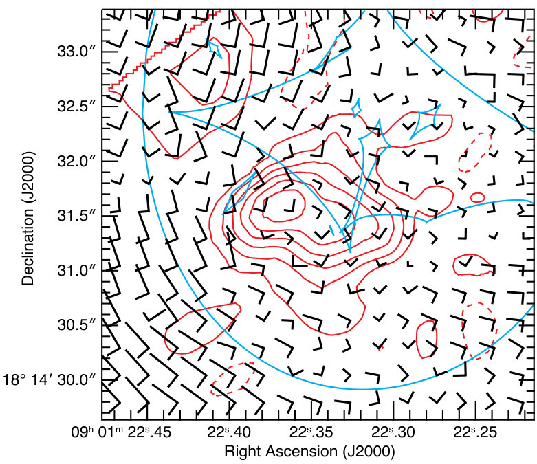 Figure 1
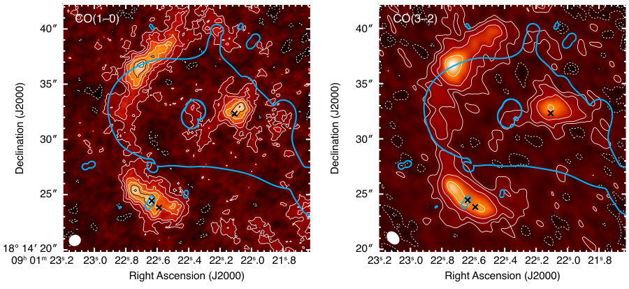 Figure 2
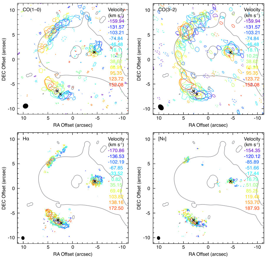 Figure 3
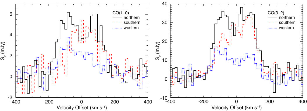 Figure 4
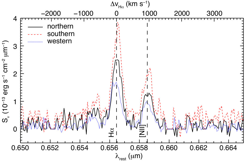 Figure 5
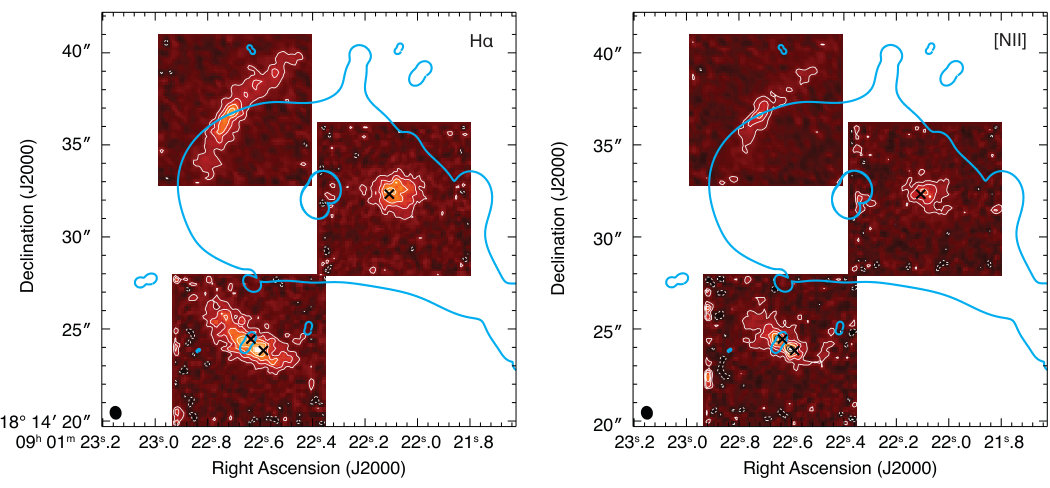 Figure 6
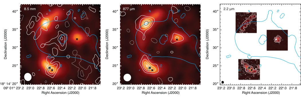 Figure 7
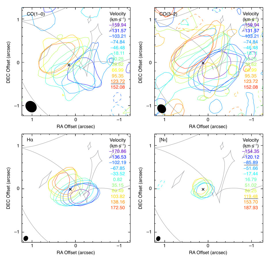 Figure 8
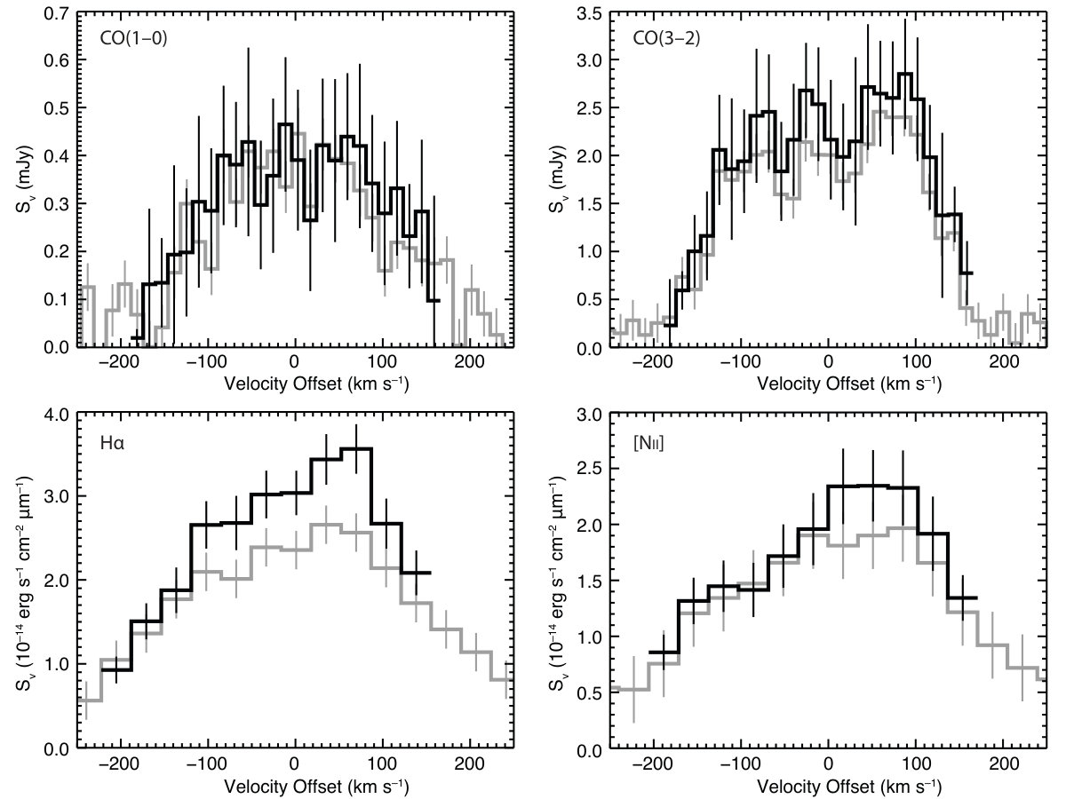 Figure 9
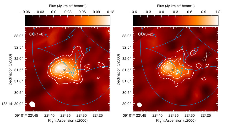 Figure 10
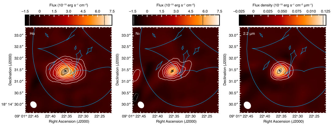 Figure 11
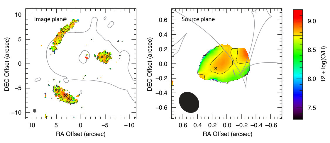 Figure 12
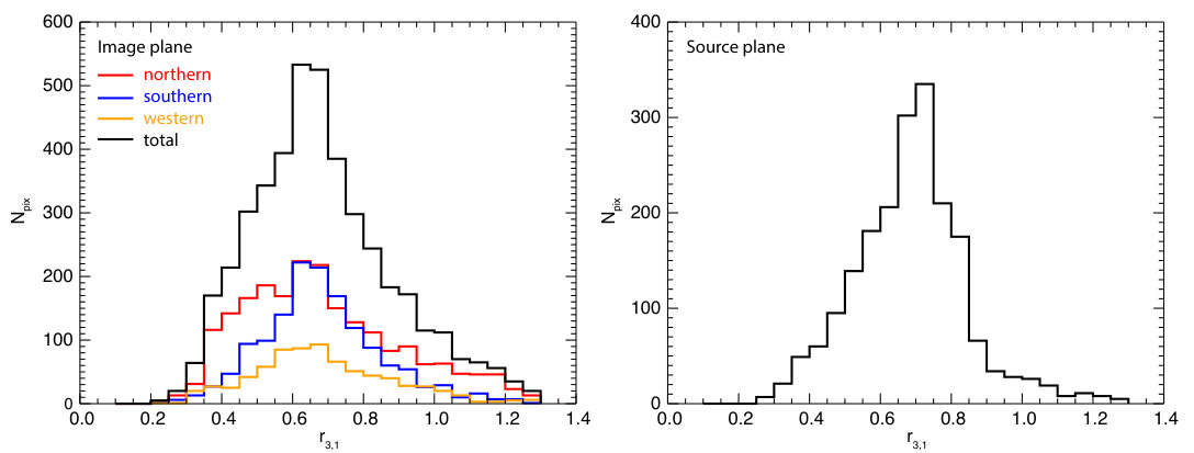 Figure 13
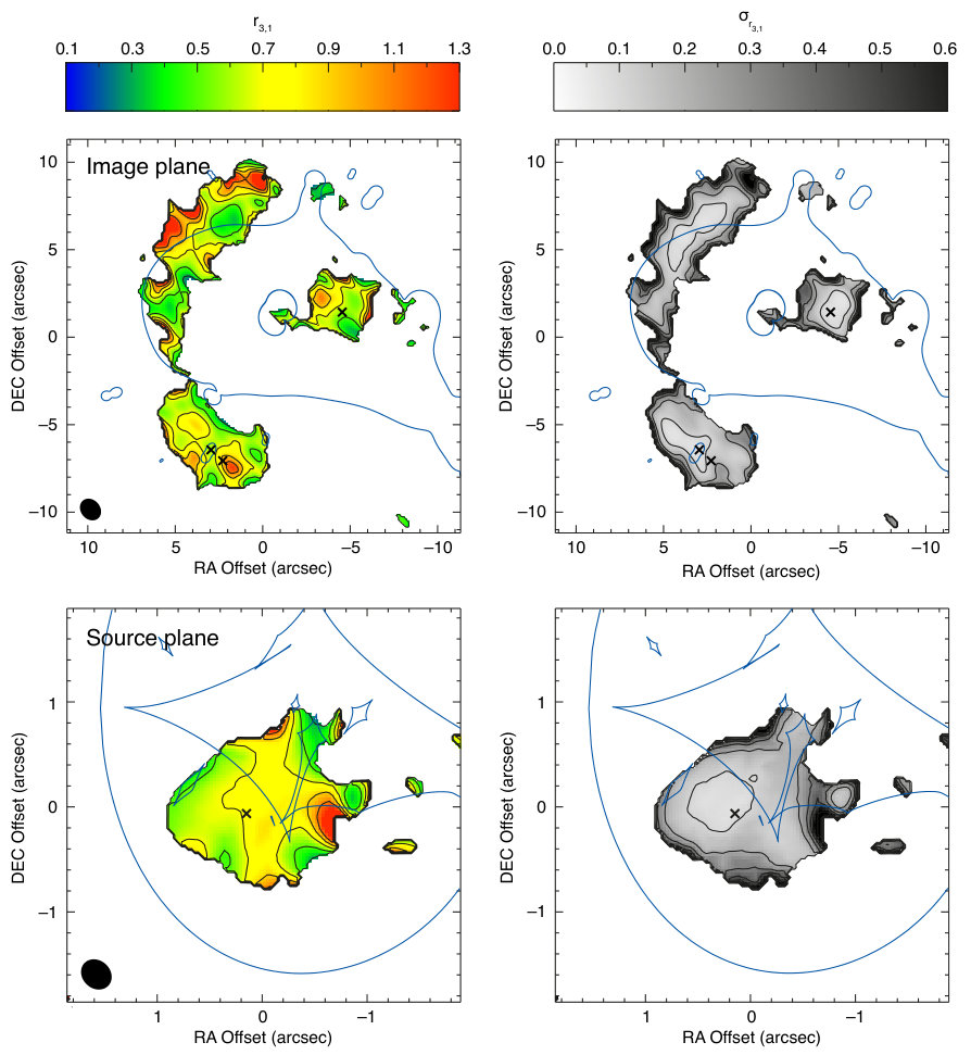 Figure 14
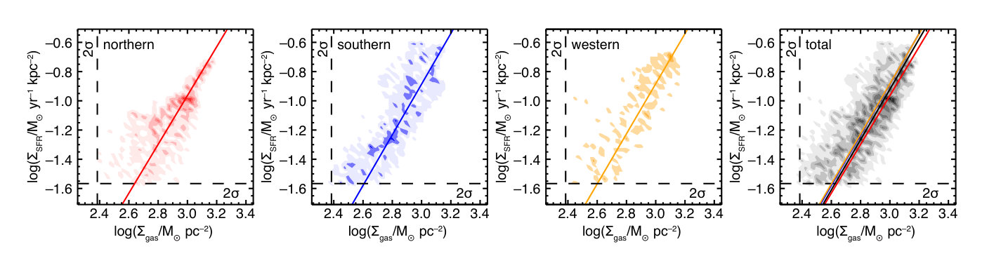 Figure 15
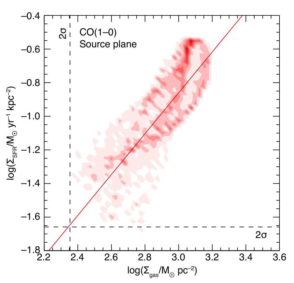 Figure 16
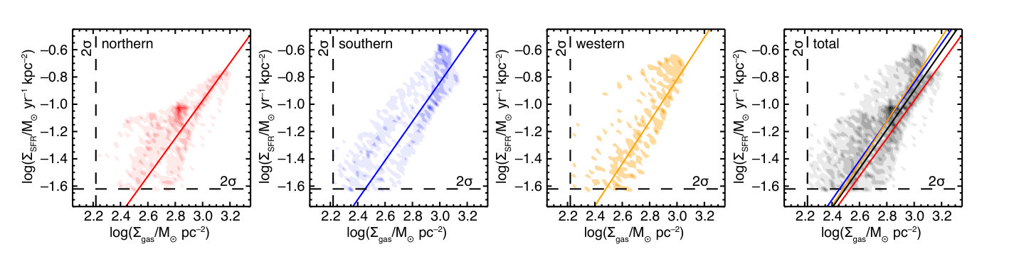 Figure 17
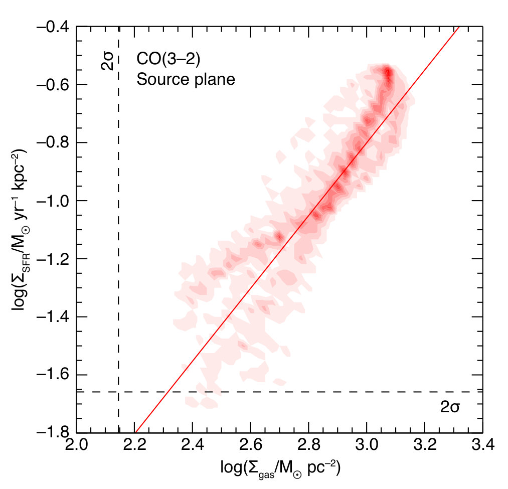 Figure 18
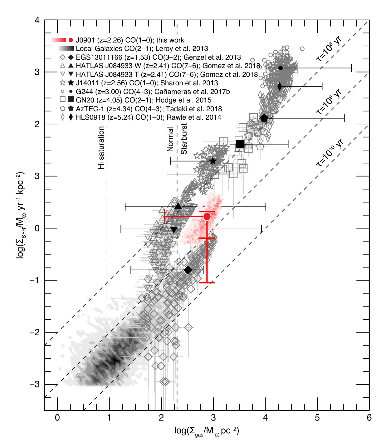 Figure 19
 Figure 20
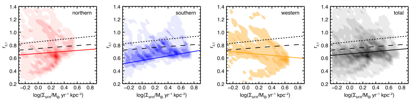 Figure 21
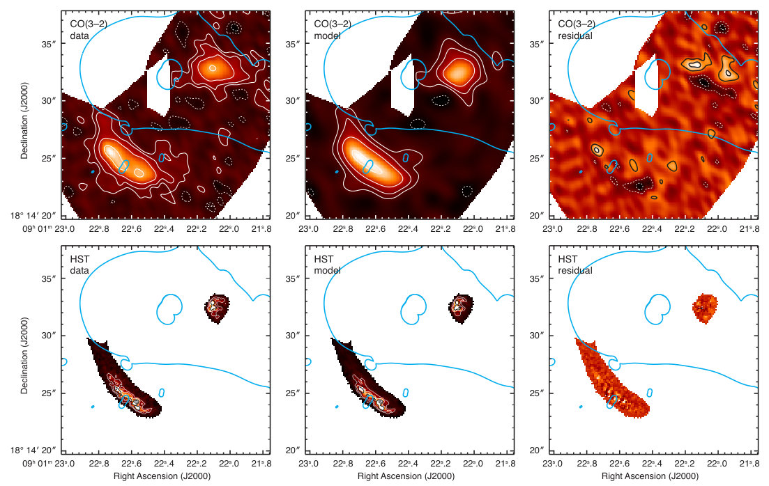 Figure 22
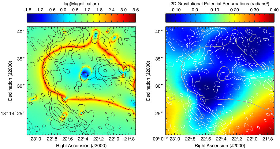 Figure 23
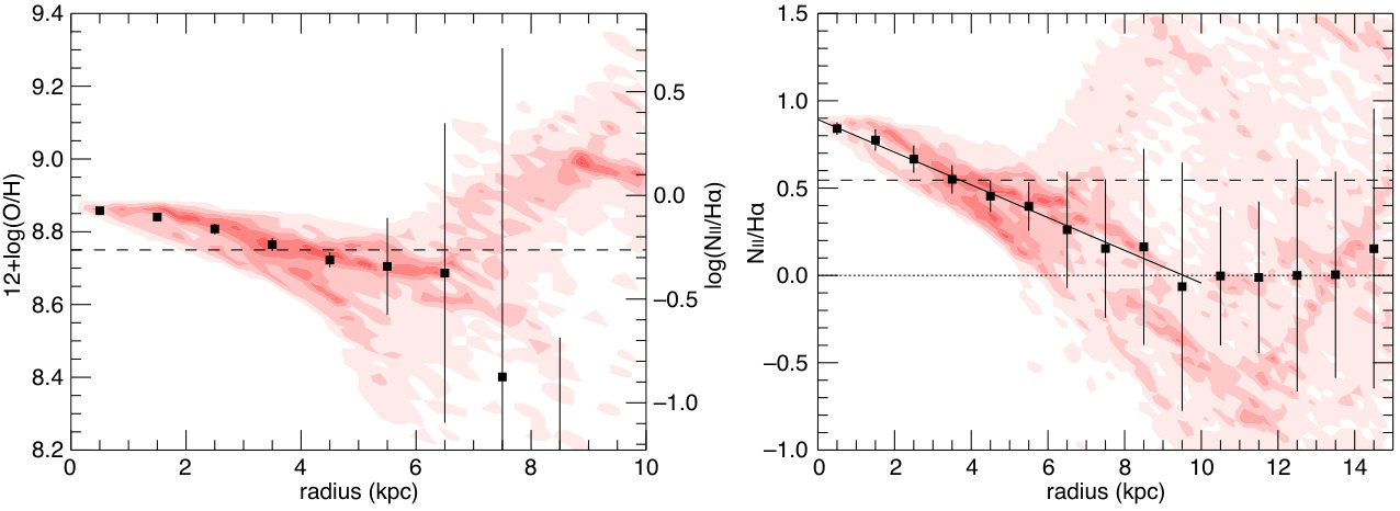 Figure 24
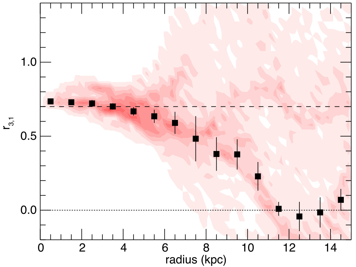 Figure 25
| Configuration | Date | Weather | |
|---|---|---|---|
| Max. Baseline | |||
| D | 2010 April 3 | 17 | Clear |
| 1.031 km | 2010 April 15 | 20 | Clear |
| 2010 May 4 | 19 | Clear | |
| 2010 May 8 | 19 | Average sky cover 25%; mixed clouds | |
| 2010 May 15 | 20 | Sky cover 20%; cumuliform clouds | |
| B | 2011 February 14 | 26 | Sky cover ; stratiform clouds |
| 10.306 km | |||
| C | 2012 January 29 | 26 | Clear |
| 3.289 km | 2012 January 30 | 25 | Clear |
| 2012 January 31 | 25 | Clear | |
| 2012 March 26 | 25 | Sky cover 90%; stratiform clouds | |
| 2012 March 30 | 27 | Sky cover 20%; stratiform clouds |
| Line/Map | Parameter | Units | North | South | West | Total |
|---|---|---|---|---|---|---|
| CO(1–0) | ||||||
| natural | bbThe total line luminosities are magnification corrected assuming the corresponding magnification factors listed in Table 5 (i.e. the “natural” magnification factors calculated using the native resolution data presented in the bulk of this table, or the “matched” magnification factors for the CO(1–0) data -clipped to create the matching resolution datasets). | |||||
| CO(1–0) | ||||||
| matched | bbThe total line luminosities are magnification corrected assuming the corresponding magnification factors listed in Table 5 (i.e. the “natural” magnification factors calculated using the native resolution data presented in the bulk of this table, or the “matched” magnification factors for the CO(1–0) data -clipped to create the matching resolution datasets). | |||||
| CO(3–2) | ||||||
| bbThe total line luminosities are magnification corrected assuming the corresponding magnification factors listed in Table 5 (i.e. the “natural” magnification factors calculated using the native resolution data presented in the bulk of this table, or the “matched” magnification factors for the CO(1–0) data -clipped to create the matching resolution datasets). | ||||||
| H | ||||||
| bbThe total line luminosities are magnification corrected assuming the corresponding magnification factors listed in Table 5 (i.e. the “natural” magnification factors calculated using the native resolution data presented in the bulk of this table, or the “matched” magnification factors for the CO(1–0) data -clipped to create the matching resolution datasets). | ||||||
| [N ii] | ||||||
| bbThe total line luminosities are magnification corrected assuming the corresponding magnification factors listed in Table 5 (i.e. the “natural” magnification factors calculated using the native resolution data presented in the bulk of this table, or the “matched” magnification factors for the CO(1–0) data -clipped to create the matching resolution datasets). | ||||||
| aa upper limit assuming a point-like flux distribution. | ||||||
| Line/Map | Parameter | North | South | West | Total |
|---|---|---|---|---|---|
| CO(1–0) | aaIn units of . | / | / | ||
| natural | FWHM bbIn units of . | / | / | ||
| bbIn units of . | / | / | |||
| CO(1–0) | aaIn units of . | / | / | ||
| matched | FWHMbbIn units of . | / | / | ||
| bbIn units of . | / | / | |||
| CO(3–2) | aaIn units of . | / | / | / | |
| FWHM bbIn units of . | / | / | / | ||
| bbIn units of . | / | / | / | ||
| ccIn units of . | |||||
| FWHMbbIn units of . | |||||
| bbIn units of . | |||||
| [Nii] | ccIn units of . | ||||
| FWHM bbIn units of . | |||||
| bbIn units of . |
| Object(s) | Model | RA | DEC | ||||||
|---|---|---|---|---|---|---|---|---|---|
| (′′) | (′′) | () | (′′) | (′′) | |||||
| Group halo | SPLE | ||||||||
| Central galaxies | SIS | ||||||||
| SIS | |||||||||
| Southern perturber | p-Jaffe | ||||||||
| Other galaxies | SIS | ||||||||
| SIS | |||||||||
| SIS | |||||||||
| SIS | |||||||||
| SIS | |||||||||
| SIS | |||||||||
| SIS | |||||||||
| SIS | |||||||||
| SIS | |||||||||
| SIS | |||||||||
| SIS | |||||||||
| SIS | |||||||||
| SIS | |||||||||
| SIS |
| Transition | Map | North | South | West | Total |
|---|---|---|---|---|---|
| CO(1–0) | natural | ||||
| matched | |||||
| CO(3–2) | natural | ||||
| matched | |||||
| natural | |||||
| matched | |||||
| [N ii] | natural | ||||
| matched | |||||
| natural | |||||
| matched |
| Model | Parameter | Transition | ||
|---|---|---|---|---|
| CO(1–0) | CO(3–2) | |||
| Exponential disk | R.A. | |||
| Dec. | ||||
| P.A. | ||||
| 1.2 | 0.97 | |||
| Gaussian | R.A. | |||
| Dec. | ||||
| P.A. | ||||
| Image | line | |||||
|---|---|---|---|---|---|---|
| North | CO(1–0) | |||||
| CO(1–0)m | ||||||
| CO(3–2) | ||||||
| CO(3–2)m | ||||||
| South | CO(1–0) | |||||
| CO(1–0)m | ||||||
| CO(3–2) | ||||||
| CO(3–2)m | ||||||
| West | CO(1–0) | |||||
| CO(1–0)m | ||||||
| CO(3–2) | ||||||
| CO(3–2)m | ||||||
| Total | CO(1–0) | |||||
| CO(1–0)m | ||||||
| CO(3–2) | ||||||
| CO(3–2)m | ||||||
| De-lensed | CO(1–0)m | |||||
| CO(3–2)m |
| Image | |||
|---|---|---|---|
| North | |||
| South | |||
| West | |||
| Total | |||
| De-lensed |
Peer Reviews
No public reviews on file for this paper yet. If you reviewed it on a platform where reviews are public (OpenReview, ICLR, NeurIPS, ICML), you can paste yours below so the community can read it here.
Videos
No videos yet. Explain this paper in a talk, walkthrough, or lecture? Add one.
Resolved Molecular Gas and Star Formation Properties of the Strongly Lensed Galaxy SDSS J0901+1814111Based on observations carried out with the IRAM Plateau de Bure Interferometer. IRAM is supported by INSU/CNRS (France), MPG (Germany) and IGN (Spain).
Chelsea E. Sharon
Yale-NUS College, Singapore, 138527
Department of Physics & Astronomy, McMaster University, Hamilton, ON, L8S-4M1, Canada
Amitpal S. Tagore
Jodrell Bank Centre for Astrophysics, The University of Manchester, Manchester, M13 9PL, UK
Andrew J. Baker
Department of Physics and Astronomy, Rutgers, the State University of New Jersey, Piscataway, NJ, 08854-8019, USA
Jesus Rivera
Department of Physics and Astronomy, Rutgers, the State University of New Jersey, Piscataway, NJ, 08854-8019, USA
Charles R. Keeton
Department of Physics and Astronomy, Rutgers, the State University of New Jersey, Piscataway, NJ, 08854-8019, USA
Dieter Lutz
Max-Planck-Institut für extraterrestrische Physik (MPE), Giessenbachstr. 1, 85748 Garching, Germany
Reinhard Genzel
Max-Planck-Institut für extraterrestrische Physik (MPE), Giessenbachstr. 1, 85748 Garching, Germany
David J. Wilner
Harvard-Smithsonian Center for Astrophysics, Cambridge, MA, 02138, USA
Erin K. S. Hicks
Department of Physics and Astronomy, University of Alaska, Anchorage, AK, 99508, USA
Sahar S. Allam
Center for Particle Astrophysics, Fermi National Accelerator Laboratory, P.O. Box 500, Batavia, IL, 60510, USA
Douglas L. Tucker
Center for Particle Astrophysics, Fermi National Accelerator Laboratory, P.O. Box 500, Batavia, IL, 60510, USA
(Accepted to ApJ 5/17/2019)
Abstract
We present resolution ( in the source plane) observations of the CO(1–0), CO(3–2), , and [N ii] lines in the strongly-lensed star-forming galaxy SDSS J0901+1814. We use these observations to constrain the lensing potential of a foreground group of galaxies, and our source-plane reconstructions indicate that SDSS J0901+1814 is a nearly face-on () massive disk with for its molecular gas. Using our new magnification factors (), we find that SDSS J0901+1814 has a star formation rate (SFR) of , , and , which places it on the star-forming galaxy “main sequence.” We use our matched high-angular resolution gas and SFR tracers (CO and , respectively) to perform a spatially resolved (pixel-by-pixel) analysis of SDSS J0901+1814 in terms of the Schmidt-Kennicutt relation. After correcting for the large fraction of obscured star formation (), we find SDSS J0901+1814 is offset from “normal” star-forming galaxies to higher star formation efficiencies independent of assumptions for the CO-to- conversion factor. Our mean best-fit index for the Schmidt-Kennicutt relation for SDSS J0901+1814, evaluated with different CO lines and smoothing levels, is ; however, the index may be affected by gravitational lensing, and we find when analyzing the source-plane reconstructions. While the Schmidt-Kennicutt index largely appears unaffected by which of the two CO transitions we use to trace the molecular gas, the source-plane reconstructions and dynamical modeling suggest that the CO(1–0) emission is more spatially extended than the CO(3–2) emission.
galaxies: high-redshift—galaxies: individual (SDSS J0901+1814)—galaxies: ISM—galaxies: starburst—galaxies: star formation—ISM: molecules
1 Introduction
Star forming galaxies at high redshift have been selected using a variety of methods, most notably on the basis of rest-ultraviolet (UV) colors (e.g., Lyman break galaxies, LBGs; Steidel et al. 1996; Giavalisco 2002) and large (observed frame) submillimeter fluxes (e.g., submillimeter galaxies, SMGs; Blain et al. 2002; Casey et al. 2014). Historically, galaxies selected using these two methods have been described as two separate populations, with UV-bright galaxies characterized as “normal” galaxies at high redshifts (mostly disks, and falling along a star-forming “main sequence” (MS) in star formation rate (SFR) vs. stellar mass; e.g, Förster Schreiber et al. 2006; Genzel et al. 2006; Bouché et al. 2007; Wright et al. 2007; Noeske et al. 2007; Elbaz et al. 2007; Daddi et al. 2007; Genzel et al. 2008; Förster Schreiber et al. 2009; Wisnioski et al. 2015) whose SFRs are an order of magnitude lower than those of dusty starbursts that are SMGs (e.g., Rodighiero et al., 2011). However, fits to spectral energy distributions (SEDs; e.g., Wuyts et al. 2011), the decomposition of many of the brightest SMGs into multiples, and stacking (e.g., Lindner et al., 2012; Decarli et al., 2014; Walter et al., 2014) suggest there is substantial overlap in the underlying physical properties of UV- and IR-bright high- galaxies, at least for higher masses.
Despite the increasing evidence of overlap between these populations, comparing their directly observable properties remains difficult. The substantial dust masses that give SMGs their large far-infrared (FIR) luminosities obscure their UV-emission (e.g., Smail et al., 2002; Hodge et al., 2012), including common short-wavelength SFR tracers such as . Similarly, UV-bright galaxies are comparatively dust and gas poor, and therefore frequently require substantial investments of telescope time and/or magnification from gravitational lensing to achieve mere detections of dust and molecular gas (e.g., Baker et al. 2001, 2004; Coppin et al. 2007; Daddi et al. 2010b; Saintonge et al. 2013; Dessauges-Zavadsky et al. 2015). Only recently have larger samples of high-redshift optical/UV color-selected galaxies been detected in CO (e.g., Tacconi et al. 2013; Freundlich 2017; see also: Genzel et al. 2015; Tacconi et al. 2017 and references therein), the canonical tracer of molecular gas, in numbers comparable to those of dusty galaxies (see Carilli & Walter 2013 for a review of gas in high-redshift galaxies). Of the UV or optical color-selected galaxies with CO detections, few have spatially resolved or multi- CO detections (e.g., Genzel et al., 2013). With the wide bandwidths and the sensitivities of telescopes like the Atacama Large Millimeter/submillimeter Array, it has been suggested that dust continuum measurements may be a more efficient way to measure the masses of galaxies’ interstellar media (ISMs; e.g., Scoville et al. 2014, 2016), including their molecular gas components, even for UV-bright/dust-poor systems. However, using different observables to trace the same intrinsic galaxy parameter (e.g., infrared vs. UV-tracers of the total SFR, or dust vs. CO tracers of the molecular gas) may generate false differences between galaxy populations due to systematic factors like extinction or AGN contamination (Kennicutt & Evans 2012).
The lack of data at complementary wavelengths also makes resolved multi-wavelength analyses applied to low-redshift galaxies, such as the Schmidt-Kennicutt relation (the correlation between galaxies’ SFR and gas mass surface densities; e.g., Schmidt 1959; Kennicutt 1989, 1998) significantly less common at high redshift. High-resolution CO observations are critical for evaluating where high-redshift galaxies fall on the true surface density version of the Schmidt-Kennicutt relation, where and can be compared on a pixel-by-pixel basis within individual galaxies (as done for local galaxies; e.g., Kennicutt et al. 2007; Bigiel et al. 2008; Wei et al. 2010; Bigiel et al. 2011; Leroy et al. 2013). Many high-redshift analyses use star formation and gas properties averaged over the entire galaxy (e.g., Kennicutt, 1989; Buat et al., 1989; Kennicutt, 1998; Genzel et al., 2010; Daddi et al., 2010a; Tacconi et al., 2013) or avoid the additional uncertainties in source size and scaling factors by using the total luminosities of the star formation and gas tracers (e.g., Young et al., 1986; Solomon & Sage, 1988; Gao & Solomon, 2004). These different methods for determining SFRs and gas masses make it difficult to compare studies that focus on different galaxy populations, leading to significant uncertainties in the power-law index of the Schmidt-Kennicutt relation and the relative placement of different galaxy types in the – plane. Accurately characterizing the Schmidt-Kennicutt relation is important, since offsets imply a difference in star formation efficiency (SFE), and the power law index probes the underlying physical processes of star formation (for example, a linear correlation would imply supply-limited star formation, whereas super-linear correlations occur if star formation depends on cloud-cloud collisions or total gas free-fall collapse times; e.g., Larson 1992; Tan 2000; Krumholz & McKee 2005; Ostriker & Shetty 2011). Systematic differences in the Schmidt-Kennicutt relation between different galaxy populations would imply important differences in their star formation processes.
Kennicutt & Evans (2012) present a compilation of disk-averaged SFR and gas mass surface densities whose values have been calculated in a uniform manner across different galaxy types (including normal disk galaxies and dusty starburst galaxies selected in the IR), and find a power law index of . However, this result may be an artifact of combining galaxies of different interaction states. For a sample of – MS galaxies, Tacconi et al. (2013) find an index consistent with unity and only a slight offset between their high-redshift sample and a low-redshift sample with similar masses. However, SMGs and other ultra-/luminous infrared galaxies (U/LIRGs) are further offset above the correlation for star-forming disk galaxies even when similar CO-to- conversion factors are used for all galaxy populations (see also Bigiel et al. 2008; Daddi et al. 2010a; Genzel et al. 2010, 2015; Tacconi et al. 2017). In analyses of the resolved star formation properties of nearby disks, a near-unity index for the Schmidt-Kennicutt relation is also found in regimes where the molecular gas dominates the total gas mass surface density (; e.g., Bigiel et al. 2008, 2010; Schruba et al. 2011). The surface density version of the Schmidt-Kennicutt relation has been evaluated within only eight high-redshift galaxies: SMM J14011+0252 at (Sharon et al., 2013), EGS 13011166 at (Genzel et al., 2013), HLS0918 at (Rawle et al., 2014), GN20 at (Hodge et al., 2015), PLCK G244.8+54.9 at (Cañameras et al., 2017), AzTEC-1 at (Tadaki et al., 2018), and the two components of HATLAS J084933 at (Gómez et al., 2018)222Freundlich et al. (2013) and Sharda et al. (2017) also examine the Schmidt-Kennicutt relation at , but they analyze individually resolved clumps within high-redshift galaxies rather than performing full pixel-by-pixel comparisons.. These studies find a range of Schmidt-Kennicutt relation indices (–). It is particularly worth noting that Genzel et al. (2013) find that their measured index depends strongly on which spatially-resolved extinction correction they apply to their measurements.
Comparisons between the Schmidt-Kennicutt relations for high- and low-redshift galaxies may be affected by the different CO lines observed (Narayanan et al., 2011); the molecular gas in local galaxies is probed via the CO(1–0) and/or CO(2–1) lines, while the molecular gas at high redshift has typically been probed via mid- CO lines (i.e., CO(3–2), CO(4–3), and CO(5–4)). Different transitions have different excitation temperatures and critical densities and are therefore sensitive to different density regimes in the molecular ISM (Krumholz & Thompson, 2007; Narayanan et al., 2008, 2011), making the observed index dependent on the physical conditions of the star-forming gas. Using either global luminosities or mean surface densities, substantial differences in Schmidt-Kennicutt indices have been found using molecular gas tracers with different critical densities in local galaxies (all with ; e.g., Gao & Solomon 2004; Narayanan et al. 2005; Graciá-Carpio et al. 2008; Bussmann et al. 2008; Iono et al. 2009; Juneau et al. 2009; Greve et al. 2014; Kamenetzky et al. 2016), but no significant difference in index has been found between CO(1–0) and CO(3–2) studies of galaxies (Tacconi et al., 2013; Sharon et al., 2016). So far there have been no comparisons between Schmidt-Kennicutt indices for different molecular gas tracers in spatially resolved studies of high-redshift galaxies.
Here we present high-resolution ( observed; in the source plane) observations of the molecular gas and star formation tracers in the UV-bright galaxy SDSS J0901+1814 (J0901 hereafter). J0901 was discovered by Diehl et al. (2009) in a systematic search of the Sloan Digital Sky Survey (York et al., 2000) for strongly lensed galaxies (identified as blue arcs near known brightest cluster galaxies or luminous red galaxies). Followup observations at the Astrophysics Research Consortium (ARC) telescope at Apache Point Observatory confirmed that J0901 is a galaxy (Diehl et al., 2009; Hainline et al., 2009) that is multiply imaged (into a pair of bright arcs to the north and south that nearly connect to the east, and a fainter western counter-image) by a luminous red galaxy. Single-slit spectroscopy at rest-frame optical wavelengths using Keck II/NIRSPEC show large [N ii] ()/ ratios in the two brightest images (Hainline et al., 2009), indicating the presence of an AGN (e.g., Baldwin et al. 1981; Kauffmann et al. 2003) that includes a prominent broad-line component (Genzel et al., 2014). However, the strong PAH features detected in Spitzer/IRS spectra and weak continuum features in the (observed frame) mid-IR suggest that the AGN contribution to the IR luminosity of J0901 is negligible (Fadely et al., 2010). Further observations have revealed that J0901 is one of the brightest high-redshift UV-selected galaxies in terms of its dust emission (e.g., Baker et al., 2001; Coppin et al., 2007); Saintonge et al. (2013) estimate a total IR luminosity (magnification corrected) of using Herschel/PACS and SPIRE photometry. The substantial dust content implied by the IR luminosity makes J0901 a natural target for observations of molecular emission lines and other gas-phase coolants; Rhoads et al. (2014) observe a double-peaked profile in (spatially unresolved) Herschel/HIFI observations of the [C ii] line and infer that J0901 is a rotating disk galaxy. The additional spatial resolution provided by gravitational lensing allows us to resolve the velocity structure of J0901 and verify its structure in this paper, as well as study the variation of gas and star formation conditions with J0901.
We describe our observations of J0901 and basic measurements in Sections 2 and 3, respectively. In Section 4 we describe our lens model for J0901 (Section 4.1); the resulting magnification-corrected gas mass, stellar mass, SFR, and dynamical mass (Section 4.2); resolved analyses of CO excitation (Section 4.3), metallicity (Section 4.4), the Schmidt-Kennicutt relation (Section 4.5), and the SFR-CO excitation correlation (Section 4.6); and finally, the potential radio continuum emission from the central AGN (Section 4.7). Our results are summarized in Section 5. We assume the WMAP7+BAO+ mean CDM cosmology throughout this paper, with and (Komatsu et al., 2011).
2 Observations & Reduction
2.1 IRAM Plateau de Bure Interferometer
We observed CO(3–2) emission from J0901 using the IRAM Plateau de Bure Interferometer (PdBI; Guilloteau et al. 1992) in four separate configurations. Three tracks in a five-antenna version of the compact D configuration were obtained in September and October 2008 (project ID S040; PI Baker), with a single pointing centered on the southern image that had been strongly detected in 1.2 mm continuum photometry () with the Max-Planck Millimeter Bolometer (MAMBO) array (Kreysa et al., 1998). The PdBI data confirmed that all three images were detected at high significance in CO(3–2), motivating the acquisition of four further tracks from 2009 November through 2010 February with all six PdBI antennas in their more extended C (1), B (1), and A (2) configurations (project ID T0AB; PI Baker). All observations targeted a J2000 position of and , and a redshifted CO(3–2) line frequency of in the upper sideband. We employed a narrow-band correlator mode with channels and a total bandwidth of , which recorded both horizontal and vertical polarizations. The final combination of seven tracks yielded 52 distinct baselines with lengths ranging from to , and a total on-source integration time equivalent to with a six-telescope array.
Phase and amplitude variation were tracked by interleaving observations of J0901 and the bright quasar PG 0851+202, only away on the sky. Bandpass calibrators included PG 0851+202, 3C273, and 0932+392; our overall flux scale was tied to observations of MWC349 and the quasars 3C273 and 0923+392, which are regularly monitored with IRAM facilities, and is accurate to . Calibration and flagging for data quality used the CLIC program within the IRAM GILDAS package (Guilloteau & Lucas, 2000). The resulting data set was exported to FITS format and imaged with AIPS. We created an initial set of channel maps to explore possible weighting schemes, and after comparing these settled on a robustness of 1, which delivered slightly higher resolution than natural weighting without compromising image fidelity or flux recovery. Our final data cube has a synthesized beam of at a position angle of , and a mean rms noise of per channel. Following confirmation that it contained no continuum emission at the sensitivity/resolution of these observations (as expected), the resulting data cube was cleaned with the IMAGR task in AIPS, corrected for primary beam attenuation, and analyzed further with a custom set of IDL scripts.
2.2 Karl G. Jansky Very Large Array
We observed J0901 at the Karl G. Jansky Very Large Array (VLA) in three different configurations (project IDs AB1347, AS1057, AS1144; PIs Baker, Sharon); the configurations, maximum baselines, observation dates, numbers of antennas used, and weather conditions are summarized in Table 1. The minimum -radius of the full dataset is . We observed with the WIDAR correlator in the “OSRO Dual Polarization” mode using the lowest spectral resolution (256 channels resolution) and a single intermediate frequency pair (IF pair B/D). The total bandwidth of was centered at the observed frequency of CO(1–0) for (). Observations were centered at , , the position of the southernmost and brightest (at optical wavelengths) of the three lensed images (Diehl et al., 2009). At the beginning of each track, we observed 3C 138 as both passband and flux calibrator, adopting using the CASA333http://casa.nrao.edu (McMullin et al., 2007) package’s default “Perley-Butler 2010” flux standard. Phase and amplitude fluctuations were tracked by alternating between the source and a nearby quasar, J0854+2006, with a cycle time of 6 minutes. A total of 16 hours was spent on source across the various configurations in Table 1.
\floattable
We performed calibration in CASA version 3.3.0, mapping in CASA version 4.1.0, and subsequently used CASA version 4.2.2 for image smoothing and some later analysis steps. A Hogbom cleaning algorithm was used to construct the image model; model components were restricted to an arc-shaped region that encompassed the northern and southern images, and a circle at the position of the western image, for all channels. The final data cube was created to match the channelization of the CO(3–2) data (rest frame spectral resolution of ). Since the naturally weighted channel maps synthesized beam ( at a position angle of ) already provided higher angular resolution than our CO(3–2) data, we chose not to pursue still higher resolution (at the cost of degraded SNR) with alternative weighting schemes. Since the spatial extent of J0901 is a substantial fraction of the VLA antenna primary beam FWHM, we applied a primary beam correction in order to retrieve the correct flux from the source (a correction for the northern image). The average noise for each channel is (prior to correcting for the primary beam).
2.3 Submillimeter Array
We observed J0901 in continuum emission at the Submillimeter Array using the receivers on 2010 May 20 and 2011 March 26 (project ID 2010A-S068, 2010B-S068; PI Baker). The observations were taken with the array in its compact configuration, using seven antennas (maximum baseline ) in 2010 and eight antennas (maximum baseline ) in 2011. We observed with the standard correlator setup that provided a maximum bandwidth of per sideband (for a single receiver), with a channel width of . The central frequency of the correlator was tuned to . During the observations, phase and amplitude variations were tracked with interleaved observations of the quasars 0854+201 and 0840+132. Mars and Titan were observed as flux calibrators, and the quasar 3C279 was used for bandpass calibration.
Data calibration and mapping were carried out in CASA version 4.1.0 after using the sma2casa.py and smaImportFix.py scripts444http://www.cfa.harvard.edu/sma/casa/ to perform the initial system temperature correction and convert the data format to CASA measurement sets. The naturally weighted continuum map has a total bandwidth of and total time on source of , resulting in an RMS noise of for a synthesized beam.
2.4 SINFONI/VLT
We obtained integral field observations of H emission from J0901 using the Spectrograph for Integral Field Observations in the Near Infrared (SINFONI) instrument (Eisenhauer et al., 2003; Bonnet et al., 2004) on the Very Large Telescope (VLT) of the European Southern Observatory (ESO; program 087.A-0972, PI Baker). Observations were obtained in seeing-limited mode with pixels, for which the SINFONI field of view is . Data were taken at three pointings corresponding to the northern (observed 2012 January 7), southern (observed 2012 January 8), and western images (observed 2011 November 21 and December 17), targeted via blind offsets from a reference star; for each pointing, exposures alternated between source and offset sky positions, with small dithers between successive exposures to facilitate background subtraction. The total on-source integration time was therefore 1200 s per pointing (2400 s per pointing for the fainter western image, which was deliberately visited twice). All data were reduced with standard ESO pipeline routines using the Gasgano interface. Point spread function (PSF) and flux calibration relied on contemporaneous observations of a nearby star with published 2MASS photometry.
After the pipeline calibration, we used noise clipping to identify and mask out cosmic rays and channels affected by sky lines. Since the three images of J0901 were observed on different nights, the PSFs were slightly different for the three images (). We smoothed the observations to the largest PSF among the three images (the western image; at ), and we also created versions smoothed to the CO beam size (for multi-line comparisons) if this was larger than the PSF. The three pointings were then combined into a common cube, with no additional astrometric corrections applied to the blind offset positions. In order to make preliminary maps of the noise, continuum emission, line emission, and detector defects, we performed a linear fit to each pixel (excluding the channels with , [N ii], or sky lines) and subtracted the fit cube from the data. This process over-subtracts the background (due to edges of skylines and cosmic rays that are not excluded), so we use these preliminary maps to mask out J0901, foreground galaxies, and chip defects, and then calculate the median sky level per channel within the three sub-images. The sky level is then subtracted from the data cube and then the data are re-fit to produce our final continuum-subtracted data cube and continuum map. Chip defects not removed by this process are still somewhat noticeable near the edges of the images (particularly the regions where dither patterns did not overlap), but they dominate the continuum image due to its low noise, so we mask out the outer of the three sub-images for the continuum map. We calculate the standard deviation of each pixel (excluding channels with emission lines) to produce an average noise map. We then perform an additional astrometric correction using the integrated and CO(3–2) maps and an imaging cross-correlation algorithm provided by Adam Ginsburg555pixshift: http://casa.colorado.edu/ginsbura/corrfit.htm to find and remove a offset between the near-IR and radio data.
The spectral resolution of SINFONI is ; the channel widths are at the frequency of the line. We apply a correction to convert velocities to the same local kinematic standard of rest used in the radio data. Since the three sub-images were observed on different dates, we use the average heliocentric corrections for the observations (which range from –) when analyzing the aggregate data, but for the analysis of the spectral line profiles in each sub-image, we apply their individual velocity corrections.
2.5 Hubble Space Telescope
We also use Hubble Space Telescope (HST) observations of J0901 to constrain the lens model. J0901 was observe in Cycle 17 (Program ID 11602, PI S. Allam). Imaging was performed with HST’s Wide Field Camera 3 (WFC3) using filters F475W, F814W, F606W, F160W, and F110W. We processed the data using the standard AstroDrizzle reduction pipeline666Part of DrizzlePac: http://drizzlepac.stsci.edu. In order to use these data for lens modeling, we also remove contaminating light from the foreground lens galaxies using GALFIT (Peng et al., 2010).
3 Results
We successfully detect the three images of J0901 in both the CO(1–0) and CO(3–2) maps (Figure 1). In order to make a fair comparison between the two maps, we also analyze versions of the data cubes (including the VLT data) that have been smoothed to a common beam/PSF (the smallest Gaussian resolution FWHM that all datasets can be smoothed to is at a position angle of , which is close to the native resolution of the CO(3–2) data); we refer to the two sets of maps as the “natural” and “matched” maps below. For the matched CO(1–0) data, in addition to smoothing to the common beam, we also exclude baselines that have distances smaller than the minimum for the CO(3–2) data; the -clipping ensures that flux distributed on large spatial scales that cannot be detected at the PdBI is also excluded from the CO(1–0) maps. The smoothing most strongly changes the surface brightness distribution in the southern image for the CO(1–0) data, increasing the peak surface brightness by and thus exaggerating the asymmetry between the two peaks in brightness (see Figure 1). However, the -clipping removes only a small fraction of the total CO(1–0) flux ().
The measured line fluxes are summarized in Table 2 and are extracted over identical image areas for the three maps; the uncertainties include an assumed flux calibration error. For the spectra in Figure 2, we use the natural maps 777Due to the velocity structure of J0901 and the small synthesized beam of the natural CO(1–0) map, we extract the spectra over slightly smaller regions; the larger regions used in the rest of the analysis include enough signal-free pixels in the individual channel maps to significantly increase the noise for the integrated spectra.. We find that the spectra of the CO(1–0) and CO(3–2) lines have a consistent centered at the -determined systemic redshift from Hainline et al. (2009), but that the shapes of the two CO line profiles differ for the same images. The different relative line profiles for the two CO lines in all three images suggest that differential lensing is occurring; i.e., the spatial variation of the magnification factor across J0901 is amplifying the light in regions with different CO(3–2)/CO(1–0) line ratios (e.g., Blain, 1999; Serjeant, 2012). In Figure 6 we show the overlaid channel maps of the natural CO(1–0) and CO(3–2) lines, rebinned by a factor of two; there is a clear velocity gradient across the three images, suggesting J0901 is either disk-like or a merging galaxy.
We also detect the three images of J0901 in and [N ii] using the VLT/SINFONI data (Fig. 3). The measured line fluxes are given in Table 2; the statistical uncertainties are determined by weighted Gaussian fits to the line shapes. The spectra for the and [N ii] lines do not show the double-peaked structure seen in the CO lines. However, the FWHMs derived from fitting Gaussians to the and [N ii] line profiles (Table 3; after accounting for instrumental broadening) are consistent with single Gaussian fits to the CO line profiles.
We successfully detect continuum emission from J0901 at the SMA ( rest frame), the VLA ( rest frame), and the VLT ( rest frame; Fig. 5). Our continuum flux measurements are given in Table 2. We detect all three images for both the SMA and VLT continuum maps. For the VLA continuum map, we definitely detect rest- continuum emission from the southern image, we marginally detect the northern image, and we do not detect the western image (Fig. 5). For both the VLA and VLT maps, we also detect continuum emission from the lensing group galaxies (corresponding to rest wavelengths of and at the redshift of the lensing group), although most group members are masked out in the VLT continuum image since they are near the edges of the field of view. For the VLA and SMA data, we compare the distribution of the continuum emission to the CO(3–2) line emission (smoothed to the continuum maps’ spatial resolutions; the results are qualitatively similar when comparing to the smoothed CO(1–0) line maps). The rest continuum emission peaks at the same location as the CO emission for the three lensed images. However, for the northern image, the continuum emission is not as spatially extended as the CO. The missing extended emission is either below the sensitivity of our current maps, or the dust distribution does not perfectly trace the molecular gas within J0901 (regardless of any complications caused by lensing). While the SNR for the VLA continuum map is limited, the rest emission in the southern image is offset from the peak in CO emission. As the rest continuum emission would likely trace either star formation or a central AGN, the offset is somewhat peculiar.
\floattable
\floattable
4 Analysis
4.1 Lens modeling and source-plane reconstruction
4.1.1 Methods
J0901 is lensed by a group of galaxies, which needs to be accounted for explicitly in order to reconstruct the galaxy’s source-plane structure. Our lens model therefore comprises one component representing the group halo and others representing the group members. The former is described by an elliptical power-law density distribution, whose (spherical) convergence profile is given by
[TABLE]
where is the Einstein radius. The group members within two Einstein radii are represented by singular isothermal ellipsoids (SIEs) given by equation (1) with . In this case, not only represents the Einstein radius, but is also related to the velocity dispersion by .888This relation does not strictly hold for elliptical mass distributions, but the corrections are negligible for small ellipticities (e.g., Chae, 2003; Huterer et al., 2005). The proportionality constant depends on the ellipticity.
While the position and ellipticity of the group halo are allowed to vary, the group members’ positions and ellipticities are fixed to the observed values. Additionally, a log-normal prior about the nominal Faber-Jackson relation (Faber & Jackson, 1976) is placed on their velocity dispersions. For any two galaxies and , equation (1) and the Faber-Jackson relation give , where is the observed luminosity of . Using mass as a proxy for luminosity, we set priors, noting that Gallazzi et al. (2006) find that the scatter in the logarithmic mass-velocity dispersion relation is for early-type galaxies selected from the Sloan Digital Sky Survey (Abazajian et al., 2004). We also note that the presence of a galaxy at the location of the southern image represents a unique challenge given its close proximity. Due to its small halo mass, fits with a SIE model are challenging since deflections due to that potential never reach zero. Since this is a smaller galaxy in a dense environment, its mass profile may be tidally truncated, and we therefore adopt a truncated, elliptical pseudo-Jaffe profile (Keeton, 2001) to represent this component. The spherical convergence profile for this model is given by
[TABLE]
where and are the core and truncation radii, respectively. The truncated pseudo-Jaffe assumption allows us to explore truncated mass models, but preserves more extended profile options in the limit that the truncation radius () approaches infinity. The best-fit lens model parameters for all components are listed in Table 4.
The data used to constrain the model consist of the HST F606W imaging and the integrated CO(3–2) intensity map (Figure 7). The pair of merging images comprising the northern arc lie across a critical curve in the image plane and are more highly magnified than the southern and western images (Figure 8). A larger magnification can allow for a more detailed analysis, but only over the fraction of the source that has crossed the caustic. There is also a larger uncertainty associated with the source-plane reconstruction using the northern arc, as the magnification varies rapidly near the critical curve (Figure 8). For these reasons, we do not include the northern arc when constraining the lens model parameters or performing the source-plane reconstructions presented throughout.
In addition to optimizing the lens model parameters, we include a registration offset between these data sets (referenced to the CO(3–2) data). For each set of lens model parameters and registration offsets, a goodness-of-fit statistic is computed by multiplicatively combining the Bayesian evidence from the optical and radio. We use the framework described in Tagore & Keeton (2014), Vegetti & Koopmans (2009), and Suyu et al. (2006) to reconstruct the pixelated source distribution of J0901 in the source plane, as seen in each band. An irregular, adaptive source grid is used with priors on the sources’ surface brightness in the form of curvature regularization; the Bayesian evidence is maximized at each step. After optimization, slight discrepancies between the optical data and the model remain. We add smoothly varying, non-parametric perturbations to the potential to compensate for limitations of the macro-model (Figure 8). These lens potential perturbations are at the 1–2% level, which correspond to changes in the deflection angle of or less. For the optical HST data, such changes are significant; however, because the beam size is in the radio bands, the effect on the CO data is negligible.
Lens modeling of interferometric maps is complicated by the imaging process, which does not conserve surface brightness, can be strongly affected by choices in mapping parameters (e.g., visibility weights), and yields noise that is correlated in the resulting image. All of these effects can potentially cause the lens model and source-plane reconstruction to diverge from reality. While a number of routines have been developed in recent years to constrain lens models using visibility data directly (e.g., Bussmann et al., 2012, 2013; Hezaveh et al., 2013, 2016; Rybak et al., 2015; Spilker et al., 2016; Dye et al., 2018), many rely on parametric source models, which are overly simplistic compared to the resolved observations we have for J0901. Recognizing that lens models derived from visibility data and from deconvolved maps are both fundamentally limited by incomplete sampling in the plane, we prefer to exploit the well-resolved structure in our maps of J0901 to derive our lens model. We defer comparisons with source-plane reconstructions inferred from non-parametric visibility-based models to future work.
In order to account for the image-plane correlated noise in our lens modeling, we follow the noise scaling technique of Riechers et al. (2008). For an individual data set, we scale the noise (for input into the lens modeling code) by some factor greater than unity that could be determined and verified by comparing the statistical properties of noise residuals in areas where lensed features are present and absent. However, because we are comparing source reconstructions across various data sets with different noise properties, we fix the noise scaling. A large noise scaling factor allows the code to under-fit the data in the formal reduced- sense, since the code assumes there is more noise in the data, which leads to a higher regularization strength. Qualitatively, this approach smooths the source over a larger physical scale, and the resulting source-plane beam is larger.
Our source-plane reconstructions yield a spatially varying synthesized beam/PSF. In Figure 9 we show a grid of the beam HWHMs overlaid on a contour plot of the source-plane reconstruction for the matched CO(3–2) integrated line map as an example of the variation in beam/PSF shape that results from de-lensing. Although the beam shape varies by a factor of a few over the entire reconstruction, the beam is smaller and more consistent in the direction of the emission for J0901. We therefore adopt surface-brightness weighted average beams/PSFs when analyzing the spatial information for J0901; these have FWHMs of – (corresponding to physical scales of –).
The lens model uncertainties are explored via Markov chain Monte Carlo modeling for the CO(3–2) data only to save computational time. As the CO(3–2) moment map was the primary input used to constrain the lens model, this method accurately captures the uncertainties in lens model parameters. Magnification factors are then derived for the individual maps by de-lensing the emission for the distribution of model parameters. The magnification factor uncertainties thus take into account uncertainties in both the surface brightness of the source and in the lens model parameters.
4.1.2 Resulting magnification factors and image reconstructions
With the lens model optimized, we perform source reconstructions of the integrated line maps, the individual velocity channel maps, and the continuum map. We present the natural resolution source-plane reconstructions of the CO, , and [N ii] lines for J0901 in Figures 10 and 11. In Table 5, we present the 50th percentile magnification factors and 68% confidence intervals derived using the “natural” resolution data and the magnification factors derived from the “matched” resolution data, for each image separately and in aggregate.
While the CO, , and [N ii] lines all show two emission peaks in the southern arc in the image plane, those peaks do not correspond to one another across all lines. In the source-plane reconstructions, the CO peaks remain distinct but the and [N ii] peaks do not. The two peaks seen in the VLT maps are nearly aligned with the positions of the average dynamical center determined from the channelized source reconstructions (see Section 4.2), and are potentially multiple images of the same region within J0901 caused by a foreground member of the lensing group. However, the two peaks may also have disappeared on reconstruction due to the degree of regularization (i.e., the smoothness prior may have “won” over fitting the data due to noise or flaws in the lens model), and/or because the CO and HST data used to constrain the model may not have much power over the relatively small region encompassed by the two VLT peaks.
We also reconstruct J0901 in the source plane for the individual channel maps (Figure 12). The prominent velocity gradient observed in the image plane is also apparent in the reconstructed channel maps. The well-resolved and smooth velocity gradient seen in all lines suggests that J0901 is likely a disk galaxy, despite the two bright peaks seen in the integrated line maps. We extract the spectra from the reconstructed channel maps and compare the line profiles to the observed profiles from the image plane (Figure 13). Since the per-channel magnification factors were not computed to include the northern image, we use the sum of the southern and western observed spectra scaled by the mean per-channel magnification factor in order to understand what effects differential lensing might have on the line profile999The per-channel magnification factors are, on average, lower than what was determined for the integrated line maps, and they are much noisier. We therefore exclude unphysical magnification factors outside the range of [math]– when computing the mean magnification factor for this comparison.. We extracted the source-plane spectra in apertures defined by the regions in the corresponding integrated line maps. We note that this method is not a perfect match to the procedure used to extract the image-plane spectra; a more perfect match would require de-lensing the image-plane aperture for each channel. Since the area occupied by a channel’s emission varies with velocity (as expected, particularly when considering the variation in magnification factor), the aperture defined by the integrated line map reconstruction may miss some emission in individual channels. However, this method is adequate for revealing any dramatic or velocity-correlated differential lensing effects.
Differential lensing does not appear to strongly affect the shape of the line profile of J0901 in the southern and western images. Since it is the bright northern image that only captures a portion of J0901’s source plane structure (and thus only a portion of the velocity structure), one might suspect that any distortions of the line profile are most likely to appear in analyses that include the northern image. However, it is the northern image’s CO spectral profile that shows the double-peaked structure typical of rotating disks (Figure 2), which is perhaps only hinted at in the combined spectrum of the southern and western images and their reconstruction (Figure 13). While the spatial structure of the least-distorted western image best matches the source-plane reconstruction, as expected, the de-lensed and [N ii] spectral lines appear to peak at redder wavelengths than seen in the observed spectrum of the western image. In addition, some of the internal structure of J0901 is multiply imaged within the Southern arc due to a foreground lensing group member. We are therefore unable to firmly constrain the intrinsic profiles of the and [N ii] spectral lines for J0901.
4.2 Integrated properties: masses and SFR
4.2.1 Gas mass and dust-to-gas ratio
In order to estimate a gas mass for J0901, we use the magnification-corrected natural CO(1–0) line luminosity derived from all three images, obtaining (Solomon & Barrett, 1991). We use the Milky Way CO-to- conversion factor due to J0901’s disk-like ordered rotation (Figure 12), but it is also the value favored by the Narayanan et al. (2012) continuous metallicity and surface-brightness dependent version of the CO-to- conversion factor. The metallicity-dependent form of the CO-to- conversion factor presented in Genzel et al. (2015) and Tacconi et al. (2017) yields a slightly lower value of . However, the inferred gas mass is consistent with our Milky Way -derived mass within the uncertainties. We note that there is also some uncertainty on the metallicity of J0901 (see Section 4.4). As a sanity check on the difference between the CO(1–0) and CO(3–2) lines’ magnification factors, we also calculate using the CO(3–2) map and its corresponding magnification (corrected for excitation using our measured global without magnification correction) and find ; this value is consistent with the CO(1–0)-derived gas mass and therefore gives additional credibility to the difference in the two lines’ magnification factors (at least for the natural resolution images).
Following Scoville et al. (2016), we also use the (observed frame) SMA continuum detection as an alternative probe of the gas mass. This method relies on the adoption of a dust temperature; Scoville et al. (2014, 2016) recommend against using dust temperatures derived from multi-band SED fits ( in the case of J0901; Saintonge et al. 2013), since they are luminosity weighted and thus biased towards the hotter components of the ISM that do not make up the bulk of the mass, and instead recommend the adoption of . Both values result in – lower ISM masses than the CO-derived gas masses ( for and for , when corrected by the CO(3–2) “natural” magnification factor). These continuum-derived ISM masses suggest a lower value of – would be more appropriate for J0901 (closer to values derived for low-metallicity systems, or to the canonical value used for local U/LIRGs). However, since we do not independently derive a magnification factor for the continuum data due to its low angular resolution and S/N, there is some additional uncertainty in the continuum-derived ISM mass and implied CO-to- conversion factor.
Given the uncertainty in for J0901, we adopt the magnification-corrected, natural resolution CO(1–0)-derived value of , carrying the uncertainty in as a free parameter. Even with conversion factor uncertainties, we note that the gas mass of J0901 is comparable to those of other galaxies selected at submillimeter wavelengths, but larger than those of other UV-selected high-redshift galaxies (e.g., Riechers et al., 2010).
Adopting the dust mass from Saintonge et al. (2013), corrected to our CO(3–2) magnification factor, we obtain a dust-to-gas mass ratio of for J0901. This ratio is within the normal range for disk galaxies in the local universe (e.g., Draine et al., 2007) but is a bit low for those with the same metallicity (as seen for the high-redshift galaxies in Saintonge et al. 2013). However, the dust-to-gas mass ratio strongly depends on the assumed CO-to- conversion factor as well as the properties of dust adopted by the Draine & Li (2007) dust models. Lower CO-to- conversion factors would increase the dust-to-gas mass ratio by a factor of , bringing it more in line with the dust-to-gas ratios of systems where authors tend to adopt those lower values (i.e., SMGs and U/LIRGs; e.g., Santini et al. 2010).
4.2.2 SFR and stellar mass
Using our new magnification factors and measurements, we determine improved SFRs for J0901. We use the SFR scaling factor from Hao et al. (2011)/Murphy et al. (2011) (as compiled in Kennicutt & Evans 2012) scaled to a Kroupa (2001) initial mass function. We find using the total and native magnification factor without correction for obscuration. Hainline et al. (2009) measured the and lines for two regions within J0901, finding extreme obscuration corrections from / that would increase the SFR by a factor of . However, that ratio could have been affected by the coincidence of a skyline with the emission. Using the total infrared luminosity ( from –) derived from the Draine et al. (2007) fits to J0901’s dust SED in Saintonge et al. (2013) ( assuming our new magnification factor for the native-resolution CO(3–2) data) and our choice in in IMF yields , comparable to the expected value based on the extinction correction to . Kennicutt & Evans (2012)/Kennicutt et al. (2009) also give an alternative method for correcting to account for obscured star formation using the observed , but this method yields a much smaller value of (where we have corrected the luminosities for the different magnification factors for and TIR as above). This hybrid method for calculating obscured SFRs involves a number of assumptions that may not apply to galaxies in the early universe, and was calibrated using galaxies with infrared luminosities lower than that of J0901 (albeit with similar ratios and attenuation levels). We therefore adopt for our subsequent analysis, since it likely accounts for the bulk of the star formation in J0901 and is not likely contaminated by significant emission from the AGN (Fadely et al., 2010).
The fraction of the total SFR that can be accounted for by our measurements is consistent with the derived in Saintonge et al. (2013): vs. . Since J0901 is known to have an AGN (Hainline et al., 2009) on the basis of its high [N ii]/ line ratio and large FWHM, it is possible that the -determined SFR is contaminated by emission from the AGN; IFU observations of the emission from the nuclear region of J0901 obtained using adaptive optics show signs of a broad low-level outflow once disk rotation is corrected for (Genzel et al., 2014). However, for the emission from both the disk and nucleus analyzed here, the FWHM is no wider than one would expect based on single-Gaussian fits to the double-peaked CO line profiles (at least for the line profile derived from the sum of the three images). It seems likely that most of the emission is due to star formation, and that some emission from the AGN, near the systemic redshift, masks J0901’s double peaked profile (particularly given the slightly poorer velocity resolution of the VLT data and CO peak separations) but contributes only a small amount to the total luminosity. Higher S/N would be necessary to do a pixel-by-pixel decomposition of the broad and narrow line emission components to correct for the emission from the AGN, as done for the nucleus in Genzel et al. (2014).
If we re-scale the stellar mass from Saintonge et al. (2013) to use the same Kroupa IMF that we assume for our SFR and apply our -determined magnification factor, we find J0901 has . Combined with the TIR-derived SFR, J0901 has a specific star formation rate of . Since we have simply corrected the Saintonge et al. (2013)-derived values by our new magnification factors (the CO and magnification factors are very similar), choice of IMF, and TIR/SFR conversion factor, J0901 still falls along the star-forming main sequence (MS; e.g., Noeske et al. 2007; Speagle et al. 2014), with an upward offset of just . We also compare J0901’s sSFR to the bi-modal MS and starburst (SB) populations parameterized in Sargent et al. (2012)/Rodighiero et al. (2011), who find a MS scatter of 0.188 dex and a second Gaussian peak for starbursts offset by with a 0.243 dex scatter. In this scheme, J0901 falls between the distributions for MS and starbursts at , but with considerable uncertainty. Based on these parameterizations of the MS, J0901 appears to be a massive but otherwise “normal” MS galaxy that falls a little to the high side of the sSFR distribution.
4.2.3 Dynamical mass
Using our de-lensed images, we can measure the physical size of J0901 and its dynamical mass. Despite the complications potentially introduced by the spatially varying resolution that results from the de-lensing, the size of J0901 is quite robust. Gaussian fits to the de-lensed integrated CO emission maps (without accounting for beam/resolution effects) are consistent for the two lines, with major and minor axis FWHMs of and respectively (position angle of ). The VLT observations have slightly smaller and more elliptical de-lensed angular sizes, for and for [N ii], at position angles similar to those of the CO lines. At these angular scales, the adopted beam/PSF values do not significantly affect the source sizes, and both the convolved and de-convolved (reported) source sizes are consistent within their uncertainties.
In order to estimate the dynamical mass, we analyze our de-lensed three dimensional data using the Bayesian Monte Carlo Markov Chain tool GalPaK3D (Bouché et al., 2015), which constrains parametric fits to galaxy morphologies and dynamics while accounting for instrumentation-induced correlations in both the spatial and spectral directions. For the parametric model, we assume either a Gaussian or exponential intensity distribution originating from an inclined thick disk with a rotation profile of and intrinsic velocity dispersion . In Table 6, we list the best-fit parameters for both models, and the resulting dynamical mass estimates using (from the standard with units of the dynamical mass, half-light radius, and circular velocity set to solar masses, parsecs, and kilometers per second, respectively). For the radius, we use twice the half-light radius since that is a reasonable approximation for the radius that encompasses 90% of the emission for both assumptions of Gaussian and exponential flux profiles. We fit dynamical models to the CO(1–0), CO(3–2), and data for both the Gaussian or exponential flux distributions in order to estimate systematic uncertainties caused by model assumptions that may not accurately describe the underlying emission. Attempts to fit the native resolution reconstruction of the [N ii] maps did not converge. We suspect this failure is due to a combination of factors, including models that poorly describe the observed emission (which might be expected if the [N ii] emission is mostly associated with the central AGN), reconstructed velocity channels that are limited in number and do not fully trace the broad emission wings, and the lower S/N of these data. The fit to the reconstructed map for the assumption of a Gaussian intensity distribution converges to circular velocities significantly larger than that of the other emission lines and flux profiles, likely for the same reasons that the [N ii] does not converge at all. The sub-unity reduced values for both fits are due to the small number of reconstructed velocity channels (11) and the large number of model parameters being fit (10).
Using the five consistent best-fit models for the three successfully fit lines, we calculate a mean dynamical center for J0901 of R.A. and Dec. . We then use the lens model to project the position of the dynamical center to the image plane; these positions are shown as black crosses in Figures 1, 3, 5, and 6. As the coordinates of the mean dynamical center are outside the (primary) lensing caustic, that position only appears in the southern and western images. For the southern image, the foreground member of the lensing group creates two sub-images of the mean dynamical center position. As the two peaks of emission in the VLT , [N ii], and continuum maps are nearly aligned with the image plane positions of the average dynamical center, these peaks may correspond to multiple images of nuclear emission associated with the central AGN (higher angular resolution observations are necessary to confirm whether these peaks are multiple images or unrelated internal structures).
From these fits, J0901 appears to be consistent with a relatively face-on disk with a half-light radius of (consistent with sizes from the Gaussian fits we previously derived from the de-lensed integrated line maps). This size is consistent with what has been found for other star-forming galaxies with similar masses and redshifts (e.g., van der Wel et al., 2014). The circular velocity is somewhat degenerate with the source size and inclination angle, so the best-fit models either find higher circular velocities with lower inclination angles or lower circular velocities with large inclination angles. On average (neglecting the more questionable fit to the data), we find and . The Rhoads et al. (2014) measurement of is consistent with our average best-fit circular velocity and inclination angle. Based on the models’ best fit circular velocities and velocity dispersions, the molecular gas kinematics appear to be consistent with other high- disks (e.g., Tacconi et al., 2013), with .
These models yield an average dynamical mass estimate of (again, neglecting the likely unphysical fit to the data for an assumed Gaussian intensity distribution). All of the five best-fit models’ dynamical mass estimates are lower than the total baryonic mass of that we infer from our adopted gas and stellar masses. However, adopting a lower value of the CO-to- conversion factor significantly alleviates this tension, dropping the total baryonic mass to for . Intermediate values of the CO-to- conversion factor (favored by metallicity-dependent models, for example) could also be possible if new constraints on the lensing of the stellar mass tracers yield larger magnification factors, or if the dynamical mass is evaluated out to a larger radius (than our assumed value of ) that captures more of the CO emission. Better models of the lensing potential, morphology, and dynamics of J0901 (from data with higher resolution and/or S/N, and/or models that more closely match the true flux distribution and kinematics) may also alleviate some of the tension with the baryonic mass estimates. Models of low inclination systems are particularly sensitive to assumptions of azimuthal symmetry that may not be valid for J0901 or many rotating systems in the early universe; lower inclination angles (which would imply higher circular velocities) may also alleviate tensions between the baryonic and dynamical masses.
4.3 Spatial variation in CO excitation
In order to understand the gas conditions in J0901, we examine the CO(3–2)/CO(1–0) line ratio in units of brightness temperature (Table 2). We find that the global line ratios of the three images do not differ significantly. Using the matched CO(1–0) image-plane data, we find that J0901 has a global . This value is comparable to the found for SMGs and LBGs (Riechers et al. 2010; Sharon et al. 2016; although the sample size is small), and larger than the value implied from excitation analyses of -selected galaxies (Dannerbauer et al., 2009; Daddi et al., 2015). We note that the value implied by the natural maps is only slightly lower but not significantly different from that of the matched maps, with a global . It is therefore unlikely that the different observations’ sampling are leading to a recovery of emission on very different angular scales. However, if we fold in magnification corrections, significantly decreases for comparisons using the natural resolution data and their corresponding magnification factors (), and increases for the matched resolution data ().
The strong gravitational lensing of J0901 yields additional angular resolution, which allows us to examine spatial variation in the CO excitation. For comparisons to the CO(3–2) map, we used the matched CO(1–0) map. Figure 14 shows the integrated line ratio map for J0901. The average value of in the line ratio map is , in line with the calculated from the integrated line flux of the -clipped CO(1–0) map. However, if we look at distribution of values in the map (Figure 15), we see that the distributions peak at slightly lower values of – for all images and for the source-plane reconstruction. Given this lower peak in the source-plane reconstruction, we do not trust the large magnification factor derived for the matched-resolution CO(1–0) data that yields the unusually large global . For the image-plane distributions, a strong tail out to higher excitations biases the average value, and most of the gas has a lower CO(3–2)/CO(1–0) line ratio. While the image plane distribution appears roughly log-normal, which may hint at emission from higher density gas phases, we do not ascribe much significance to this shape, given the underlying noise in the two maps and the significance clipping that is applied. Given the Gaussian noise in the individual CO maps, the ratio map noise should follow a Cauchy distribution, which could skew the distribution of per-pixel values if it is not properly accounted for. However, the noise distribution is further complicated by the primary beam corrections required to accurately measure the flux in an extended source such as J0901. We therefore trust only the peak values of the distributions.
For the integrated line ratio map, the lower-excitation gas (areas in the map with lower values of ) appears to be more spatially extended than the higher excitation gas, especially on the basis of the southern image and reconstructed source plane maps. The line ratio map for the source-plane reconstruction looks similar to that of the western image, which we expect since the western image is the least distorted. For the northern image, it is difficult to determine whether the large values near the image’s edge are caused by noise and weak emission or by genuine differences between the CO emission in the two maps (potentially amplified by lensing). Examining the line ratio maps as a function of channel does not reveal any significant velocity trend, in either the image or the source plane, due to the lower SNR of individual channel maps (which is then amplified when taking their ratio).
For the source-plane reconstruction maps using the matched-resolution data, in Figure 16 we show as a function of the physical radius from J0901’s dynamical center. Unlike the mapped values of in Figure 14, we include all pixels, regardless of their statistical significance. In order to calculate each pixel’s distance from the center, including inclination corrections, we use the mean dynamical center, position angle, and inclination angle from the best-fit models in Table 6, omitting the model for the data using a Gaussian flux profile since that model does not converge to sensible values. The distribution of values decreases as a function of radius, which is clearest in the variance-weighted mean values calculated in bins of . Since the pixels are correlated, the binned average values are also correlated. However, since the intensity-weighted average PSF’s major axis FWHM (which approximately gives the resolution and thus correlation length of the data) is when tilted by J0901’s inclination angle, every other bin is approximately uncorrelated. By using the variance-weighted means in our radial bins, we can retrieve average values that are not biased by noise-dominated pixels that scatter to large or have unphysical negative values. The spatial distribution of line ratios in J0901 is consistent with a picture of multi-phase gas in which the bulk of the molecular ISM is in an extended cool/low-density phase, containing smaller embedded regions of gas in a warm/high-density phase (e.g., Ivison et al., 2011; Thomson et al., 2012) that is somewhat more centrally concentrated.
4.4 Spatial variation in metallicity
Using the [N ii] and maps, we also examine spatial variations in the metallicity of J0901. We estimate the metallicity using
[TABLE]
from Pettini & Pagel (2004), which is valid for (using 8.66 as the solar abundance; Asplund 2004). In our map of the metallicity (Figure 17) we blank out any pixels with significance in the map. We find that a substantial fraction of the source has values larger than the range where the [N ii]/ accurately traces the metallicity (although it has been suggested that at high redshift, the threshold at which the [N ii]/ ratio becomes affected by the AGN is higher; e.g., Kewley et al. 2013a, b); the average pixelized value is vs. calculated from the ratio of the total luminosities (without magnification correction). Larger values of [N ii]/ cannot be produced in the photoionization regions of massive stars, indicating potential heating or shocked excitation by a central AGN or its winds (e.g., Baldwin et al., 1981; Kauffmann et al., 2003). The high central [N ii]/ ratio seen in the source-plane reconstruction, least-distorted western image, and southern image is in line with previous evidence of an AGN in J0901 (Hainline et al., 2009; Diehl et al., 2009; Genzel et al., 2014). However, we note that the average pixelized metallicity is also much closer to the metallicity predicted by the mass-metallicity relation for high- galaxies, which implies – for J0901’s new magnification-corrected stellar mass (depending on which relation we use; Genzel et al. 2012; Wuyts et al. 2014; Sanders et al. 2018).
Caveats on the validity of using [N ii]/ to trace metallicity aside, in Figure 18, we examine the radial decrease in metallicity in more detail. Like the radial plot, we calculate for each pixel in the matched-resolution source-plane reconstructions regardless of SNR. We calculate each pixel’s radial distance from the average dynamical center, corrected for inclination angle, using the best-fit models in Table 6 (again, omitting the model for the data using a Gaussian flux profile). While there is a weak radial gradient in metallicity out to , any trends at larger radii are lost in the noise. However, the roughly linear radial gradient in [N ii]/ (rather than its log the metallicity) may extend to with a slope of (from a linear best-fit to the binned values with no correction for beam smearing). The radial metallicity gradient of (from a linear best-fit to the binned values with and no correction for beam smearing) is on the flatter end of (albeit consistent with) the distribution for disk galaxies in the local universe (e.g., Rupke et al., 2010). However, high-redshift galaxies appear to have a wide range of metallicity gradients (e.g., Wuyts et al., 2016, and references therein), within which J0901 falls, making the physical interpretation of the gradient difficult even without accounting for the potential influence of the central AGN.
4.5 Spatially resolved Schmidt-Kennicutt relation
4.5.1 Methods
We examine the spatially resolved Schmidt-Kennicutt relation (Schmidt, 1959; Kennicutt, 1998) for J0901 using the and CO maps smoothed to the same spatial resolution. We use the -SFR conversion factor given in Kennicutt & Evans (2012), which assumes a Kroupa (2001) initial mass function (IMF). The brightness has not been corrected for extinction. Properly accounting for spatially varying extinction can significantly affect the slope of the Schmidt-Kennicutt relation (Genzel et al., 2013), but our current dust continuum data lack the spatial resolution for us to effectively perform such a correction. A global correction for the extinction (as in Sharon et al. 2013) would simply offset the relation to higher SFR surface densities (discussed further below).
In order to fit the Schmidt-Kennicutt relation in J0901 to a power law, we follow the methodology of Blanc et al. (2009) and Leroy et al. (2013) and perform a Bayesian analysis, since standard orthogonal least squares regression fits are biased by clipping of the molecular gas and star formation surface densities at a chosen significance level. While the full methodology is presented in Blanc et al. (2009) and Leroy et al. (2013), in short, we iteratively calculate the SFR surface density for a random sample (with replacement) of the observed pixelized molecular gas surface densities in J0901 for a grid of potential normalization factors (), indices (), and intrinsic scatter values () in the equation
[TABLE]
where is a normal distribution with mean zero and standard deviation . For each possible combination of Schmidt-Kennicutt relation parameters, we grid the resulting model values of and and compare them to a grid of the measured values to calculate a value. As in Leroy et al. (2013), we apply a cut in gas mass surface density before comparing the grids of the observed and model data points in order to define a clear y-axis; since this cut is applied after the data are simulated, it does not bias the selection of the best-fit model in the same way as more conventional linear fitting algorithms. For each of the three Schmidt-Kennicutt parameters, we fit polynomials to the shape of their values (taking the minimum along the complementary parameters’ axes, collapsing the model grid to a distribution of values for each parameter separately), and use the polynomials’ minima as the best-fit values of the parameters. We then perform this comparison multiple times, each time removing a pixel at random, perturbing the grid on which we compare the source and model, and perturbing the emission for both tracers by both the additive statistical uncertainty (on a per-pixel basis) and the multiplicative flux calibration uncertainty (applied to all pixels). Our best-fit values for the Schmidt-Kennicutt relation and their uncertainties (both statistical and systematic) are given by the mean and standard deviation of the resulting distribution of fitted parameters.
In addition to the different denominator of Eqn. 4 (which must be accounted for in comparisons to other Schmidt-Kennicutt studies and is chosen to reduce the fitting covariance), our implementation of the algorithm differs from that of Blanc et al. (2009) and Leroy et al. (2013) in the following ways: (1) We randomly draw values of for calculating model values of and allow repeats, but we only perform the iterative fitting routine for 100 perturbations of the model/source (due to computational/time limits). (2) Since our and uncertainties are both dominated by measurement uncertainties, we additively perturb both the model gas and SFR surface densities. (3) We sample the Schmidt-Kennicutt parameters in from , from , and from . (4) We assume a flux calibration uncertainty for the and CO data. (5) Our minimum curves are fit by a third order polynomial rather than a second order polynomial as in Leroy et al. (2013) in order to better fit our skewed curves.
4.5.2 Results for J0901
In Figures 19 and 20 we show the Schmidt-Kennicutt relation using the native resolution integrated CO(1–0) and CO(3–2) maps. In order to determine whether differential lensing affects the observed Schmidt-Kennicutt relation in J0901, we analyze each image of J0901 separately and all three images combined. We also compare these results to a Schmidt-Kennicutt analysis using the matched maps (not shown) and the source-plane reconstructions of the matched maps for both CO lines (Figure 21). Table 7 lists the best-fit parameters of the Schmidt-Kennicutt relation in Equation 4. The power law fits are roughly consistent with super-linear indices of for both CO transitions, with a mean value of , although individual fits for the image plane analyses range from –.
We note that in Figures 19–22, we show much smaller and bins in our Schmidt-Kennicutt plots () than we use in the fitting analysis (–, randomly assigned for each iteration of the Schmidt-Kennicutt fitting routine). These smaller bins show some structure in the pixel densities due to differences in the brightness distributions of our and CO maps that are amplified by the beams/PSFs (causing neighboring pixels to be correlated and blending real source structure together, in some cases causing misaligned peaks of emission). The pixel density structures are particularly apparent in the analysis of the source plane reconstructed images since correlations in the observed images can be warped and exaggerated by the de-lensing process. The larger bins we use in the fitting analysis (plus the Monte Carlo perturbations in the model realizations) do not show these structures, and therefore these structures do not bias our power-law fits. The numbers of correlated pixels and corresponding numbers of independent beams/PSFs used in the fits are listed in Table 7 as and , respectively.
The smoothing and inner-radius clipping used to create the “matched” dataset lowers the best-fit Schmidt-Kennicutt index for the CO(1–0) line only (except for the southern image where the index is unchanged). We suspect that the best-fit index for the CO(3–2) data is unchanged between the “native” and “matched” resolution maps because considerably less smoothing (and no clipping) is required to create its matched map. Therefore, while the CO(1–0) line might better represent the true distribution of the total molecular gas mass, one must compare the matched maps in order to make fair comparisons between how the choice of molecular gas tracer affects the Schmidt-Kennicutt relation.
We find significant differences between the Schmidt-Kennicutt indices determined from the image-plane data and from the source-plane reconstructions; the best-fit indices for the source-plane reconstructions are much lower with . It is difficult to explain this difference since lensing conserves surface brightness. We do expect the distributions of pixels in the parameters space of SFR vs. gas mass to change due both to the existence of multiple images of the same region within the source and to the larger number of samples per region within the source given the uniform image-plane pixel size. These effects should be particularly strong for the northern and southern images since they cross critical curves where the magnification is highest. The western image is the least distorted of the three images, and although it suffers from the lowest S/N, it shows a similar distribution of pixels in the parameters space of SFR vs. gas mass to the source-plane reconstruction: the highest concentration of pixels is at the highest SFR and gas mass surface densities. The lack of difference in the Schmidt-Kennicutt index between the three images despite these lensing effects is reassuring since it indicates that Schmidt-Kennicutt relation does not change much between different regions within J0901 (at least at the spatial resolutions probed here). The similar pixel distribution for the western image and source plane reconstruction is similarly reassuring since it indicates that our lens modeling is working correctly. However, neither of these points explains why the best-fit index differs between the image plane and source plane analyses.
We note that there is one significant methodological difference between the image-plane and source-plane Schmidt-Kennicutt analyses that does influence the best-fit index. The source-plane reconstructions for the data are more compact than for the CO data, and thus the gas and SFR surface densities are largely uncorrelated beyond the edges of the emission. The uncorrelated pixels, if left in the Schmidt-Kennicutt analysis, result in indices of , which is even steeper than found in the image plane. Clipping the data at a fixed value of the gas mass or SFR surface density to remove uncorrelated data would both bias the fits and leave too few pixels to support a robust fit. Instead, we only include pixels that have SNR for both the gas and SFR maps. Due to the spatially varying noise in the source-plane reconstructions, this significance cut does not result in a constant surface brightness cut. We re-derived the fits with SNR cuts between 2 and and found no difference in the best-fit values of the Schmidt-Kennicutt parameters, so we believe this method is reliable for the source-plane reconstructions. Therefore we do not think this methodological difference causes the difference in the Schmidt-Kennicutt index between the image and source planes.
One potential way to resolve the difference in the Schmidt-Kennicutt index between the source and image planes would be to observe J0901 at higher angular resolution. While the fit to the western image is determined by a large number of pixels (–), those pixels only correspond to a small number of independent resolution elements (). If the western image is expected to better represent the image-plane structure and have a different distribution of pixels in the parameter space of SFR vs. gas mass relative to the other images, then more high-SNR independent data points would be helpful. While our calculated uncertainties for the best-fit correlations fold in the effects of excluding individual pixels, they do not fold in the effects of excluding entire resolution elements. Therefore, the uncertainties quoted in Table 7 are likely underestimates of the true uncertainties, particularly for the western image.
We also see a significant difference in the observed scatter of the Schmidt-Kennicutt relation, , between the source-plane and image-plane data. While the uncertainty in the scatter is likely an underestimate as described above, we suspect that the difference in the scatter is an artifact of the lens modeling noise scaling and regularization. As discussed in Section 4.1, we scale up the assumed image noise during the lens modeling in order to allow the code to under-fit the flux distributions and thus minimize the effects of the correlated noise in the interferometric data. Since this process increases the regularization strength, it effectively smooths the source-plane emission, and thus increases the source-plane SNR while decreasing the scatter of the SFR and gas mass surface densities.
Lastly, we find no significant systematic differences in the best-fit indices between the matched datasets for the two CO lines using either the image-plane data or the source-plane reconstructions, except in the case of the southern image. However, given that the native resolution CO(1–0) and CO(3–2) data produce significantly different indices ( using the CO(1–0) data and for the CO(3–2) data) and that the source-plane reconstruction produce yet a different index (), the potential differences between indices for the two CO lines are inconclusive. Since we apply a global excitation correction in determining based on our measured values, we find consistent offsets () in the linear fits between the two CO transitions, regardless of map (native, matched, or reconstructed) or lens-plane image (north, south, west, or total).
4.5.3 Comparisons to other spatially resolved galaxies and important caveats
In Figure 22 we compare the results for J0901 to other high-redshift galaxies in which resolved pixel-by-pixel Schmidt-Kennicutt analyses have been performed. Only eight high-redshift galaxies besides J0901 have been analyzed on a pixel-by-pixel basis on the Schmidt-Kennicutt relationship: seven SMGs and one normal disk galaxy (Sharon et al. 2013; Genzel et al. 2013; Rawle et al. 2014; Hodge et al. 2015; Cañameras et al. 2017; Tadaki et al. 2018; Gómez et al. 2018; but see also Freundlich et al. 2013; Sharda et al. 2017). We also compare J0901 to the sample of local disk galaxies from Leroy et al. (2013). For these comparisons, we convert all measurements to the same (Kroupa, 2001) initial mass function. The position of J0901 (or any galaxy) on the star formation relation strongly depends on the assumed value of the CO-to- conversion factor. While is still uncertain for high-redshift galaxies, different authors’ choices in CO-to- conversion factors are often justified based on metallicity or dynamical arguments. Therefore we do not correct gas measurements to the same , but instead show a horizontal bar to indicate how gas mass surface density measurements would scale for the range of possible conversion values (). For GN20, EGS13011166, PLCK G244.8+54.9, and HATLAS J084933, where the CO measurements were not made for the –[math] transition, we include additional factors in this rough systematic molecular gas uncertainty to account for the unknown gas excitation; we allow the ratios to the ground state to be as low as those found for the Milky Way (, , , or ; Fixsen et al. 1999) and as high as thermalized ().
One significant source of uncertainty in the SFE for J0901 is that we do not have comparable spatial resolution tracers of obscured star formation. Our dust map from the SMA is not sufficiently resolved to map local variations of the dust column, and we do not have maps or enough resolved multi-band optical/UV data to perform a spatially resolved SED analysis as in Genzel et al. (2013). In Figure 22, the contours are for star formation traced by but scaled to account for the total SFR as inferred from ; this rescaling is analogous to applying a uniform global extinction correction (the same technique used to correct the SFR surface density for J14011 in Sharon et al. 2013). The obscured star formation as probed by the total infrared luminosity is significantly higher than the -traced star formation, and moves J0901 to higher star formation efficiencies, making J0901 significantly offset from the Schmidt-Kennicutt relation found for local normal disk galaxies. For comparison, we also show how the locus of points would change for different extinction corrections to the -derived SFR surface density in Fig. 22, including no extinction corrections, the total infrared-corrected emission to measure the SFR as in Kennicutt & Evans (2012), and the global extinction value calculated from the / ratio in Hainline et al. (2009) (using the standard assumption of Case B recombination). Using the total infrared-corrected emission to measure the SFR moves J0901 to higher star formation efficiencies, but not as high as using alone. The global extinction value calculated from the / ratio is highly uncertain since the line was coincident with a sky line; however, using this line ratio to correct for extinction (and thus obscured star formation) produces a large SFR, comparable to that calculated using the infrared.
Global extinction corrections preserve the index of the Schmidt-Kennicutt relationship, but different extinction laws and patchy/localized extinction could significantly change the correlation’s slope. Genzel et al. (2013) find that the index of the Schmidt-Kennicutt relation for EGS13011166 varied between for the different extinction corrections they explore. Such extinction corrections are particularly challenging for starburst SMGs where nearly all of the star formation is expected to be obscured. For GN20, HLS0918, AzTEC-1, and J084933, their SFR surface densities are inferred from maps of the continuum emission near the peak of the dust SED ( rest frame) scaled to their -determined SFRs (Rawle et al., 2014; Hodge et al., 2015); a similar -determined SFR scaling is used to infer for G244, but they scale continuum emission from further down the Rayleigh-Jeans tail of the dust SED ( rest frame; Cañameras et al. 2017), which may better trace dust mass than the SFR. Accounting for additional obscured star formation in J0901 (or unobscured star formation in the case of SMGs) may change the index of the Schmidt-Kennicutt relation, but J0901 would remain at elevated SFE relative to the local relation (regardless of the choice of CO-to- conversion factor). Resolved dust maps or extinction corrections are necessary to more firmly pin down the index of the Schmidt-Kennicutt relationship for UV-bright high-redshift galaxies and for J0901 specifically.
A second source of uncertainty in the position of J0901 relative to the star formation law is that we do not correct for contaminating AGN emission. While Fadely et al. (2010) determine that the AGN in J0901 is not a significant contributor to its FIR luminosity, the AGN may contribute to the luminosity used in our pixelized analysis. If the AGN is producing emission in excess of that expected from star formation (Genzel et al. (2014) suggest the AGN is responsible for of the emission), then some regions of J0901 would have an unexpectedly large SFE, which could either globally bias the - relation to higher SFEs (e.g., if the AGN emission were uncorrelated with the molecular gas) or bias the fit to steeper slopes (if the AGN were fueled by molecular gas, the excess emission could correspond to high molecular gas surface brightness). In order to determine if there are regions in J0901 that might be affected by the AGN, we examined SFE as a function of and the [N ii]/ ratio, since gas fueling the AGN may be at higher density, in a higher excitation state, and/or shocked. While the distribution of SFE has a tail towards higher values, we found no significant correlation between SFE and or SFE and metallicity. Absent some additional tracer of AGN-affected emission in J0901, we err on the side of using all pixels in the Schmidt-Kennicutt analysis. An alternative method for identifying and excluding emission from the AGN would be to perform a velocity decomposition for each SINFONI pixel; the broader line profile could be associated with the AGN rather than star formation, although a narrow-line AGN component might still masquerade as star formation. However, our current data lack the S/N (and likely the spatial resolution) to do such a decomposition.
Adopting and scaling to the IR-determined SFR, we find J0901 appears slightly offset to higher SFEs relative to the “sequence of disks” (e.g., Daddi et al., 2010a; Genzel et al., 2010), while lower values of move J0901 to the “sequence of starbursts,” in line with the scenario that the distinction between such sequences is at least partly a product of the assumed factors. If we assume the CO-to- conversion factors are correct for all of the resolved high-redshift sources, J0901 appears to fall along or slightly below a track of high-redshift starbursts with a net index that is potentially super-unity (Figure 22). However, given the variety of assumptions involved (extinction corrections, excitation corrections, and ), J0901 and the other eight individual galaxies studied to date may lie within the normal scatter of SFEs.
Individual Schmidt-Kennicutt indices range from for these high-redshift sources. Given that many of the sources explored here use low- CO lines (CO(1–0) or CO(2–1)), and that we find there is no clear excitation difference for J0901 up to CO(3–2), we do not think the range of indices reflects the critical densities of different observed gas tracers. For the local disk galaxies in Leroy et al. (2013), there is also a wide range of Schmidt-Kennicutt indices (all mapped in the CO(2–1) line), and it is only the distribution of indices that peaks at . Wei et al. (2010) also find a range of Schmidt-Kennicutt indices (–, mapped in the CO(1–0) line) for nearby low-mass E/S0 galaxies with a median index of . While some of the apparent variation in local galaxies is due to other factors (like spatially varying CO-to- conversion factors), some of the scatter is real, and we suspect this is also the case for high-redshift galaxies. Therefore, larger samples of high-redshift galaxies need to be analyzed in a uniform way if we are to say conclusively whether they have a different Schmidt-Kennicutt index or higher SFE, or if there are differences between galaxy populations (like starbursts vs. normal galaxies).
While different choices of molecular gas tracers can complicate comparisons between studies of the Schmidt-Kennicutt relation, these tracers’ density sensitivities are valuable tools for probing the underlying volumetric “Schmidt law” (; Schmidt 1959). In a series of hydrodynamic galaxy simulations with 3-D non-LTE radiative transfer modeling, Narayanan et al. (2008) and Narayanan et al. (2011) demonstrate that the change in the Schmidt-Kennicutt index with CO rotational line (for the surface density or integrated versions of the relation) differs depending on the index of the underlying volumetric star formation law. They argue that the cold gas less directly involved in star formation will be under-luminous in higher-excitation emission lines; therefore, while the intrinsic star-formation relation using a cold gas tracer might have an index of , higher excitation emission lines would trace less mass per unit of star formation, resulting in observed indices closer to .
Variation in the power law index with gas tracer has been seen in the integrated form of the Schmidt-Kennicutt relation (e.g., Sanders et al. 1991; Yao et al. 2003; Gao & Solomon 2004; Narayanan et al. 2005; Bussmann et al. 2008; Graciá-Carpio et al. 2008; Bayet et al. 2009; Iono et al. 2009; Juneau et al. 2009; cf. Tacconi et al. 2013; Sharon et al. 2016), but these studies do not observe all tracers for the same galaxies, nor do they examine spatially resolved star formation properties. Greve et al. (2014) analyze the integrated CO and FIR properties for a comprehensive sample of local U/LIRGs and high-redshift SMGs (although not every CO line is detected in every galaxy) and find strong trends in the integrated form of the Schmidt-Kennicutt index with critical density. They find for CO rotational transitions and decreasing indices for higher-excitation lines, a pattern that does not match the predictions of Narayanan et al. (2008). However, this discrepancy is not entirely robust: Kamenetzky et al. (2016) perform a similar analysis using largely the same sample, and find near-unity indices for all CO lines up to CO(13–12), unless AGN host galaxies were included in the analysis. For high-redshift galaxies with surface density measurements, neither J0901 nor the (current) high-redshift sources exhibit the change in index with CO rotational transition predicted by Narayanan et al. (2011) for any of the underlying potential Schmidt laws. Given the variation in indices seen for local disk galaxies (Leroy et al., 2013), it seems likely that intrinsic variations between galaxies will mask the population average when only small numbers of observations are available at high redshift. Larger samples of galaxies will therefore need to be mapped in multiple gas tracers (in addition to efforts addressing the extinction corrections mentioned previously) in order to properly test the Narayanan et al. (2011) surface density predictions and determine the underlying volumetric star formation law.
4.6 Correlation between CO excitation and SFR
We also compare our observations of J0901 to the correlation between the shape of the CO spectral line energy distribution (SLED) and predicted from a suite of galaxy simulation by Narayanan & Krumholz (2014). Since the correlation is for the total SFR surface density, we scale the individual pixels of the map such that their sum is equal to the TIR-determined SFR (effectively a global extinction correction as described above). In Figures 23 and 24 we plot the value of each pixel (determined from the -matched CO maps) vs. its -determined SFR surface density, scaled to the TIR-determined SFR. We also show the values predicted for our range of SFR surface densities for both the “resolved” and “unresolved” parameterizations of Narayanan & Krumholz (2014); the resolution of our observations, while good for , is still significantly worse than the resolution of their simulations. While the average -predicted value of is consistent with our measured global average , the pixelized values of are generally offset by .
Since density plots of the southern image, combination of all three images, and the de-lensed source plane reconstruction are all suggestive of correlation between and the SFR surface density, we attempt a more detailed comparison to the results of Narayanan & Krumholz (2014) in order to test if their models can be extended to predict the range of CO excitation variations within galaxies. Since any correlation between these two parameters is weak, and the Narayanan & Krumholz (2014) relation for is effectively linear over the relatively narrow range of probed by J0901, we attempt a linear fit between and . Since, as in fitting the Schmidt-Kennicutt relation, any significance cut on the included pixels could bias the fit (although, for the reasons presented above, we do exclude pixels with fluxes for the source-plane reconstructions), we follow a similar procedure as in our Schmidt-Kennicutt fitting: we randomly sample times, use those values to predict for a specific choice of linear model parameters, perturb and by the noise, compare the binned grid of the model results to that of the observations to calculate a value, and repeat for a range of model parameters, ultimately finding the model parameters that produce the lowest value. We repeat this procedure 100 times, each time choosing a random bin size (between – dex for both and ), perturbing the gridding (by up to half a bin width in any direction), perturbing and values by their flux calibration uncertainties (), and perturbing individual values of and by their statistical uncertainties. We use the variation in the best-fit values for these 100 iterations to estimate uncertainties. We note that in this case, the choice of noise for is not trivial, since it is a ratio of two values, and thus the uncertainty depends on the measured values of both the CO(1–0) and CO(3–2) lines (see Figure 14), which are not separately predicted by the model. We therefore produce iterations of the map in which both image-plane integrated line maps have been perturbed by their own Gaussian noise, and then produce corresponding uncertainty maps for each iteration.101010We did not scale the noise by the primary beam corrections, which were already applied to the integrated line maps, so the iterations’ scatter is only approximately correct. We then collect all values of (from the uncertainty maps) that correspond to values of in bins. When perturbing our -predicted values of for each model, we randomly choose a from the appropriate bin.
As for the Schmidt-Kennicutt relation, we include a Gaussian component in case there is intrinsic scatter in addition to the noise. The resulting relationship we attempt to fit is thus
[TABLE]
For the Narayanan & Krumholz (2014) model of , a first order Taylor expansion about a typical yields and for unresolved sources and and for resolved sources. Our best-fit values for this relationship are given in Table 8 and are shown in Figures 23 and 24. Based on the uncertainties on the best-fit slopes, we do not find evidence for a trend in with SFR surface density in the northern image, western image, or the source-plane reconstruction. However, our analysis does suggest that the observed values are correlated with for the southern image and tentatively correlated for all images combined. While the slopes of the best-fit models for southern and total correlations are similar to the results of Narayanan & Krumholz (2014) (as is the slope for the source-plane reconstruction, if we neglect its significant uncertainty), the overall normalization is lower. This offset indicates that consistency between the observed integrated and its predicted value is largely an effect of the asymmetric distribution of pixels, which has a tail to large values (Figure 15).
All of the best-fit correlations derived for the image plane that are consistent with Narayanan & Krumholz (2014) require additional scatter beyond the statistical uncertainty of the individual image-plane maps, suggesting that other physical processes besides the SFR density affect the molecular excitation (if the predicted correlation is real). However, the source-plane reconstruction does not require additional scatter; the spatially varying uncertainty associated with the source-plane CO maps appears to be sufficient, and therefore suggests that the scatter contains no astrophysical information. The larger uncertainty associated with the source plane and relatively limited range in SFR surface densities allowed by the significance requirement (not shown in Fig. 24, but it removes most pixels with and leaves the spur of high values at ) likely contributes to the uncertainty in the correlation.
We emphasize that although these coefficients are the best-fit values for an assumed linear relationship, that does not mean there is actually a statistically significant correlation between and for J0901. The models of Narayanan & Krumholz (2014) were derived to reproduce a much wider range in than probed by any one galaxy, and were intended to predict the global CO excitation for a galaxy-wide average SFR surface density. Therefore, it is perhaps unsurprising that their correlation does not reproduce our observed distribution of values for a single galaxy. Our results do not clearly indicate that the SFR surface density depends on the gas excitation for the physical scales probed in our images of J0901. This result is consistent with the unchanging Schmidt-Kennicutt index for the different CO lines. Similar, albeit unresolved, comparisons by Yao et al. (2003) for a sample of infrared bright galaxies in the local universe and by Sharon et al. (2016) for a sample of SMGs also do not find a correlation between the luminosity of a total SFR tracer () and . However, Kamenetzky et al. (2016) do find some correlation of with for all nearby galaxies observed with the Herschel SPIRE Fourier Transform Spectrometer (mostly U/LIRGs and IR-bright AGN, but includes a substantial number of galaxies with ).
4.7 Possible AGN origin for excess continuum emission
Synchrotron emission at radio wavelengths can be an alternative probe of galaxies’ SFRs. However, J0901 is known to contain an AGN, which may corrupt long-wavelength estimates of its SFR. In addition, our (observed frame) continuum detection is in the region of the SED where the Rayleigh-Jeans tail of the dust emission, synchrotron emission, and free-free emission can all contribute to the observed flux density. We therefore estimate the contribution from each of these emission components to the observed flux density to determine whether the observed emission is driven by star formation and/or the AGN.
J0901 falls off the radio-FIR correlation presented in Magnelli et al. (2015). Using the (observed) TIR luminosity from Saintonge et al. (2013) rescaled for our magnification, the standard spectral index for synchrotron emission (), and the (weakly) redshift-dependent form the of radio-IR correlation from Magnelli et al. (2015), we would expect the (observed frame; rest frame) continuum emission in J0901 to be only , which is significantly less than our measured flux density of . Alternatively, we can use J0901’s SFR (based on from Saintonge et al. (2013)) and invert the relationship for determining SFR from continuum luminosity (Kennicutt & Evans, 2012) to determine the expected contribution to the flux density from synchrotron emission (again, assuming and our CO(3–2)-determined magnification factor). Using this method, we expect of synchrotron emission at , which is more than we would expect based on the radio-FIR correlation, but still nearly two orders of magnitude smaller than the observed emission.
Thermalized free-free emission from the H ii regions of massive () stars can also be used as a tracer of (high mass) star formation. Following Condon (1992), the TIR-determined SFR yields an expected flux density of (for an assumed magnification factor of ; we lack adequate S/N to independently determine the magnification for the VLA continuum map). Since this estimate does not account for the formation of lower mass stars, we estimate that of the observed flux density comes from free-free emission.
The Rayleigh-Jeans tail of the dust continuum peak is unable to account for the difference between the observed continuum emission and the expected contributions from synchrotron and free-free emission associated with star formation. Using our observed SMA detection and (Saintonge et al., 2013), we predict a contribution to the flux density. Similar calculations using the Rayleigh-Jeans tail continuum measurements of J0901 in Saintonge et al. (2013) produce consistently low extrapolated flux densities.
Regardless of the discrepancy between the two methods for determining the synchrotron emission from star formation, which dust continuum estimate we use, and reasonable perturbations for assumed spectral indices, the expected combined contribution from star formation and dust emission is of our observed continuum detection. Therefore, either the free-free emission has a significantly different magnification factor from the CO(1–0) emission, or the bulk of the VLA continuum emission is due to an AGN. The magnification factor required to bring our observed emission into alignment with our total SFR is (assuming it is dominated by free-free emission), several times larger than our other magnification factors, which seems unlikely if they are all tracing the same star forming material within J0901 (i.e., there should not be much differential lensing). Given that J0901 is known to contain an AGN, we conclude that its large flux density is most likely due to synchrotron emission from the AGN. The synchrotron emission from the AGN may also be affected by differential lensing, and to the extent that we trust the morphology of the low-S/N emission, it does not appear to originate from the brightest emission regions at longer wavelengths, but may correspond to the bright emission seen in and [N ii]. High-resolution observations at lower frequencies are necessary to test this hypothesis.
As a final possibility, some fraction of the radio continuum emission may not be associated with J0901 at all, and may instead be due to members of the foreground group of galaxies. This scenario may explain the inconsistencies between star formation rate predictors and the offset of the peak emission in the northern image. As the central galaxies in the lensing cluster definitely do produce continuum emission, the southern emission peak may also be due to emission from the foreground interloper that is nearly aligned with the southern arc. Higher SNR or better spatial resolution observations are necessary to determine what fractions of the radio continuum emission are associated with J0901 and the lensing galaxies.
5 Summary
We present resolution ( in the source plane) observations of the CO(1–0), CO(3–2), , and [N ii] lines in a strongly-lensed star-forming galaxy at , SDSS J0901+1814 (J0901). We use our highest S/N line detection (the CO(3–2) line) and existing HST data to constrain the lensing potential of the foreground group of galaxies, and find a typical magnification factor (depending on wavelength). Dynamical modeling of the source-plane reconstruction using both the CO and data indicates that J0901 is a nearly face-on () massive disk with . Our observations of J0901 trace only a small fraction of the total star formation rate implied by the galaxy’s . Applying our new magnification factors to from Saintonge et al. (2013), we find the SFR for J0901 is . J0901’s magnification-corrected SFR and stellar mass place it only above the star-forming galaxy main sequence, consistent with its being a “normal” galaxy considering the significant uncertainty in its sSFR.
Our CO observations yield a total molecular gas mass of . The molecular gas is nearly equal to the magnification-corrected stellar mass, which yields a total baryonic mass of ( that is significantly larger than our dynamical mass estimate of . Reducing the assumed CO-to- conversion factor to the typical “starburst” values of would bring the baryonic and dynamical masses into alignment (assuming moreover J0901 is baryon dominated). For our two integrated CO lines, we find an average line ratio of , which is skewed somewhat higher than the peak of the the pixelized distribution. After correcting for the inclination angle, we find evidence for a significant decrease in as a function of radius out to . However, there is no significant correlation between and the [N ii]/ ratio (used as a metallicity tracer), nor does there appear to be a significant trend in with velocity channel.
Using our CO and maps, we analyze where J0901 falls relative to the Schmidt-Kennicutt relation for other galaxies. The relative positions of galaxies strongly depend on the extinction correction used to determine the spatially resolved SFR and assumed CO-to- conversion factor. Since we do not have a spatially resolved tracer of the obscured star formation, we plot J0901 using the -derived SFR surface density and show how it would shift assuming the obscured star formation traces the unobscured star formation. With the correction to account for the obscured star formation, J0901 appears to be slightly offset to higher SFEs than “normal” disk galaxies found in the local universe (e.g., Leroy et al., 2013). Given J0901’s dynamics and high metallicity, we assume a typical Galactic conversion factor. Contrary to results claiming that galaxies are offset relative to the local Schmidt-Kennicutt relation solely due to the assumed conversion factor, J0901 would be offset even further for lower values of . We find the average slope for the Schmidt-Kennicutt relation for J0901 to be in the image plane. We do not find significantly different slopes when using the CO(1–0) and CO(3–2) lines to trace the molecular gas for the matched resolution/inner -radius data (in either the image or source plane), but we do find some difference for the native resolution CO data. The observed slope of the Schmidt-Kennicutt relation does differ between the CO(1–0) maps using the natural resolution data and the CO(1–0) maps that have been smoothed and -clipped (to match the CO(3–2) data). We also find a slightly flatter slope of when using the source-plane reconstructions of J0901. While the true index for J0901 is somewhat uncertain, all of these indeces are higher than the average for normal disk galaxies in the local universe (e.g., Leroy et al., 2013) but within their observed scatter. Few measurements of the resolved Schmidt-Kennicutt relation exist at high redshift, but J0901 is within the measured range of indices of –. However, our analysis assumes a global extinction correction to the data used to trace the star formation, and Genzel et al. (2013) find significant variation in the index depending on the assumed extinction correction.
We also use our resolved observations to assess whether the correlation between SFR surface density and CO excitation identified in the simulations of Narayanan & Krumholz (2014) holds within individual galaxies. For the limited range in in J0901, we do not reproduce the Narayanan & Krumholz (2014) correlation, although the galaxy-wide average is comparable to the value predicted from the measured average SFR surface density. This distinction is likely tied to the limited range of and skewed distributions of values in our data. However, as any correlations are weak, we do not ascribe much meaning to the difference between the observed fits and the correlation predicted in Narayanan & Krumholz (2014).
We find a significant excess of (observed frame) continuum emission relative to the expected contributions from the Rayleigh-Jeans tail of the dust emission, synchrotron emission, and free-free emission predicted for the measured SFR. Given that the magnification factor for the free-free emission would need to be about five times larger than what we have found at other wavelengths to account for the excess flux, we conclude that the continuum emission is either synchrotron emission from the AGN and/or contamination from the foreground group of lensing galaxies.
Although J0901’s SFE and sSFR are slightly elevated, and it contains an AGN, J0901 appears to be a relatively normal massive disk galaxy at . The nearly face-on orientation and additional physical resolution enabled by gravitational lensing (for the same observed angular resolution) makes J0901 a valuable laboratory for probing galaxy evolution in galaxies at (see also Johnson et al., 2017), such as feedback from star formation and AGN. However, larger samples of resolved systems with comparable-quality multi-wavelength observations are necessary to test whether these results (e.g., pertaining to the Schmidt-Kennicutt index as a function of CO line and spatial variations in CO line ratios) generalize to other (populations of) high- galaxies.
We thank the anonymous referee for helpful comments. This work has been supported by the National Science Foundation through grant AST-0955810. The National Radio Astronomy Observatory is a facility of the National Science Foundation operated under cooperative agreement by Associated Universities, Inc. The Submillimeter Array is a joint project between the Smithsonian Astrophysical Observatory and the Academia Sinica Institute of Astronomy and Astrophysics and is funded by the Smithsonian Institution and the Academia Sinica. This work is based in part on observations made with the ESO Very Large Telescope at the La Silla Paranal Observatory under program ID 087.A-0972.
The reference list from the paper itself. Each links out to its DOI / PubMed record.
- 1Abazajian et al. (2004) Abazajian, K., Adelman-Mc Carthy, J. K., Agüeros, M. A., et al. 2004, AJ, 128, 502
- 2Asplund (2004) Asplund, M. 2004, A&A, 417, 769
- 3Baker et al. (2001) Baker, A. J., Lutz, D., Genzel, R., Tacconi, L. J., & Lehnert, M. D. 2001, A&A, 372, L 37
- 4Baker et al. (2004) Baker, A. J., Tacconi, L. J., Genzel, R., Lehnert, M. D., & Lutz, D. 2004, Ap J, 604, 125
- 5Baldwin et al. (1981) Baldwin, J. A., Phillips, M. M., & Terlevich, R. 1981, PASP, 93, 5
- 6Bayet et al. (2009) Bayet, E., Gerin, M., Phillips, T. G., & Contursi, A. 2009, MNRAS, 399, 264
- 7Bigiel et al. (2010) Bigiel, F., Leroy, A., Walter, F., et al. 2010, AJ, 140, 1194
- 8Bigiel et al. (2008) —. 2008, AJ, 136, 2846